Article

Forecasting High-Dimensional Covariance Matrices Using High-Dimensional Principal Component Analysis

by
Hideto Shigemoto
1 and
Takayuki Morimoto
2,*
1
Graduate School of Science and Technology, Kwansei Gakuin University, 2-1 Gakuen, Sanda 669-1337, Japan
2
School of Science, Kwansei Gakuin University, 2-1 Gakuen, Sanda 669-1337, Japan
*
Author to whom correspondence should be addressed.
Axioms 2022, 11(12), 692; https://doi.org/10.3390/axioms11120692
Submission received: 21 October 2022 / Revised: 15 November 2022 / Accepted: 29 November 2022 / Published: 3 December 2022
(This article belongs to the Special Issue Advances in Mathematical Methods in Economics)

Abstract

:
We modify the recently proposed forecasting model of high-dimensional covariance matrices (HDCM) of asset returns using high-dimensional principal component analysis (PCA). It is well-known that when the sample size is smaller than the dimension, eigenvalues estimated by classical PCA have a bias. In particular, a very small number of eigenvalues are extremely large and they are called spiked eigenvalues. High-dimensional PCA gives eigenvalues which correct the biases of the spiked eigenvalues. This situation also happens in the financial field, especially in situations where high-frequency and high-dimensional data are handled. The research aims to estimate the HDCM of asset returns using high-dimensional PCA for the realized covariance matrix using the Nikkei 225 data, it estimates 5- and 10-min intraday asset-returns intervals. We construct time-series models for eigenvalues which are estimated by each PCA, and forecast HDCM. Our simulation analysis shows that the high-dimensional PCA has better estimation performance than classical PCA for the estimating integrated covariance matrix. In our empirical analysis, we show that we will be able to improve the forecasting performance using the high-dimensional PCA and make a portfolio with smaller variance.

1. Introduction

Modeling and forecasting covariance matrices of asset returns have an essential role in portfolio allocations and risk management. For estimating and forecasting covariance matrix, a lot of papers are published on both low- and high-frequency data. Concerning the low-frequency data, the multivariate GARCH models [1], for example, BEKK-GARCH [2] and DCC-GARCH [3,4], are usually used to estimate and forecast the covariance matrix as latent. On the other hand, the availability of high-frequency data recently enabled the direct estimation of the covariance matrix, for example, the realized covariance matrix estimator [5], and the multivariate realized kernel estimator [6]. Additionally, some forecasting models such as the multivariate HAR [7], conditional autoregressive Wishart (CAW) [8], and realized DCC [9] models, use these covariance estimators to forecast them. However, when the dimensions increase, these covariance estimators and forecasting models have less accurate performance and suffer from an increase in the number of estimated parameters because of various reasons, such as the curse of dimensionality.
To solve these problems, the DCC-NL model which can overcome the curse of dimensionality using nonlinear shrinkage estimation is proposed [10]. To analyze the conditional high-dimensional covariance matrix (HDCM), recent studies using some multivariate GARCH models use the DCC-NL model instead of Tse and Tsui’s and Engle’s DCC-GARCH models [11,12,13,14]. Then, to solve the curse of dimensionality, many studies assume that the covariance matrix process or the price process follows a factor structure. Wang and Zou [15] propose a covariance estimator assuming that the integrated covariance matrix is sparse. Considering a sparse covariance matrix allows only important elements to remain and also reduces the number of elements to be estimated. In addition, Tao et al. [16] introduce a covariance estimator which uses the matrix factor structure for an HDCM. We can obtain not only a consistent estimator of an HDCM but also a forecasted value using the vector autoregressive (VAR) model for a low-dimensional factor covariance matrix. Kim et al. [17] propose a threshold covariance estimator to regularize some realized covariance measures under the same assumption as [15]. Shen et al. [18] apply the method proposed by [16] to a realized covariance matrix and consider the CAW model instead of the VAR model for the factors. However, these studies assume sparsity in the integrated covariance matrix itself, which represents the target to be estimated. If there are some common factors across asset returns, the assumption that the integrated covariance is sparse becomes unrealistic because there are correlations among all pairs of assets through the common factors [19,20,21,22].
Fan et al. [19] propose the principal orthogonal complement thresholding (POET) method which assumes sparsity, not for the covariance matrix itself, but for the covariance matrix of the residual process, and estimates the latent factor using principal component analysis (PCA) to solve some problems. For high-frequency data, Fan et al. [20] assume the observable factor structure inspired by [23], and propose the covariance estimator under the assumption that the covariance matrix of the residual process is sparse. To estimate the latent factor structure, Aït-Sahalia and Xiu [24] impose sparsity on the residual covariance matrix and apply POET to high-frequency data using PCA to estimate an HDCM. They show that even when the factor is latent, if the residual covariance matrix is sufficiently sparse, the factor part can be estimated by PCA on the consistent estimator of the integrated covariance matrix, like the realized covariance matrix. In addition, they show that their estimator is a consistent estimator even if the interval of intraday return is Δ 0 and the dimension is d . In addition, Dai et al. [25] also propose an estimation method of the sparse residual covariance matrix using thresholding, and a high-dimensional covariance estimator using the POET estimator. The difference between [24] and [25] is the sparse structure. While Aït-Sahalia and Xiu [24] assume the block-diagonalize structure instead of thresholding, Dai et al. [25] do not assume the block-diagonalize structure but set a more general assumption, and use soft-, hard-, and adaptive-lasso (AL) [26], and smoothly clipped absolute deviation (SCAD) [27] thresholding. For the sparse estimation of the residual covariance matrix, Cai and Liu [28] propose the adaptive and hard thresholding method, but this method cannot guarantee the positive definiteness under the finite sample [29], and also has less performance than [25]. Brownlees et al. [21] propose the realized network estimator using the graphical lasso to estimate the precision matrix. Jian et al. [29] build time-series models for estimated eigenvalues based on the estimator of [24], and forecast the HDCM. In addition, they propose the regularized method to guarantee the positive definiteness.
The classical PCA, which is used by these models, creates a bias under d > M ; d is the dimension of a covariance matrix and M is the sample size [15,24,30,31]. Wang and Fan [31] characterize the asymptotic distribution of empirical eigenvalues under the i.i.d setting and d > M . They also propose the shrinkage POET (SPOET) method based on their asymptotic distribution. The SPOET method corrects the biases of eigenvalues estimated by classical PCA.
In this paper, we estimate the HDCM under the factor structure for the high-frequency data, and create the forecasting models using its eigenvalues. It is well-known that the realized covariance matrix is a consistent estimator of the integrated covariance matrix when the number of intraday observations M goes to . However, in the empirical situation, we consider the microstructure noise, and often use the realized covariance matrix which is estimated using 5- or 10-min interval intraday returns. In this case, since the Japanese stock market opens from 9 a.m. to 3 p.m. with an hour break, the sample sizes are 60 and 30 per day. Under such a situation, although we want to consider a large portfolio including 100 or 200 stocks, the matrix dimension is larger than the sample size, d > M . Therefore, we apply spoet corresponding to d > M to the realized covariance matrix, rather than the POET using PCA as considered in [24,25]. Additionally, we construct the forecasting models similar to [29], by deriving the eigenvalues of the realized covariance matrix estimated using SPOET.
There are two contributions to the literature. First, this paper shows through a simulation study that SPOET considered in the i.i.d. setting has excellent performance for estimating the integrated covariance matrix under the assumption of continuous Itô semi-martingale. Second, our empirical analysis shows that the forecasting models using SPOET are more accurate covariance matrix than the models using the POET. Hence, using our proposed models gives us a more accurate covariance estimator under the high-dimensional setting that results in bad performance and unreliable results. This point is the largest difference between [29] and this paper. Although Jian et al. [29] do not consider the relationship between the dimension of the covariance matrix and the sample size of intraday, we focus on the relationship and make these models forecast more accurately than their models.
The paper is organized as follows: Section 2 explains the factor model, the sparse estimations, and the principal component analysis to estimate the factor part. Section 3 introduces the forecasting model of estimated eigenvalues by PCA used in the empirical analysis. Section 4 gives the result of the simulation study. Section 5 implements the estimator on a large portfolio using individual stocks based on the Nikkei 225. Finally, Section 6 concludes.

2. Factor Model and PCA

2.1. Factor Structure

We assume that the log-price Y follows a continuous-time factor model,
Y t = β X t + Z t ,
where Y t is a d-dimensional vector process, X t is a r-dimensional latent common factor process, Z t is the d-dimensional idiosyncratic component, and β is a d × r constant-factor loading matrix. In addition, X t and Z t are independent. In this paper, the number of factors r is unknown. Here, we assume that X t and Z t are continuous Itô semi-martingale, as with [24,25] as follows:
X t = 0 t h s d s + 0 t η s d W s , Z t = 0 t f s d s + 0 t γ s d B s .
Then, the integrated covariance matrices of X t , Z t , and Y t are defined under Assumptions 1, 2, and 3, and the sparsity assumption of [25] as follows:
Σ X t = 0 t η s η s d s , Σ Z t = 0 t γ s γ s d s ,
Σ Y t = β Σ X t β + Σ Z t .
Although Jian et al. [29] consider the factor model following Assumption 1, 2, 3, 4, and 5 of [24], we assume more general sparsity of [25] and we do not assume that idiosyncratic component is block diagonal.

2.2. Sparsity

To estimate an HDCM, a certain condition of sparsity is necessary for dimension reduction and factor model. However, the sparsity assumption of the covariance matrix itself is inappropriate from the viewpoint of the factor model. To solve this problem, we assume that the covariance matrix of the idiosyncratic component Σ Z is sparse, and then the form of Equation (2) becomes a low-rank plus sparse structure. A low-rank plus sparsity structure of the residual covariance matrix turns out to be a good match for asset high-frequency data [24] and guarantees a well-conditioned estimator as well as its precision matrix [25].
We use four types of thresholding functions, hard-, soft-, adaptive lasso (AL) and smoothly clipped absolute deviation (SCAD) threshold, for Σ Z as following:
s λ Hard ( z ) = z 1 ( | z | > λ ) , s λ Soft ( z ) = sign ( z ) ( | z | λ ) + , s λ A L ( z ) = sign ( z ) ( | z | λ η + 1 | z | η ) + ,
s λ S C A D ( z ) = sign ( z ) ( | z | λ ) + , | z | 2 λ ; ( a 1 ) z sign ( z ) a λ a 2 , 2 λ < | z | a λ ; z , a λ < | z | .
where we set a = 3.7 and η = 1 same as [32]. We adopt these thresholding functions and estimate the residual covariance matrix as follows:
Σ ˜ Z t , i j S = Σ ^ Z t , i j , i = j ; s λ i j ( Σ ^ Z t , i j ) , i j .
Dai et al. [25] denote that despite these estimations lead to the same convergence rate from their analysis, the results of finite sample performance of the covariance matrix in their simulation study and empirical analysis are quite different.

2.2.1. Thresholding Method

Following [25], the thresholding λ i j in sparse functions is estimated as follows:
λ i j = τ Σ ^ Z t , i i Σ ^ Z t , j j ,
where τ is a constant to be determined. Under the finite sample, we use a grid search to guarantee positive semi-definite. We divide into K pieces in τ [ 0 , 1 ] and gradually increase τ until the final high-dimensional covariance matrix becomes positive semi-definite. As τ becomes larger, the degree of sparsity of the residual covariance increases, and, finally, the matrix becomes a diagonal matrix [25]. Thus, an estimated HDCM always becomes positive semi-definite.

2.2.2. The Number of Factors

If the log-price is observed by latent common factors, we have to estimate the number of factors. The consistent estimator of the number of latent factors is proposed by [24] under the continuous-time setting without random matrix theory. We adopt their estimator, which minimizes the penalized function using an estimator of the integrated covariance matrix Σ ^ t :
r ^ t = arg min 1 j r max λ j ( Σ ^ Y t ) d + j × g ( M , d ) 1 ,
where r max is 20. In theory, the choice of r max is not important. This is simply used to avoid making economically meaningless choice of r in finite samples [24]. The function g ( n , d ) is defined as follows:
g ( M , d ) = 0.02 × λ ^ min d 2 , M 2 t ( Σ ^ Y t ) log d M 1 4 .

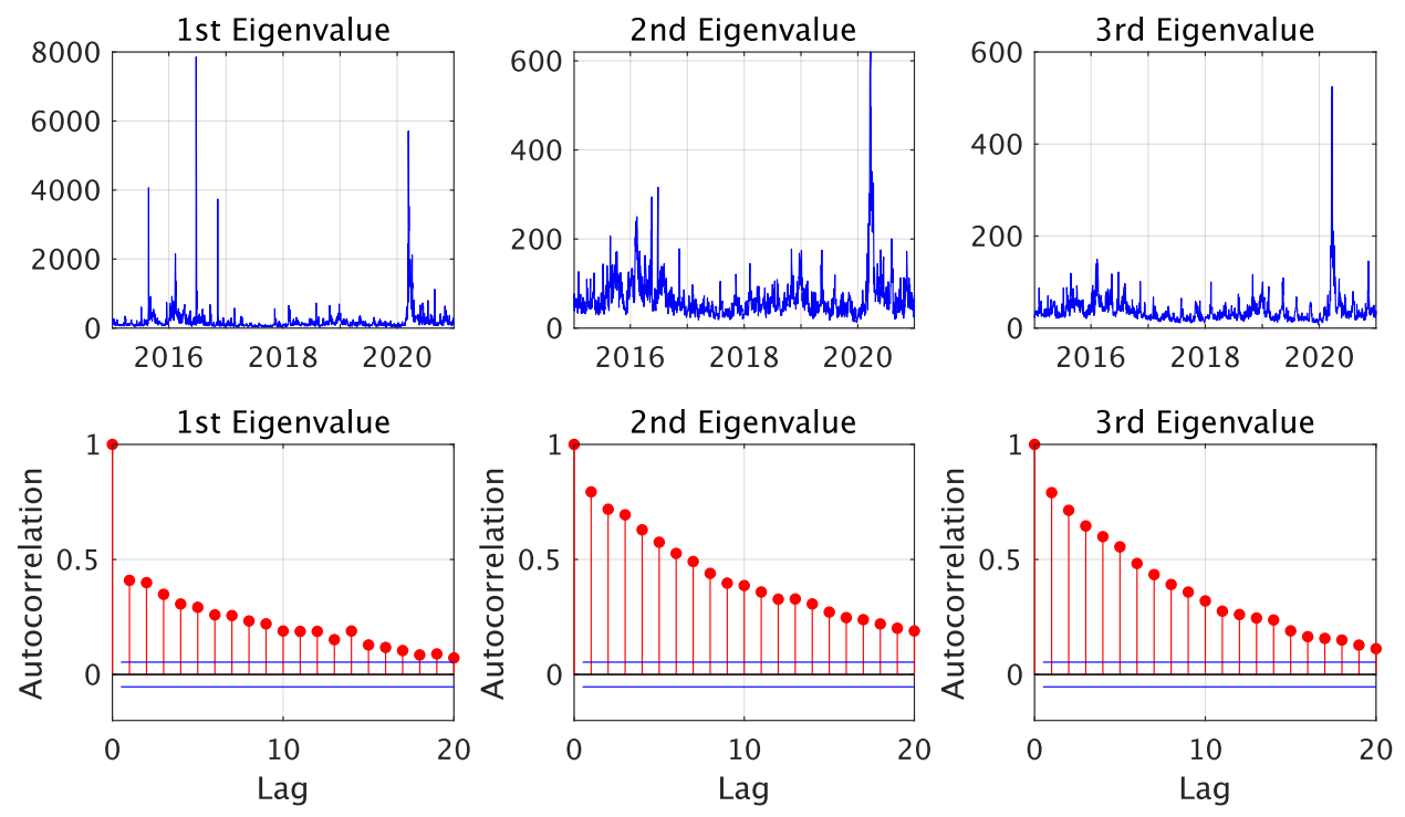
2.3. PCA for High-Frequency Data

To estimate an HDCM, we show the PCA for the realized covariance matrix estimated by high-frequency data following [29]. Here, y j , t is the j-th intraday log-return observed on day t. The realized covariance matrix is defined as follows:
Σ ^ Y t = j = 1 M y j , t y j , t .
We assume d > M ; thus, the realized covariance matrix is estimated under this assumption.

2.3.1. POET Method

The eigenvalues of the realized covariance matrix Σ ^ Y t are λ ^ 1 t > λ ^ 2 t > > λ ^ d t , and ξ ^ 1 t , ξ ^ 2 t , , ξ ^ d t denote the corresponding eigenvectors. If r ^ is the estimator of r, which is the number of factors, Σ ^ Y t has a spectral decomposition as follows:
Σ ^ Y t = j = 1 r ^ λ ^ j t ξ ^ j t ξ ^ j t + Σ ^ Z t ,
where Σ ^ Z t is the covariance matrix of the residual process, which is calculated by Σ ^ Z t = j = r ^ + 1 d λ ^ j t ξ ^ j t ξ ^ j t . Here, even if the common factor X t is an unobservable process, if Σ Z is sufficiently sparse, β Σ X t β in Equation (2) can be estimated using the eigenvalues and eigenvectors of Σ ^ Y t [24]. Therefore, we estimate the sparse residual covariance matrix, and then estimate a high-dimensional covariance matrix Σ ^ Y t S as follows:
Σ ^ Y t S = j = 1 r ^ λ ^ j t ξ ^ j t ξ ^ j t + Σ ^ Z t S ,
where Σ ^ Z t S is the estimated sparse residual covariance matrix. This high-dimensional covariance estimator consists of the POET for low-frequency data of [19] and the PCA approach adopted in [24,25] for high-frequency data.

2.3.2. Shrinkage POET Method

The PCA which is used in Equation (5) is effective, when dimension d is fixed and the sample size (the number of observations in a day) is sufficiently large. However, it is well-known that in situations where d > M , the eigenvalues and eigenvectors of the realized covariance matrix are not consistent estimators in the sense that they are quite far from the true values [16]. To deal with this problem, we use shrinkage POET (SPOET), proposed by [31], which corrects biases of empirical eigenvalues and estimates an HDCM as follows:
Σ ˜ Y t S = j = 1 r λ ˜ j t ξ ^ j t ξ ^ j t + Σ ^ Z t S ,
where λ ˜ j t = max { λ ^ j t c ¯ d / M , 0 } . In addition, as c ¯ is unknown, we have to estimate it. In this paper, we follow [31] to estimate as follows:
c ^ = ( tr ( Σ ^ Y t ) j = 1 r λ ^ j ) / ( d r d r / M ) .

3. Forecasting Models

In this section, in order to forecast an HDCM, we introduce forecasting models based on the PCA. We denote the eigenvalues as:
σ f t = [ λ 1 t , , λ r t ] .
Since these eigenvalues are the variances of factors, we can consider models similar to the time-series model of the realized variance of asset returns [29]. To model the eigenvalues, we use the exponentially weighted moving average (EWMA), (Vector) HAR, and (Vector) AR models, the same as [29]. All models except the EWMA model can be easily estimated using OLS.

3.1. EWMA Model

In this paper, we use the EWMA model developed by [33] as a benchmark model, as follows:
σ f t + 1 | t = a σ f t | t 1 + ( 1 a ) σ t ,
where a is the decaying parameter that determines the weight of the observed value 1 period before the forecast, and we set a = 0.94 following the framework of a RiskMetrics approach [33]. As this model is easy to implement to forecast volatility and covariance, a lot of studies use it in practice.

3.2. VAR Model

We introduce the AR(1) and VAR models based on high-frequency factor model as:
λ i t = a 0 , i + a 1 , i λ i t 1 + ε i t , i = 1 , , r ,
σ f t = A 0 + A 1 σ f t 1 + ε f t ,
where a k , i , A k , k = 0 , 1 are scalar parameters and parameter matrices, respectively. ε i t denotes the innovation term.
Andersen et al. [34] pointed out that the logarithmic standard deviations are closer to a normal distribution in general compared to the realized variance itself, and modeling and forecasting log volatility guarantee that the fitted and forecasted volatility are non-negative without any constrains. Therefore, we also apply the logarithmic eigenvalues to these models.

3.3. V-HAR Model

In this subsection, we introduce the HAR model and V-HAR model which are proposed by [7,35], respectively. These models are usually applied to forecasting both univariate and multivariate realized volatility. The HAR model is advantaged for approximating the long memory properties using daily, weekly and monthly volatility. Also, given the multivariate framework, the impact of the short- and long-term volatility of another asset can be included in a forecast of the volatility of one asset. To use these models, we calculate the weekly and monthly eigenvalues as follows:
λ i , W t = 1 5 j = 0 4 λ i t j ,
λ i , M t = 1 22 j = 0 21 λ i t j .
In addition, we define that σ f . W t = [ λ 1 , W t , , λ r , W t ] and σ f . M t = [ λ 1 , M t , , λ r , M t ] . We construct the HAR and V-HAR models using daily, weekly, and monthly eigenvalues as follows:
λ i t = a 0 , i + a 1 , i λ i t 1 + a 2 , i λ i , W t 1 + a 3 , i λ i , M t 1 + ε i t , i = 1 , , r ,
σ f t = A 0 + A 1 σ f t 1 + A 2 σ f , W t 1 + A 3 σ f , M t 1 + ε f t .
where a k , i , A k , k = 0 , , 3 are scalar parameters and parameter matrices, respectively. Similar to AR and VAR models, these models are transformed into logarithmic models.
Using these models, we can obtain the forecasted HDCM, S ^ t + 1 , as follows:
S ^ t + 1 = j = 1 r ^ λ ˇ j t + 1 ξ ^ j t ξ ^ j t + Σ ^ Z t S ,
where λ ˇ j t + 1 denotes the forecasted j-th eigenvalues at t + 1 , ξ ^ j is the eigenvectors corresponding to the forecasted eigenvalues, and Σ ^ Z t S is the sparse residual covariance matrix at t. Hence, in this model, we use the eigenvectors and sparse residual covariance matrix at t and the forecasted eigenvalues at t + 1 to forecast an HDCM.

4. Simulation Study

SPOET outperforms POET and the sample covariance matrix for i.i.d. data using a simulation study [31]. We now investigate the small sample performance of the POET and SPOET for a large portfolio, and show that SPOET is more accurate than POET even when applied to estimating the integrated covariance matrix in continuous Itô semi-martingale.

4.1. Simulation Design

In order to investigate the small sample performance, we performed the simulation study in a simple way according to [36,37], which treats the observed realized covariance matrix as the latent integrated covariance matrix. In this paper, we consider not the realized covariance matrix, but the high-dimensional covariance matrix estimated using (S)POET as the integrated covariance matrix. Regarding the observed realized covariance matrix, we discuss this in the Data section of the empirical analysis Section 5.1, below. Their simulation method can simulate empirically realistic sample paths of daily covariance matrices using the observed data. We use a diurnal pattern because the generated returns do not allow stochastic variation in covariances within a day. The intraday volatility pattern is modeled by means based on a diurnal U-shape function, σ d ( u ) . Therefore, we generate the intraday volatility pattern σ d ( u ) , the spot covariance matrix Σ ( u ) , and intraday asset returns as follows:
d P ( u ) = Σ ( u ) 1 / 2 d W ( u ) ,
Σ ( u ) = σ d ( u ) Σ ,
σ d ( u ) = C + A e a u + B e b ( 1 u ) ,
where we set A = 0.75 , B = 0.25 , C = 0.88929198 , and a = b = 10 , respectively, following [36,37]. In this simulation study, similar to our empirical analysis described below, we consider 202, 100, and 50 dimensional covariance matrix of 1392 days. We generate one-second prices for each day, and the realized covariance matrix is estimated by 10- and 5-min returns.

4.2. Simulation Result

We evaluate the performance of POET and SPOET by comparing the size of the estimated eigenvalues and the norm for each estimator. Table 1 and Figure 1 show the results.
First, we confirm the size of estimated eigenvalues for each estimator. The average of the first, second, and third eigenvalues of POET and SPOET for the 10- and 5-min interval realized covariance matrix are shown in Table 1. This table shows the mean, maximum and minimum values for each eigenvalue. All eigenvalues estimated by SPOET are closer to the true values than those by POET for all dimensions and all eigenvalues.
Then, we compare the estimation performance of POET and SPOET using | | S ^ S | | 2 , | | S ^ S | | F , MSE (mean square error). S ^ and S denote the estimation and the integrated covariance matrix, respectively. Our result is reported in Figure 1; the x axis shows the dimension and the interval, for example, 200 ( 10 ) means the 202 dimensional covariance estimated using 10-min interval intraday returns. Although the colors of the line show the thresholding types, we cannot see the difference between them. The biggest thing to notice is that no matter under what loss functions, interval, or dimension, SPOET always outperforms POET. Except for MSE, the errors become smaller as the return interval becomes shorter and the dimension of the covariance matrix becomes smaller. These results show that what is stated by [31], “It affirms the claim that shrinkage of spiked eigenvalues is necessary to maintain good performance when the spikes are not sufficiently large” is also true for the estimation of HDCM using price process.

5. Empirical Analysis

First, we explain the data we used and its descriptive statistics. Then, the forecasting models are evaluated by loss functions and a variance of portfolio, which is estimated by forecasted covariance matrix.

5.1. Data

We use the high-frequency data of individual stocks included in the Nikkei 225, which we bought from Nikkei NEEDS-TICK data. The sample period covers 1392 days, from 1 January 2015 to 31 December 2020. We adopt a maximum of 202 individual stocks that have traded continuously during the sample period. In addition, we consider not only 202 stocks but also 100 and 50 stocks, and, for each dimension, we estimate the realized covariance matrix using 10- and 5-min interval intraday returns. In order to estimate the realized covariance matrix, we use MFE Toolbox (https://www.kevinsheppard.com/MFE_Toolbox (accessed on 1 November 2022)), which was published by Prof. Kevin Sheppard. However, only for the realized covariance matrix of 50 stocks, we did not consider the matrix with 5-min intervals. This is because high-frequency intraday returns with 5-min intervals have 60 observations in a day, which is not appropriate to the objective of this study, i.e., the situation where the sample size is smaller than the dimension of the matrix.
Figure 2 shows the time series of first, second, and third eigenvalues estimated by POET and their autocorrelation. Similar to [29], each eigenvalue series shows a variation similar to volatility. In addition, since the autocorrelation is significant and positive, the autoregressive models, like the AR and HAR models, are effective to model the eigenvalues. The results of the estimated eigenvalues by SPOET can be observed as the same as POET; therefore, we omit them here.
Table 2 presents the size of the first, second, and third eigenvalues of the 200 dimensional realized covariance matrix estimated by POET and SPOET. We can find that when the number of factors is three, SPOET can estimate the shrinkage eigenvalues for mean, max, and min.

5.2. Out-of-Sample

We evaluate all models using the rolling-window method during the out-of-sample period. These models are reestimated everyday and set 500 days as the rolling window. The process of evaluating the forecasting performance requires using some loss functions, the Diebold–Mariano (DM) test proposed by [38] and the model confidence set (MCS) developed by [39]. Then, based on the forecasted covariance matrix, we construct a portfolio and calculate the variances of returns that are generated by each portfolio.

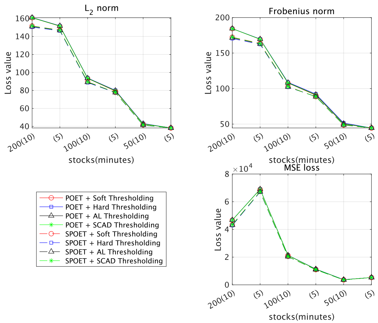
5.2.1. Loss Functions and MCS

In this paper, to evaluate the forecasting performance at time t, we use the Frobenius distance and MSE which are known to be robust in the presence of noisy covariance matrix proxies [40].
Frobenius : tr ( S ^ t Σ t ) ( S ^ t Σ t ) ,
MSE : vech ( Σ t S ^ t ) vech ( Σ t S ^ t ) ,
where S ^ t is the forecasted HDCM and Σ t denotes an integrated covariance matrix at t. As a proxy of an integrated covariance matrix, we use an HDCM based on an ex-post observed realized covariance matrix. Then, the 80 % MCS is calculated by the result of loss functions. We also calculated the 90 % and 70 % MCSs, and their results selected the same models with 80 % MCS, therefore, we describe the result of 80 % MCS. The MCS is calculated by the block bootstrap method with the length of the block beginning at two and the number of bootstrap samples being 10,000.
Table 3 and Table 4 show the number of factors for each dimension and the results of loss functions and MCS using the realized covariance matrix estimated by 10- and 5-min intraday returns. The number of factors is estimated by Equations (3) and (4). The results use the soft thresholding method for the sparse estimation of the residual covariance matrix. When other sparse estimations are used, the value of the loss changes, but the results remain the same. Additionally, the MCS is used for the results of a total of 18 models using POET and SPOET for each number of stocks.
Table 3 shows the results of the Frobenius distance of all models. First, we compare forecast values of POET and SPOET with the same time-series model using the DM test which is the statistical hypothesis testing based on the difference of the loss to compare the forecasting accuracy between the two models. Therefore, *, **, and *** in the table denote that the value is a more accurate forecast than the competitor at 10 % , 5 % , and 1 % significant levels; for example, in the 200 dimension, since the forecast value 210.41 of the AR model with SPOET has ***, it is more accurate than the forecast of the AR model with POET. In Table 3, for 200 and 100 dimensions, all forecast values of SPOET have better performance than POET for Frobenius loss. For 50 dimensions, almost all the models with SPOET are significant at 1 % and 5 % . On the other hand, for MSE, although a few models are improved, almost none of the models seem to improve. Therefore, overall, estimating an HDCM using SPOET improces the accuracy of forecasting compared to using POET. Then, we select the best models in terms of forecasting performance. The VAR (log), HAR (log), V-HAR (log) models driven by logarithmic eigenvalues are selected by MCS for all dimensions. In addition, from the perspective of MSE, the models selected by MCS are HAR, and V-HAR models of SPOET with 200 and 100 stocks, and the V-HAR model of SPOET with 50 stocks. Table 4 shows almost the same result as Table 3.
These results say that it is possible for the eigenvalues estimated by POET, in other words, the eigenvalues estimated by classical PCA, to be modeled and forecasted with biases under the high dimension. On the other hand, since the biases of the eigenvalues are corrected by SPOET, the forecasted values obtained using SPOET are more accurate than those obtained using POET. In addition, we compare the AR model with the HAR model, and the VAR model with the V-HAR model. Both the HAR model and the V-HAR model show smaller losses; hence, approximating the long memory property for eigenvalue-driven models is effective.

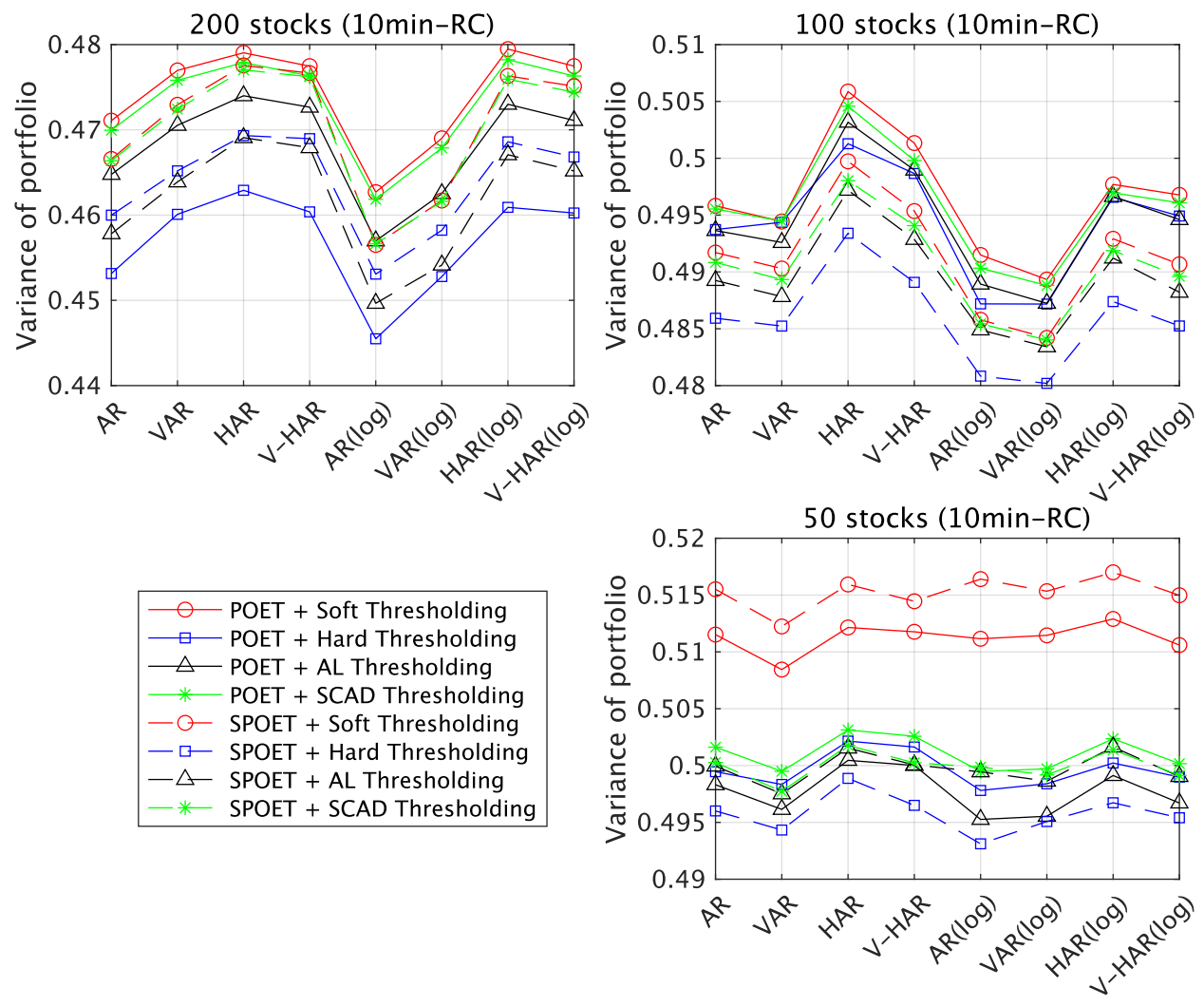
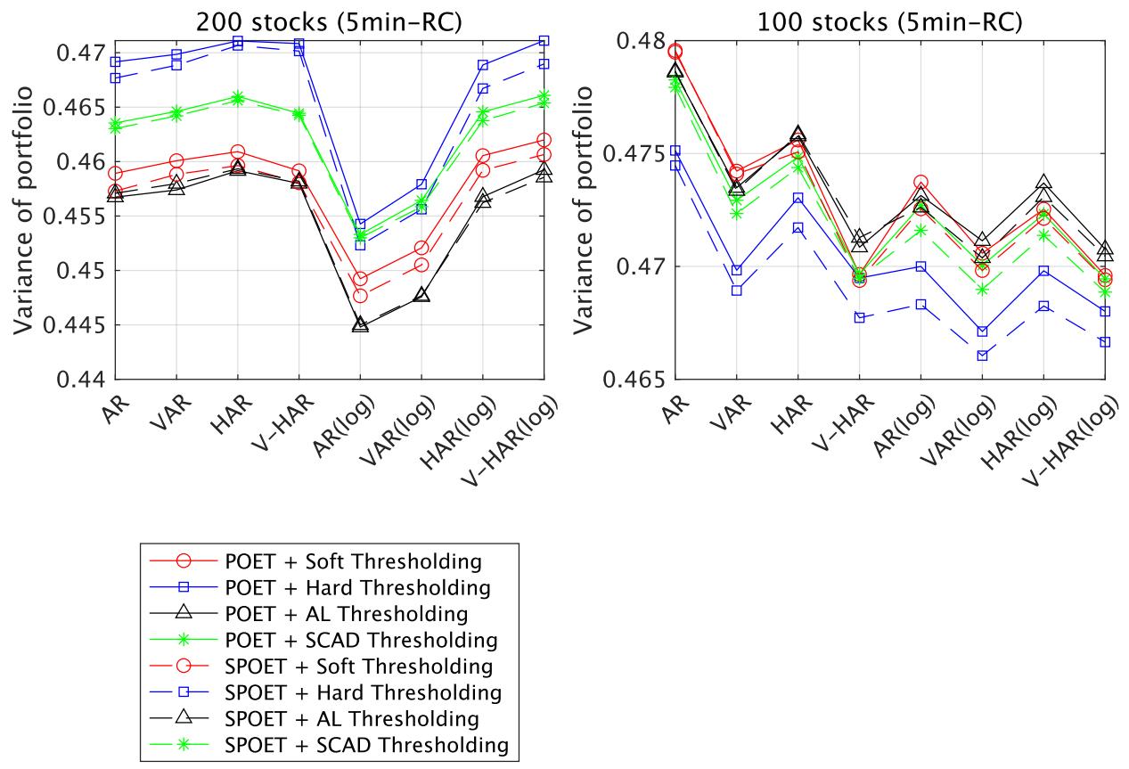
5.2.2. Portfolio Performance

In order to determine the best model among our proposed and benchmark models, we compare their forecasting performance in an economic context. In this paper, we consider that the model which generates a smaller variance portfolio than other models is better. The portfolio is estimated by the minimum variance portfolio without short selling. The weight of each stock including a portfolio can be calculated based on the results of the following optimization problem:
min ω t ω t S ^ t ω t , s . t . i = 1 N ω t , i = 1 , 0 ω t , i 1 ,
where ω t denotes the vector of portfolio weight at t, and S ^ t denotes the high-dimensional covariance matrix forecasted by each model.
Figure 3 and Figure 4 show the average portfolio variance estimated by POET, SPOET, and each forecasting model. The x axis shows the types of models and the y axis shows the portfolio variance. The color of each line denotes the thresholding method of the residual covariance matrix, the red, blue, black, and green show the soft, hard, AL, and SCAD thresholding, respectively. In addition, the results of POET are indicated by the solid lines and those for SPOET are indicated by the dotted lines.
In Figure 3, the result of 10-min realized covariance matrix is shown. For the 200 dimensions, the pair of POET and hard thresholding have the best performance among competing models. However, comparing POET and SPOET with the same sparse estimation shows that the results with SPOET generate portfolios with smaller variance except for hard thresholding. For the 100 dimensions, the pair of SPOET and hard are the best. Additionally, for all models, the forecasting models with SPOET have better performance than those with POET. Finally, for the 50 dimensions, we cannot find the differences between POET and SPOET, and the soft thresholding performs worse than other thresholding methods.
Figure 4 shows the result of a 5-min realized covariance matrix. The differences in performance between POET and SPOET become smaller than in the case of the 10-min realized covariance matrix. This is perhaps because increasing the number of intraday returns makes the classical PCA performance improve. However, for both dimensions, the performances of SPOET are still better than POET.

6. Conclusions

In this study, we constructed the HDCM forecasting models using high-dimensional PCA. In particular, the previous studies show that to estimate the latent factors, POET is used. However, it is known that when the dimension is greater than the sample size, the eigenvalues estimated by classical PCA have biases. Therefore, in order to estimate the eigenvalues more accurately, we adopted SPOET which corrects biases of empirical eigenvalues. In addition, we combined eigenvalues and time-series models to forecast eigenvalues and covariance matrix.
In the simulation study, we generated the asset returns based on the estimated HDCM as the integrated covariance matrix and it shows that SPOET is also effective for the price process. Especially, the empirical eigenvalues of SPOET were closer to the true values than those of POET.
In the empirical analysis, we constructed some forecasting models of HDCM using a number of individual stocks traded on Nikkei 225. Almost all our proposed models which use SPOET show better performance than the other models which use POET. In addition, in terms of economic performance, our models can generate a smaller variance than benchmarks in most cases. This study applied SPOET discussed under the i.i.d. setting to the continuous Itô semi-martingale setting for simulation study and empirical analysis. Thus, theoretical results are needed in the future.

Author Contributions

Conceptualization, H.S. and T.M.; software, H.S.; data curation, H.S. and T.M.; formal analysis, H.S.; writing—original draft preparation, H.S.; writing—review and editing, H.S. and T.M.; supervision, T.M. All authors have read and agreed to the published version of the manuscript.

Funding

This study is partly supported by the Institute of Statistical Mathematics (ISM) cooperative research program (2022-ISMCRP-2024), JSPS KAKENHI Grant Number 21K01433, and Grant-in-Aid for JSPS Fellows Grant Number 22J10285.

Data Availability Statement

The real data we used can be bought from Nikkei NEEDS-TICK data.

Conflicts of Interest

The authors declare that they have no conflict of interest.

References

  1. Bauwens, L.; Laurent, S.; Rombouts, J. Multivariate GARCH models: A survey. J. Appl. Econom. 2006, 21, 79–109. [Google Scholar] [CrossRef] [Green Version]
  2. Engle, R.; Kroner, K. Multivariate simultaneous generalized arch. Econom. Theory 1995, 11, 122–150. [Google Scholar] [CrossRef]
  3. Tse, Y.; Tsui, A. A multivariate generalized autoregressive conditional heteroscedasticity model with time-varying correlations. J. Bus. Econ. Stat. 2002, 20, 351–362. [Google Scholar] [CrossRef]
  4. Engle, R. Dynamic conditional correlation: A simple class of multivariate generalized autoregressive conditional heteroskedasticity models. J. Bus. Econ. Stat. 2002, 20, 339–350. [Google Scholar] [CrossRef]
  5. Barndorff-Nielsen, O.; Shephard, N. Econometric analysis of realized covariation: High frequency based covariance, regression, and correlation in financial economics. Econometrica 2004, 72, 885–925. [Google Scholar] [CrossRef]
  6. Barndorff-Nielsen, O.; Hansen, P.; Lunde, A.; Shephard, N. Multivariate realised kernels: Consistent positive semi-definite estimators of the covariation of equity prices with noise and non-synchronous trading. J. Econom. 2011, 162, 149–169. [Google Scholar] [CrossRef] [Green Version]
  7. Bubák, V.; Kočenda, E.; Žikeš, F. Volatility transmission in emerging European foreign exchange markets. J. Bank. Financ. 2011, 35, 2829–2841. [Google Scholar] [CrossRef] [Green Version]
  8. Golosnoy, V.; Gribisch, B.; Liesenfeld, R. The conditional autoregressive Wishart model for multivariate stock market volatility. J. Econom. 2012, 167, 211–223. [Google Scholar] [CrossRef] [Green Version]
  9. Bauwens, L.; Storti, G.; Violante, F. Dynamic conditional correlation models for realized covariance matrices. CORE DP 2012, 60, 104–108. [Google Scholar]
  10. Engle, R.; Ledoit, O.; Wolf, M. Large dynamic covariance matrices. J. Bus. Econ. Stat. 2019, 37, 363–375. [Google Scholar] [CrossRef] [Green Version]
  11. Nakagawa, K.; Imamura, M.; Yoshida, K. Risk-based portfolios with large dynamic covariance matrices. Int. J. Financ. Stud. 2018, 6, 52. [Google Scholar] [CrossRef]
  12. Moura, G.; Santos, A.; Ruiz, E. Comparing high-dimensional conditional covariance matrices: Implications for portfolio selection. J. Bank. Financ. 2020, 118, 105882. [Google Scholar] [CrossRef]
  13. De Nard, G.; Engle, R.; Ledoit, O.; Wolf, M. Large dynamic covariance matrices: Enhancements based on intraday data. J. Bank. Financ.. 2022, 138, 106426. [Google Scholar] [CrossRef]
  14. Trucíos, C.; Mazzeu, J.; Hallin, M.; Hotta, L.; Valls Pereira, P.L.; Zevallos, M. Forecasting conditional covariance matrices in high-dimensional time series: A general dynamic factor approach. J. Bus. Econ. Stat. 2021, 1–13. [Google Scholar] [CrossRef]
  15. Wang, Y.; Zou, J. Vast volatility matrix estimation for high-frequency financial data. Ann. Stat. 2010, 38, 943–978. [Google Scholar] [CrossRef] [Green Version]
  16. Tao, M.; Wang, Y.; Yao, Q.; Zou, J. Large volatility matrix inference via combining low-frequency and high-frequency approaches. J. Am. Stat. Assoc. 2011, 106, 1025–1040. [Google Scholar] [CrossRef]
  17. Kim, D.; Wang, Y.; Zou, J. Asymptotic theory for large volatility matrix estimation based on high-frequency financial data. Stoch. Process. Their Appl. 2016, 126, 3527–3577. [Google Scholar] [CrossRef] [Green Version]
  18. Shen, K.; Yao, J.; Li, W. Forecasting high-dimensional realized volatility matrices using a factor model. Quant. Financ. 2020, 20, 1879–1887. [Google Scholar] [CrossRef] [Green Version]
  19. Fan, J.; Liao, Y.; Mincheva, M. Large covariance estimation by thresholding principal orthogonal complements. J. R. Stat. Soc. Ser. B Stat. Methodol. 2013, 75, 603–680. [Google Scholar] [CrossRef] [Green Version]
  20. Fan, J.; Furger, A.; Xiu, D. Incorporating global industrial classification standard into portfolio allocation: A simple factor-based large covariance matrix estimator with high-frequency data. J. Bus. Econ. Stat. 2016, 34, 489–503. [Google Scholar] [CrossRef]
  21. Brownlees, C.; Nualart, E.; Sun, Y. Realized networks. J. Appl. Econom. 2018, 33, 986–1006. [Google Scholar] [CrossRef]
  22. Koike, Y. De-biased graphical lasso for high-frequency data. Entropy 2020, 22, 456. [Google Scholar] [CrossRef] [Green Version]
  23. Fan, J.; Fan, Y.; Lv, J. High dimensional covariance matrix estimation using a factor model. J. Econom. 2008, 147, 186–197. [Google Scholar] [CrossRef] [Green Version]
  24. Aït-Sahalia, Y.; Xiu, D. Using principal component analysis to estimate a high dimensional factor model with high-frequency data. J. Econom. 2017, 201, 384–399. [Google Scholar] [CrossRef]
  25. Dai, C.; Lu, K.; Xiu, D. Knowing factors or factor loadings, or neither? Evaluating estimators of large covariance matrices with noisy and asynchronous data. J. Econom. 2019, 208, 43–79. [Google Scholar] [CrossRef]
  26. Zou, H. The adaptive lasso and its oracle properties. J. Am. Stat. Assoc. 2006, 101, 1418–1429. [Google Scholar] [CrossRef] [Green Version]
  27. Fan, J.; Li, R. Variable selection via nonconcave penalized. J. Am. Stat. Assoc. 2001, 96, 1348–1360. [Google Scholar] [CrossRef]
  28. Cai, T.; Liu, W. Adaptive thresholding for sparse covariance matrix estimation. J. Am. Stat. Assoc. 2011, 106, 672–684. [Google Scholar] [CrossRef] [Green Version]
  29. Jian, Z.; Deng, P.; Zhu, Z. High-dimensional covariance forecasting based on principal component analysis of high-frequency data. Econ. Model. 2018, 75, 422–431. [Google Scholar] [CrossRef]
  30. Yata, K.; Aoshima, M. Effective PCA for high-dimension, low-sample-size data with noise reduction via geometric representations. J. Multivar. Anal. 2012, 105, 193–215. [Google Scholar] [CrossRef] [Green Version]
  31. Wang, W.; Fan, J. Asymptotics of empirical eigenstructure for high dimensional spiked covariance. Ann. Stat. 2017, 45, 1342–1374. [Google Scholar] [CrossRef] [PubMed]
  32. Rothman, A.; Levina, E.; Zhu, J. Generalized thresholding of large covariance matrices. J. Am. Stat. Assoc. 2009, 104, 177–186. [Google Scholar] [CrossRef]
  33. J.P. Morgan/Reuters. Risk Metrics. Thechnical Document, 4th ed.; J.P. Morgan/Reuters: New York, NY, USA, 1996. [Google Scholar]
  34. Andersen, T.; Bollerslev, T.; Diebold, F. Roughing it up: Including jump components in the measurement, modeling, and forecasting of return volatility. Rev. Econ. Stat. 2007, 89, 701–720. [Google Scholar] [CrossRef]
  35. Corsi, F. A simple approximate long-memory model of realized volatility. J. Financ. Econom. 2009, 7, 174–196. [Google Scholar] [CrossRef]
  36. Andersen, T.; Dobrev, D.; Schaumburg, E. Jump-robust volatility estimation using nearest neighbor truncation. J. Econom. 2012, 169, 75–93. [Google Scholar] [CrossRef] [Green Version]
  37. Bollerslev, T.; Patton, A.; Quaedvlieg, R. Modeling and forecasting (un)reliable realized covariances for more reliable financial decisions. J. Econom. 2018, 207, 71–91. [Google Scholar] [CrossRef] [Green Version]
  38. Diebold, F.; Mariano, R. Comparing predictive accuracy. J. Bus. Econ. Stat. 1995, 13, 253–265. [Google Scholar]
  39. Hansen, P.R.; Lunde, A.; Nason, J.M. The Model Confidence Set. Econometrica 2011, 79, 453–497. [Google Scholar] [CrossRef] [Green Version]
  40. Laurent, S.; Rombouts, J.; Violante, F. On loss functions and ranking forecasting performances of multivariate volatility models. J. Econom. 2013, 173, 1–10. [Google Scholar] [CrossRef]
Figure 1. Simulation results. Notes: the x axis shows the number of stocks and the time interval of realized covariance matrix.
Axioms 11 00692 g001
Figure 2. Eigenvalues estimated by POET and sample autocorrelation functions.
Axioms 11 00692 g002
Figure 3. The variance of portfolios estimated by each model using 10-min interval intraday returns.
Axioms 11 00692 g003
Figure 4. The variance of portfolios estimated by each model using 5-min interval intraday returns.
Axioms 11 00692 g004
Table 1. Simulation results of eigenvalues.
10-min 5-min
λ 1 λ 2 λ 3 λ 1 λ 2 λ 3
Stocks Mean
TRUE194.54362.64033.081194.54362.64033.081
200POET325.517109.11158.144328.368105.50756.128
SPOET313.30896.90245.935322.15899.29749.918
TRUE104.44835.65220.452104.44835.65220.452
100POET181.29463.45136.127174.27060.16835.083
SPOET175.18557.34230.018171.14657.04431.959
TRUE49.15018.69411.18049.15018.69411.180
50POET83.80731.99519.54083.24631.38918.679
SPOET81.24329.43116.97781.91630.05917.349
Max
TRUE7843.507581.130487.2027843.507581.130487.202
200POET10,095.6981050.907806.34115,710.724985.235727.615
SPOET10,059.541941.379681.52715,692.497927.323669.703
TRUE3811.211271.343192.5453811.211271.343192.545
100POET6609.435608.361299.4454421.615524.372335.179
SPOET6579.344554.550245.6344412.434506.948310.397
TRUE1662.291209.630117.8631662.291209.630117.863
50POET2477.492448.610230.0803922.754382.988169.577
SPOET2469.275420.733202.2033918.187369.209155.799
Min
TRUE29.61210.9166.30629.61210.9166.306
200POET47.26218.21113.73938.44614.41010.803
SPOET40.19814.5559.42936.11012.5818.916
TRUE13.1156.4804.31913.1156.4804.319
100POET22.37410.8558.10323.9549.9397.046
SPOET19.5958.9716.20822.7058.9726.046
TRUE6.5552.4371.9156.5552.4371.915
50POET11.4045.5723.55012.4594.6733.687
SPOET10.1444.8572.83512.0254.3013.315
Notes: This table reports the size of eigenvalues which are first three of the integrated covariance, the POET estimator, and SPOET estimator.
Table 2. The eigenvalues estimated by POET and SPOET of 200 dimensional matrix.
10-min5-min
λ 1 λ 2 λ 3 λ 1 λ 2 λ 3
Mean
POET199.6167.3837.20175.1656.3135.14
SPOET191.7859.5529.37170.0651.2130.04
Max
POET7859.83619.82524.944930.991379.47331.24
SPOET7835.62546.92452.044909.131361.80288.60
Min
POET31.5212.467.6922.7014.257.54
SPOET28.4910.135.3620.6512.245.90
Table 3. Average forecasting losses for 10-min interval intraday returns.
10 min200 Stocks100 Stocks50 Stocks
Observations30
Factors346
FrobeniusPOETSPOETPOETSPOETPOETSPOET
AR219.06210.41 ***117.65114.12 ***54.9954.47 ***
VAR202.31195.70 ***108.42105.75 ***50.7950.65 **
HAR204.99196.76 ***111.17107.84 ***52.4552.01 ***
V-HAR199.47192.11 ***108.09105.41 ***50.6750.24 ***
AR(log)192.98184.47 ***105.79102.33 ***49.6149.14 ***
VAR(log)189.82181.66 ***103.50100.30 ***48.6248.26
HAR(log)188.63180.09 ***103.2199.75 ***48.5248.06 ***
V-HAR(log)188.57179.98 ***102.8199.41 ***48.3947.96
EWMA212.02203.34 ***115.63112.10 ***54.7354.18 ***
MSE
AR5.13074.87851.46751.41560.34840.3446 *
VAR4.86924.65191.39381.35340.32730.3262
HAR4.58064.3417 *1.32321.2742 *0.32200.3185 *
V-HAR4.37794.1552**1.28341.2416 **0.30610.3028
AR(log)5.37095.18061.53931.49870.36520.3629
VAR(log)5.28695.10631.50491.47110.36290.3624
HAR(log)4.81974.61701.37231.33040.33080.3284
V-HAR(log)4.89304.6684 *1.38541.34130.33910.3368
EWMA6.03745.77671.68221.62720.40880.4034 *
Notes: The values of MSE are ×10−4. The selected models by 80% MCS is shown in bold. *, ** , and *** denote significance at 10%, 5%, and 1% levels for DM test.
Table 4. Average forecasting losses for 5-min interval intraday returns.
5 min200 Stocks100 Stocks
Observations60
Factors34
FrobeniusPOETSPOETPOETSPOET
AR170.86165.89 ***94.8093.33 ***
VAR157.61153.61 ***87.5086.38
HAR158.93154.26 ***88.9387.58 ***
V-HAR156.93152.52 ***88.0586.72 ***
AR(log)153.33148.61 ***86.4985.11
VAR(log)150.30145.84 ***84.16 **82.94
HAR(log)149.11144.33 ***84.0182.62
V-HAR(log)148.74143.98 ***83.5682.12
EWMA171.51166.62 ***95.5294.05 ***
MSE
AR3.28533.17921.02341.0062
VAR3.09183.00000.95620.9441
HAR2.97392.87480.92120.9056
V-HAR2.87362.7764 *0.89700.8818 **
AR(log)3.79113.72461.13511.1243
VAR(log)3.70553.64691.08731.0823
HAR(log)3.34253.26471.00350.9913
V-HAR(log)3.34483.26210.99460.9816
EWMA4.51554.39921.28421.2645
Notes: The values of MSE are ×10−4. The selected models by 80% MCS is shown in bold. *, ** , and *** denote significance at 10%, 5%, and 1% levels for DM test.
Publisher’s Note: MDPI stays neutral with regard to jurisdictional claims in published maps and institutional affiliations.

