Abstract
Existing methods in portfolio management deterministically produce an optimal portfolio. However, according to modern portfolio theory, there exists a trade-off between a portfolio’s expected returns and risks. Therefore, the optimal portfolio does not exist definitively, but several exist, and using only one deterministic portfolio is disadvantageous for risk management. We proposed Dirichlet Distribution Trader (DDT), an algorithm that calculates multiple optimal portfolios by taking Dirichlet Distribution as a policy. The DDT algorithm makes several optimal portfolios according to risk levels. In addition, by obtaining the pi value from the distribution and applying importance sampling to off-policy learning, the sample is used efficiently. Furthermore, the architecture of our model is scalable because the feed-forward of information between portfolio stocks occurs independently. This means that even if untrained stocks are added to the portfolio, the optimal weight can be adjusted. We also conducted three experiments. In the scalability experiment, it was shown that the DDT extended model, which is trained with only three stocks, had little difference in performance from the DDT model that learned all the stocks in the portfolio. In an experiment comparing the off-policy algorithm and the on-policy algorithm, it was shown that the off-policy algorithm had good performance regardless of the stock price trend. In an experiment comparing investment results according to risk level, it was shown that a higher return or a better Sharpe ratio could be obtained through risk control.
1. Introduction
Financial Portfolio Management (PM) is a problem of sequentially allocating and balancing a number of funds into several risky financial assets such as stocks, bonds, or cash. The goal of portfolio management is to maximize the expected return while minimizing investment risks. Traditional portfolio management has determined the weights of financial assets based on statistical indicators. Specifically, there is a well-known portfolio optimization method called modern portfolio theory (MPT) [1]. MPT allows an efficient portfolio to be computed by using the relationship between the expected return and risk, where the risk is measured by the standard deviation of returns. While MPT provides a theoretically interpretable portfolio, it has a limitation in that a number of statistical features, which can be obtained from big data, cannot be considered [1]. Furthermore, MPT highly depends on the accurate prediction of the expected return and its standard deviation [1]. To overcome such limitations, recent studies have employed deep learning-based approaches that can automatically extract meaningful features from high-dimensional big data. In particular, applying deep reinforcement learning (Deep RL) methods to solve the portfolio management problem has continuously received attention since deep RL has the ability to learn sequential decision-making based on features extracted from deep neural networks. Hence, the importance of deep RL algorithms is being emphasized since portfolio management problems can be formulated as the sequential determination of the weight of each financial asset.
In this regard, several existing off-policy and on-policy deep RL methods have been applied to PM problems [2,3]. For off-policy RL, Ref [2] applied deep Q-learning to manage the portfolio of a fixed number of assets. In general, Q learning is an off-policy approach that can reuse experiences sampled during a training phase. Hence, off-policy approaches are usually more sample efficient than on-policy methods. However, the deep Q learning method used in [2] has a clear limitation in scalability since the architecture of the Q network is fixed depending on the number of assets, and, hence, it cannot function if the number of assets is extended. In PM, scalability means that the network can infer the weight of assets that have not been used for training. If the network is not scalable for the number of assets, it is inefficient since it should be re-trained every time a new stock is added.
To alleviate this issue, [3] applied proximal policy optimization [4], which is a well-known on-policy method, and they proposed a new architecture that can handle a dynamic number of financial assets. The fact that the model has scalability gives variety in stock selection and facilitates trading strategy construction, new assets can be added to our portfolio, or existing assets can be excluded from the portfolio. While the proposed model in [3] is scalable, it has a drawback in that on-policy methods have been mainly employed to train the network. In on-policy algorithms, the samples used to update the agent cannot be reused after updating the parameter, which often hampers sample inefficiency. Hence, it is essential to develop an off-policy algorithm to improve sample efficiency.
Furthermore, the previous models often consider a deterministic policy that can decide on only one optimal portfolio vector [2,3]. However, designing a deterministic policy is not robust to a variety of situations. If the policy network is stochastic, the agent can have more than one optimal action, and we can have portfolio options according to the expected rate of return and risk. In this regard, it is inevitable to develop scalable and multi-modal methods for PM to consider a dynamic number of assets in the test phase.
Hence, we propose Dirichlet Distribution Trader (DDT), which can incorporate both sample efficiency and scalability. To increase sample efficiency, we apply the off-policy learning algorithm to train the scalable network. In particular, we use an importance sampling technique to implement the off-policy algorithm. To compute importance weights, we define a distribution over the portfolio vector. Since the valid portfolio vector consists of the simplex, the Dirichlet distribution, which is a distribution on the simplex, is employed, while previous studies only employ a deterministic policy instead of learning a policy distribution. Furthermore, learning an optimal distribution of a portfolio has a clear benefit in a test phase. By using a portfolio distribution, we can construct various trading strategies during the test time by sampling the proper portfolio from the optimal distribution. To make the model scalable for a dynamic number of assets, we employ similar network architecture to that proposed in [5], where the information of each asset flowed identically in the network. However, we do not use Recurrent Neural Network, and use MLP for a single time step state.
In the experimental part, companies were selected from the NASDAQ 100 index to find companies with sufficient trading volume. The selected stocks are divided into Up and Down trends, and we construct datasets variously according to the trend with these stocks. After such settings, we compared the proposed model with other DRL algorithms, such as DQN, PPO, and other PM methods, as benchmarks. As a result of the experiments, our proposed model outperforms the existing methods and shows a state-of-the-art performance with respect to profit. Furthermore, we also empirically show the advantages of using the Dirichlet distribution for PM. Therefore, the contributions of our proposed methods can be summarized as follows:
- We propose a model using Dirichlet distribution, which is suitable for PM and off-policy learning.
- We conduct experiments comparing on-policy and off-policy algorithms.
- We conduct experiments with various trend datasets and compare them with other algorithms. As a result, our proposed model outperforms the other algorithms and SOTA.
- The proposed model utilizes representative values of the Dirichlet distribution to allow investors to selectively adopt investment attitudes according to risk propensities such as risk-averse and risk-seeking types.
2. Related Work
For decades, researchers in the financial field have tried to replace human traders with computers [6,7,8]. In recent years, thanks to the development of machine learning [9,10], stock investment strategies using deep learning have been proposed. These learning-based methods can be categorized into supervised learning or on/off-policy RL methods. Furthermore, we classify learning-based methods under the criterion of whether they are scalable or nonscalable. We present our categorization in Table 1.

Table 1.
Categorization of learning-based portfolio management approaches.
As with the cases of natural language processing and computer vision, the financial field has benefited from progress in machine learning. For example, Ref [11] improved the traditional momentum strategy [8] using an autoencoder. Ref [12] analyzed the effectiveness of deep neural network (DNN) within the context of stock investment strategy. Ref [13] implemented long short-term memory networks (LSTM) [9] for price prediction in the financial market and showed that LSTM can outperform memory-free classification models, including DNN. However, in general, these supervised learning-based models for stock market trading strategies are trained to make price predictions. Therefore, additional layers are needed to convert prices into action. Furthermore, training supervised learning models requires binary labels for actions, which are lacking in general cases.
Apart from the supervised learning-based methods, reinforcement learning algorithms have long been attracting the attention of researchers in the financial field. In recent years, deep reinforcement learning (DRL), which combines deep learning as a function approximation for reinforcement learning, has been adopted for many sequential decision-making problems, such as controlling robotic systems [18,19], generating humanoid motions, learning how to play video games [20,21,22,23], and learning trading strategies. These DRL models can be divided into two categories, on-policy or off-policy, depending on which algorithm is used for the model. We first introduce recent advances in DRL algorithms and second introduce recent research to apply DRL to portfolio management problems. Lee et al. [18,19] proposed a novel exploration method in DRL by using the generalization of the entropy term. Cetin and Çeliktutan [20] proposed a novel action space, called a routine space, to enable agents to learn effective behavior. Wang et al. [21] extended the classical value iteration method to multi-step RL by proposing a new multi-step Bellman optimality equation, which uses the latent space of multi-step bootstrapping. Kong et al. [22] proposed a new sampling strategy for off-policy RL, which imposes a high sampling probability to recently added data in the replay buffer to mitigate unbalanced exploitation issues between initial data and new data. Vijayan and A. [23] introduced a policy gradient algorithm that employs importance sampling for policy evaluation with a smoothed functional-based gradient estimation. Then, recent research in PM has applied DRL methods to the problem of decision-making on portfolio vectors. On-policy RL algorithms have the target policy as the policy used to make decisions in the stock market. Specifically, models for PM using on-policy RL algorithms mainly use proximal policy optimization (PPO) [4], policy gradient (PG) [24], and A2C algorithms [25]. For example, Ref [14] transplanted modern portfolio theory [26] into an RL framework to make direct mapping between market situation and trade position. In this process, Ref [14] used the on-policy RL algorithms PG and A2C compared to DQN.
On the other hand, the off-policy RL algorithms, whose target policy is different from the behavior policy, have an advantage in sample efficiency. In particular, Deep deterministic policy gradient(DDPG) [27] and deep Q-network(DQN) [28] have been widely adopted as the off-policy RL algorithms for stock market trading. For instance, Ref [16] used DQN with a convolutional neural network(CNN) to take the stock market images as input for making investment strategies. Ref [2] introduced a novel mapping function that can handle infeasible action caused by combinatorial operating spaces and applied DQN to derive PM investment strategies. Ref [17] showed model using DRL can outperform the classical RL algorithm SARSA [29] on stock market trading, and MLP has a better performance than gated recurrent unit(GRU) and CNN on feature extracting the stock market data.
However, both the on-policy and off-policy DRL models mentioned so far did not consider the scalability of the model. Although scalability is needed to handle portfolios of various sizes, only a few studies have considered the scalability of the trading model. For example, Ref [5] introduced a novel DRL structure, which consists of an ensemble of identical independent evaluators (EIIE) topology and portfolio-vector memory (PVM). By using the EIIE, including three networks CNN, RNN, and LSTM, the model is able to deal with multi-channel input, and the portfolio, with scalability. Ref [15] also used IIE to handle portfolios of various sizes. However, this model exploited the softmax function to normalize the output. Similarly, Ref [3] employed IIE for scalability, but its activation function is a Min-Max normalized function. Since both softmax and Min-Max activation functions induce one optimal portfolio vector, the existing models with scalability have a weakness in the diversity of the trading environment. On the contrary, we set the model to learn the distribution of the portfolio, making our model have robustness in a variation of the stock market.
3. Preliminaries
3.1. Financial Portfolio Management
Financial portfolio management is the task of sequentially re-balancing all weights of financial assets by considering future profits. To develop an automatic portfolio management system, in this section, we mathematically formulate the portfolio management problem.
We first define a time step t. The time step t is defined as a time slot from the opening to the closing of a stock market in which a stock can be bought or sold. At time step t, the environment (or the market) provides the agent (or the trading system) with stock data for the portfolio assets from the previous business day. Then, the time step t is divided into two periods: the period before re-balancing the portfolio and the period after re-balancing the portfolio. If our trading agent determines the portfolio based on previous stock data, it makes changes in the portfolio and its value within the time step t. Hence, we can separate the time step t into the period before the agent’s action and the term after the agent’s action.
At every time step t, an agent determines the portfolio weights based on previous stock data. The portfolio weights can be expressed as a vector of all holding weights of K assets, including both cash and non-cash assets. We denote the portfolio vector as at the period before the agent’s action in time step t.
where indicates the percentage of the ith asset among total funds. The ith entry of is denoted as , which means the weight of the ith asset before taking action. Specifically, the first element of portfolio vector, , is a proportion of cash. Then, the portfolio vector changed after taking action at time step t is denoted as . Finally, the portfolio vector at the initial time step is , which consists of cash only.
The goal of the trading agent is to determine the best based on the previous stock market data, which is encoded as a stock feature vector. The stock feature vector of the ith asset at time t is defined as
where the five features , and v represent open, high, low, close price, and volume, respectively. Then, stock feature matrix is defined by stacking for all assets as follows,
where the shape of is .
To compute the profit of , we employ the concept of the portfolio value, which is an amount of investment evaluated by reflecting the changed stock price and transaction cost. and are denoted as the portfolio value of and , respectively. To calculate a portfolio value and a changed portfolio by price fluctuations for every time step, the closing price vector at t is defined as Equation (5).
In a continuous time sequence from t to , two factors affect the portfolio value: cost and closing price fluctuations. In time step t, the agent predicts the desired portfolio . In order to change the current portfolio to the desired one, the transaction cost must be paid, which can be computed as follows,
where represents a trading amount of ith asset, and c indicates a commission rate.
After executing transactions, we can compute the pseudo portfolio weight as follows,
where and represent a set of indices of assets to sell and buy, respectively. Then, is determined by normalizing the pseudo portfolio as follows, . Furthermore, can be obtained by substituting the transaction cost, i.e., .
After computing and , we reflect on the effect of the closing price change to computing the portfolio vector at time step . When the time step changes from t to , all assets’ prices in the portfolio may be changed depending on closing price fluctuation. Hence, the portfolio value is changed. Equation (8) shows the changing formula of to , and Equation (9) shows the changing formula of to where means a price change rate vector from t to and ,
where ⊙ indicates an element-wise multiplication. The flow chart of the portfolio and portfolio value changes is shown in Figure 1.
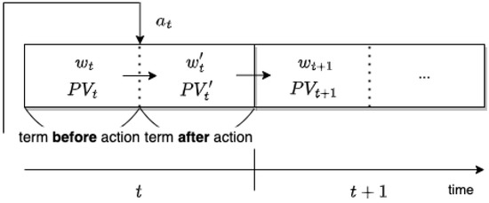
Figure 1.
Illustration of the procedure of transactions during time step t. indicates an action of the trading agent where changes to after .
3.2. Markov Decision Processes for Portfolio Management
We cast the portfolio management problem into the problem of learning an optimal strategy for sequential decision-making by using reinforcement learning algorithms. A reinforcement learning is generally formulated as a Markov decision process (MDP), which consists of a tuple where is a set of states, is a set of actions, P indicates a transition probability of a next state given state and action pair, r is a reward function mapping from to , and is a discount factor.
In the portfolio management problem, similar to [5], a state at t is defined by the stock feature matrix and the portfolio vector at the end of t as follows,
Then, an action at t is defined as a gap between the current portfolio and the desired portfolio . Therefore, the ith entry of is defined as Equation (11).
means the weight to be traded. Note that, for , and hold. If is a negative number, the ith asset must be sold, and if is a positive number, the ith asset must be bought. However, in this way, the agent cannot have a hold position except when is 0, which can lead to a large transaction cost due to frequent transactions. In this regard, we introduced a hyperparameter for threshold and truncated the action value to zero if hold to make ith asset not be traded. Further, when the agent cannot sell or buy the asset by a proportion of , is mapped to the maximum share that can be sold or bought.
For a reward function, since our agent re-invests the profits, we use a continuous compounding rate of return as a reward function, which is defined as
3.3. Distribution of a Portfolio
In this section, we define a distribution of a portfolio. Portfolio vector has innate sum-to-one constraints. In other words, a set of valid portfolio vectors is equivalent to an -dimensional simplex. Hence, to assign a distribution of a portfolio, we employ the Dirichlet distribution, which is a well-known parametric distribution over a simplex. Dirichlet distributions with concentration parameters , , … have a multivariate probability density function as follows,
where is the beta function defined as,
Note that random vector X sampled from Dirichlet distribution is an element in the simplex. Hence, and hold. This property is suitable for representing a portfolio vector. By using a Dirichlet distribution, we can define a stochastic policy over action space. We would like to emphasize that this paper is the first to employ the Dirichlet distribution to represent a stochastic policy over a portfolio vector.
4. Proposed Method
We propose a novel off-policy reinforcement learning method for scalable portfolio management by using importance sampling with the Dirichlet policy. First, to obtain scalability, we employ an architecture that can easily add new assets to a test phase. Second, to increase the sample efficiency, we also apply the importance sampling method to the Dirichlet policy that can reuse the previously sampled experience.
4.1. Architecture
We propose a scalable architecture that allows a trained policy and value network to be applied to unseen financial assets, which are not experienced during a training phase but in a test phase. The overview of the proposed network architecture is given in Figure 2. Our architecture consists of two parts: a policy network as an actor with a score net and a value network as a critic with a score net and header.
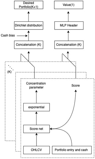
Figure 2.
Architecture of score, policy, and value networks.
First, we introduce a score network whose output is the potential goodness of each asset where is the parameter of the network. Assume that we consider K assets in our portfolio. Then, in state , we have K number of stock vectors and K number of portfolio weights . For each asset, and are an input of the score network and indicates the score of the ith asset. For all assets, the scores are predicted by the score network.
Based on , the Dirichlet policy can be defined. Since the characteristics of the Dirichlet distribution are fully determined by the concentration parameters; we define the concentration parameters as a function of scores. Specifically, since the concentration parameters must be positive, all parameters are computed as the exponential of the scores. Finally, to consider a cash asset, we add a cash bias. Hence, the distribution policy is defined as
where 1 indicates a cash bias and D indicates the desired portfolio. By using this policy, the agent can sample various portfolio vectors from the Dirichlet distribution.
Second, the value network, which is parameterized by , is defined by combining both the score network and multi-layer perceptron (MLP) header to estimate the state value, which is defined as
The state value indicates the sum of future rewards. The MLP header uses the scores of each asset as an input, and its output predicts the state value of the given policy . The detailed optimization method for updating to predict will be proposed in the next section.
By using this architecture, we can easily add or remove assets from the portfolio in a test phase. In the test phase, a new asset can be considered by estimating its score and the Dirichlet distribution can be defined over scores, including a new one. To estimate the score of a new asset, we only need for a new asset, i.e., , where can be set to zero for the first estimation. Then, a new asset can be considered by sampling a portfolio weight from a Dirichlet distribution defined over . Similarly, removing the existing asset can be achieved by defining a Dirichlet distribution defined over .
4.2. Off-Policy Optimization
In this section, we introduce the optimization technique for value header and score network . To increase sample efficiency, we propose the off-policy optimization method. First, after executing actions, the transition pairs are stored in a replay buffer where is stored to compute the importance weight. For the value header, is updated every time step with importance-weighted TD-target by using importance sampling,
where is a parameter for the target network, and B indicates the set of batch indices. For each update, we sample a batch of N transitions from the replay buffer. In Equation (18), we estimate the expectation of the squared TD loss with respect to ; however, the transition samples are generated by the previous policy , which is different from distribution . Hence, this discrepancy can be compensated by multiplying the importance weight.
To update score network , we employ the clipped ratio loss proposed in PPO [4].
where , is a clip threshold of importance ratio, and . All processes of the off-policy optimization of value function and policy is summarized in Algorithm 1.
| Algorithm 1 Drichlet Distribution Trader: DDT. |
|
4.3. Sampling by Risk
Modeling a policy of a portfolio vector by using a Dirichlet distribution has the advantage of learning multiple optimal strategies. While a deterministic policy only suggests a single optimal portfolio weight [5,15], the proposed method can model a distribution over a portfolio. Hence, our method can propose multiple sets of optimal portfolio weights. Knowing multiple optimal strategies is essential to suggesting a proper portfolio to various types of investors depending on an investment propensity, from an aggressive one to a passive one. For example, a risk-averse investor prefers a low-risk portfolio even if its expected return is low, and, on the contrary, a risk-taking one rather prefers a high-expected return even if its failure probability (or its variance) is high. In this regard, multiple portfolios are needed. Fortunately, since our policy is modeled as a distribution, we can sample multiple portfolios from the optimized distribution, and the sampled portfolios have a near-optimal expected return. By using these samples, a risk-averse or risk-taking investment can be conducted.
We propose a portfolio generation method from the resulting policy optimized by reinforcement learning. The first method uses a mean desired portfolio, which is a mean of a Dirichlet distribution, computed as follows,
where indicates the desired weight of the ith asset, and is a concentration parameter of a Dirichlet distribution defined in (16). The second method employs a mode of a Dirichlet distribution, where the desired portfolio can be computed as
The final method employs a rejection sampling based on the risk measure proposed in [1]. In this method, first, several portfolios are sampled from . Let us denote the set of N samples as where is the jth sampled portfolio vector, and N is set to be 1000 in our experiments. After sampling , second, we compute the transaction cost of each sampled portfolio and select the lowest-cost portfolios, which are denoted as where is set to be 10. Then, in the final step, we compute the risk of each portfolio as follows,
where denotes the covariance matrix of daily profit loss. By computing the risk, we can finally select three types of portfolios, which are with the highest risk, the median risk, and the lowest risk. We denote the portfolio with the lowest risk as , with the median risk as , and with the highest risk as . In the test phase, we compare these portfolio generation techniques and show the characteristics of each portfolio generation. The overview of the process of our proposed methodology, Dirichlet Distribution Trader (DDT), is given in Figure 3.
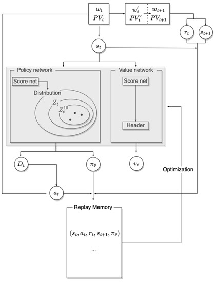
Figure 3.
Process of the Dirichlet distribution trader (DDT).
5. Experiment
5.1. Performance Metrics
The performance of trading methods is measured by the degree of return or risk. Hence, we use four metrics for evaluating the performance. The first metric is the cumulative return (CR).
where T is the entire trading period. The CR is the rate of change between the initial portfolio value and the portfolio value after an action in the terminal time step. The second metric is the average return (AR) defined as
The AR is the mean of the daily rate of change between the portfolio value at and the portfolio value at k. The third metric is the Sharpe ratio (SR),
where is a daily rate of return by desired portfolio D, is a return of risk-free asset f for benchmarking, and is the standard deviation of . The SR measures the performance or risk of an investment method compared to a risk-free asset, such as a bond. The last metric is the Maximum Drawdown (MDD) as follows,
where Min() denotes the trough portfolio value, and Max() denotes the peak portfolio value, where m is an index corresponding to the trough value. Therefore, the MDD measures the greatest fluctuation range from the highest portfolio value point to the lowest portfolio value point before a new peak is achieved, which we can consider the worst case in our investment.
5.2. Data Configuration
To use companies with sufficient trading volume and fluctuations, we selected seven companies for an experiment from among companies in the Nasdaq 100 index. As shown in Table 2, we constructed seven datasets by adding or removing stocks for a variety of experiments.
Table 2.
Datasets. HA (Hawaiian Holdings), WBA (Walgreens Boots Alliance), INCY (Incyte), BIDU (Baidu), TCOM (Trip.com), AAPL (Apple), and COST (Costco). Companies marked in bold are not included in the base dataset, Dataset 1.
Dataset 1 is the base dataset. Dataset 1 consists of stocks that include both an up-trend and a down-trend section. The down-trend dataset is a dataset in which stocks include a falling interval within the test period, such as datasets 2 and 3. Likewise, the Up-trend dataset is a dataset in which stock include a rising interval within the test period, such as dataset 4 and 5. The mix-trend dataset is a dataset that mixes the Up-trend dataset and the Down-trend dataset, which are datasets 6 and 7. All datasets are divided into two periods, one for training and one for testing in Table 3, and the closing price plots of the seven stocks during the full period are shown in Figure 4.
Table 3.
Train and test period.
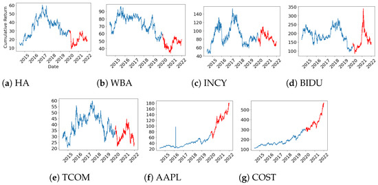
Figure 4.
Closing price of the seven stocks in the experiments: Before January 2020, the closing price plot during the training period is shown, and after that, the closing price during the test period is shown.
5.3. Scalability Experiment
5.3.1. Experiment Setup
To test the scalability of the proposed model, we compare DDT-B, a model trained on dataset 1 only, with other nonscalable models, including DDT-A, in all datasets. If we run the experiment on dataset n , the nonscalable models are trained during the training period of dataset n and tested in the test period of dataset n, but the scalable model DDT-B is trained only during the training period of dataset 1 and tested in the test period of dataset n. Whereas if , DDT-A equals DDT-B. Therefore, even if a new stock is added, DDT-B infers independently between the stocks. These are shown in Table 4.
Table 4.
Combinations of datasets used for the scalability experiment.
We used DDPG [27], DQN [28] as Deep RL baselines and EW (Equal Weight) as a traditional baseline in this experiment. Therefore, we confirmed the scalability of our model by comparing the performance difference between these baselines and DDT-A, which was trained with data from all stocks in the portfolio, and DDT-B, which was not trained with data on new stocks.
5.3.2. Experiment Results
The results of this experiment are shown in Table 5. As shown in Figure 5, except for dataset 7, our model, DDT-A, obtained the highest CR compared to other baseline algorithms. When DDT-B and DDT-A are compared, DDT-B’s CR is almost the same as DDT-A’s CR, and dataset 4 showed the largest difference of . Therefore, DDT-B is scalable as it has almost the same cumulative return as DDT-A, which has been trained with all stocks.
Table 5.
Test results of the scalability experiment. The best results are marked as bold font.

Figure 5.
Cumulative returns for the seven datasets of algorithms for the scalability test.
In the AR results, except for datasets 5 and 7, DDT-A obtained the highest AR, and in datasets 5 and 7, EW obtained the highest AR. In the results of SR, DDT-A achieved the highest SR in all datasets. It means that our model produces good returns against the risk of stock price volatility. In the results of MDD, except for dataset 5, DQN obtained the best results. This is because the action of DQN is discrete, so it acted conservatively during the maximum fall period.
5.4. On-Policy and Off-Policy Experiment
5.4.1. Experiment Setup
We used DDT-A as the off-policy algorithm, PPO as the on-policy algorithm, and DDT-On, which was a trained DDT with an on-policy algorithm. In this experiment, we compare the results of the on-policy algorithm that uses samples more inefficiently than the off-policy algorithm in each dataset with different trends by comparing the off-policy algorithm and the on-policy algorithm. All algorithms used for this experiment are summarized in Table 6.
Table 6.
Test results of On-Off experiment. The best results are marked as bold font.
5.4.2. Experiment Results
The results of this experiment are shown in Table 6. As shown in Figure 6, in the results of CR, DDT-A obtained the highest CR in all datasets. In particular, in datasets 1, 2, and 3, which are datasets that do not include AAPL or COST, where stock prices increase monotonically, the on-policy algorithms obtained lower CR, SR, and AR than DQN and DDPG, which are the off-policy algorithms of the previous experiment. In the results of SR, Except for datasets 4 and 7, DDT-A obtained the best SR, and in datasets 4 and 7, PPO obtained the best SR with a slight difference from DDT-A. In the results of AR, DDT-A obtained the best AR in all datasets, and in the results of MDD, PPO obtained the best MDD in all datasets. As a result, if stocks with the same trend in both the train and test data are not included in the portfolio, the performance difference between the on-policy algorithm and the off-policy is wider than in the case where it is not.

Figure 6.
Cumulative returns for the seven datasets of algorithms for the On-Off test.
5.5. Risk-Aware Portfolio Management Experiment
5.5.1. Experiment Setup
We use three samples of DDT-A whose risk level is High, Mid, and Low, calculated according to Equation (22) and these are denoted by , , and in Section 4.3. These three samples are determined from among the ten low-cost samples of any ten thousand samples of the Dirichlet distribution. During the test period, an action is created by selecting only one sample of the same risk level among these three samples.
5.5.2. Experiment Results
The results of this experiment are shown in Table 7. In dataset 1, high-risk trading obtained the highest CR and AR, but low-risk trading obtained the best values for SR and MDD. In datasets 2 and 3, which are down-trend datasets, low-risk trading obtained the highest CR and AR. For SR, mid-risk trading and low-risk trading obtained the best values, respectively. However, looking at Figure 7, low-risk trading reached a high peak near 100%, but it formed a large drawdown after that, and mid-risk trading obtained the best MDD. In datasets 4 and 5, which are up-trend datasets, high-risk trading obtained the highest CR and AR. For SR, mid-risk trading obtained the best results, and for MDD, low-risk trading got the best results. In dataset 6, mid-risk trading achieved the best results in all metrics, in dataset 7, low-risk trading obtained the best results in all metrics.
Table 7.
Test results of the sampling-by-risk experiment. The best results are marked as bold font.
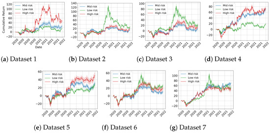
Figure 7.
Cumulative returns for the seven datasets of algorithms for the sampling test.
Specifically, in MDD, except for dataset 6, the low-risk or mid-risk result is better than the MDD of PPO in the previous experiment, and the best MDD of dataset 6, −25.899 of low risk, is also not much different from the −25.424 of PPO.
This experiment shows the characteristics of trading according to risk level. In general, high-risk investments expect high returns. These expectations are met in the up-trend dataset but not in the down-trend dataset. Further, in the downtrend dataset, low-risk has a SR similar to or much higher than that of mid-risk. On the other hand, mid-risk has better MDD than low-risk. Therefore, if SR is the most important criterion, low-risk investment can be considered, and if MDD is the most important criterion, mid-risk investment can be considered.
That is, we have the advantage of being able to select samples that reflect these characteristics according to the level of risk.
6. Conclusions
We proposed a Dirichlet Distribution Trader (DDT) that is a scalable DRL model for selectively managing portfolios according to risk. Its policy has a Dirichlet sistribution in order for an agent to generate multiple portfolio samples. Therefore, our algorithm can selectively manage the portfolio according to the level of risk after selecting 10 portfolios with low transaction costs. In the Risk-Aware Portfolio Management Experiment, we showed that the cumulative returns of portfolios corresponding to each of the three risk levels had distinct characteristics according to the trend of the dataset and showed the need for selective portfolio management. In addition, since the value can be obtained from the distribution, efficient training is possible through off-policy learning by importance sampling, and we showed in the on-policy and off-policy experiment that it has better performance than on-policy learning. Our model is not limited to the number of portfolio stocks and has the scalability to adjust the weight of new stocks added to the portfolio even if only three stocks in the base dataset are learned. Furthermore, in the scalability experiment, DDT-A, which is trained on only three stocks, showed almost the same performance as DDT-B, which is trained for all stocks in the portfolio. Based on these advantages, comparative experiments show that DDT is superior to other algorithms in risk metrics and return metrics.
Author Contributions
Conceptualization, H.Y. and K.L.; methodology, H.Y.; software, H.Y.; validation, H.Y., H.P. and K.L.; formal analysis, H.Y. and K.L.; investigation, H.Y.; resources, H.Y.; data curation, H.Y.; writing—original draft preparation, K.L.; writing—review and editing, H.P.; visualization, H.Y.; supervision, K.L.; project administration, K.L.; funding acquisition, K.L. All authors have read and agreed to the published version of the manuscript.
Funding
This research was funded by the IITP grant funded by the Korea government (MSIT) (No. 2021-0-01341, AI Graduate School Program, CAU).
Institutional Review Board Statement
Not applicable.
Informed Consent Statement
Not applicable.
Data Availability Statement
Not applicable.
Conflicts of Interest
The funders had no role in the design of the study; in the collection, analyses, or interpretation of data; in the writing of the manuscript; or in the decision to publish the results.
Abbreviations
The following abbreviations are used in this manuscript:
| IITP | Institute for Information and Communications Technology Promotion |
| MSIT | Ministry of Science and ICT |
References
- Markowitz, H. Portfolio Selection. J. Financ. 1952, 7, 77–91. [Google Scholar] [CrossRef]
- Park, H.; Sim, M.K.; Choi, D.G. An intelligent financial portfolio trading strategy using deep Q-learning. Expert Syst. Appl. 2020, 158, 113573. [Google Scholar] [CrossRef]
- Betancourt, C.; Chen, W.H. Deep reinforcement learning for portfolio management of markets with a dynamic number of assets. Expert Syst. Appl. 2021, 164, 114002. [Google Scholar] [CrossRef]
- Schulman, J.; Wolski, F.; Dhariwal, P.; Radford, A.; Klimov, O. Proximal Policy Optimization Algorithms. arXiv 2017, arXiv:1707.06347v2. [Google Scholar]
- Jiang, Z.; Xu, D.; Liang, J. A Deep Reinforcement Learning Framework for the Financial Portfolio Management Problem. arXiv 2017, arXiv:1706.10059. [Google Scholar]
- Grinblatt, M.; Titman, S.; Wermers, R. Momentum Investment Strategies, Portfolio Performance, and Herding: A Study of Mutual Fund Behavior. Am. Econ. Rev. 1995, 85, 1088–1105. [Google Scholar]
- Malkiel, B.G. Efficient Market Hypothesis. In Finance; Eatwell, J., Milgate, M., Newman, P., Eds.; Palgrave Macmillan UK: London, UK, 1989; pp. 127–134. [Google Scholar] [CrossRef]
- Jegadeesh, N.; Titman, S. Returns to Buying Winners and Selling Losers: Implications for Stock Market Efficiency. J. Financ. 1993, 48, 65–91. [Google Scholar] [CrossRef]
- Hochreiter, S.; Schmidhuber, J. Long Short-Term Memory. Neural Comput. 1997, 9, 1735–1780. [Google Scholar] [CrossRef]
- Krizhevsky, A.; Sutskever, I.; Hinton, G.E. ImageNet Classification with Deep Convolutional Neural Networks. Commun. ACM 2017, 60, 84–90. [Google Scholar] [CrossRef]
- Takeuchi, L.; Lee, Y.Y.A. Applying Deep Learning to Enhance Momentum Trading Strategies in Stocks; Technical Report; Stanford University: Stanford, CA, USA, 2013. [Google Scholar]
- Krauss, C.; Do, X.A.; Huck, N. Deep neural networks, gradient-boosted trees, random forests: Statistical arbitrage on the S&P 500. Eur. J. Oper. Res. 2017, 259, 689–702. [Google Scholar] [CrossRef]
- Fischer, T.; Krauss, C. Deep learning with long short-term memory networks for financial market predictions. Eur. J. Oper. Res. 2018, 270, 654–669. [Google Scholar] [CrossRef]
- Zhang, Z.; Zohren, S.; Stephen, R. Deep Reinforcement Learning for Trading. J. Financ. Data Sci. 2020, 2, 25–40. [Google Scholar] [CrossRef]
- Liang, Z.; Chen, H.; Zhu, J.; Jiang, K.; Li, Y. Adversarial Deep Reinforcement Learning in Portfolio Management. arXiv 2018, arXiv:1808.09940. [Google Scholar]
- Lee, J.; Kim, R.; Koh, Y.; Kang, J. Global Stock Market Prediction Based on Stock Chart Images Using Deep Q-Network. IEEE Access 2019, 7, 167260–167277. [Google Scholar] [CrossRef]
- Taghian, M.; Asadi, A.; Safabakhsh, R. Learning financial asset-specific trading rules via deep reinforcement learning. Expert Syst. Appl. 2022, 195, 116523. [Google Scholar] [CrossRef]
- Lee, K.; Choi, S.; Oh, S. Sparse Markov Decision Processes With Causal Sparse Tsallis Entropy Regularization for Reinforcement Learning. IEEE Robotics Autom. Lett. 2018, 3, 1466–1473. [Google Scholar] [CrossRef]
- Lee, K.; Kim, S.; Lim, S.; Choi, S.; Hong, M.; Kim, J.I.; Park, Y.; Oh, S. Generalized Tsallis Entropy Reinforcement Learning and Its Application to Soft Mobile Robots. In Proceedings of the Robotics: Science and Systems XVI, Virtual Event/Corvalis, OR, USA, 12–16 July 2020. [Google Scholar]
- Cetin, E.; Çeliktutan, O. Learning Routines for Effective Off-Policy Reinforcement Learning. In Proceedings of the 38th International Conference on Machine Learning, ICML 2021, Virtual, 18–24 July 2021; Volume 139, pp. 1384–1394. [Google Scholar]
- Wang, Y.; He, P.; Tan, X. Greedy Multi-step Off-Policy Reinforcement Learning. arXiv 2021, arXiv:2102.11717. [Google Scholar]
- Kong, S.; Nahrendra, I.M.A.; Paek, D. Enhanced Off-Policy Reinforcement Learning With Focused Experience Replay. IEEE Access 2021, 9, 93152–93164. [Google Scholar] [CrossRef]
- Vijayan, N.; Prashanth, L.A. Smoothed functional-based gradient algorithms for off-policy reinforcement learning: A non-asymptotic viewpoint. Syst. Control. Lett. 2021, 155, 104988. [Google Scholar] [CrossRef]
- Williams, R.J. Simple statistical gradient-following algorithms for connectionist reinforcement learning. Mach. Learn. 1992, 8, 229–256. [Google Scholar] [CrossRef]
- Mnih, V.; Badia, A.P.; Mirza, M.; Graves, A.; Lillicrap, T.P.; Harley, T.; Silver, D.; Kavukcuoglu, K. Asynchronous Methods for Deep Reinforcement Learning. arXiv 2016, arXiv:1602.01783. [Google Scholar]
- Ingersoll, J.; Ingersoll, J. Theory of Financial Decision Making; G-Reference, Information and Interdisciplinary Subjects Series; Rowman & Littlefield: Totowa, NJ, USA, 1987. [Google Scholar]
- Lillicrap, T.P.; Hunt, J.J.; Pritzel, A.; Heess, N.; Erez, T.; Tassa, Y.; Silver, D.; Wierstra, D. Continuous control with deep reinforcement learning. arXiv 2015, arXiv:1509.02971. [Google Scholar]
- Mnih, V.; Kavukcuoglu, K.; Silver, D.; Rusu, A.A.; Veness, J.; Bellemare, M.G.; Graves, A.; Riedmiller, M.; Fidjeland, A.K.; Ostrovski, G.; et al. Human-level control through deep reinforcement learning. Nature 2015, 518, 529–533. [Google Scholar] [CrossRef]
- Rummery, G.A.; Niranjan, M. On-Line Q-Learning Using Connectionist Systems; Technical Report; Cambridge University Engineering Department: Cambridge, UK, 1994. [Google Scholar]
Publisher’s Note: MDPI stays neutral with regard to jurisdictional claims in published maps and institutional affiliations. |
© 2022 by the authors. Licensee MDPI, Basel, Switzerland. This article is an open access article distributed under the terms and conditions of the Creative Commons Attribution (CC BY) license (https://creativecommons.org/licenses/by/4.0/).