Abstract
Proposed in this study is a modified model for a single-valued neutrosophic hesitant fuzzy time series forecasting of the time series data. The research aims at improving the previously presented single-valued neutrosophic hesitant fuzzy time series (SVNHFTS) model by including several degrees of hesitancy to increase forecasting accuracy. The Gaussian fuzzy number (GFN) and the bell-shaped fuzzy number (BSFN) were used to incorporate the degree of hesitancy. The cosine measure and the single-valued neutrosophic hesitant fuzzy weighted geometric (SVNHFWG) operator were applied to analyze the possibilities and pick the best one based on the neutrosophic value. Two data sets consist of the short and low-frequency time series data of student enrollment and the long and high-frequency data of ten major cryptocurrencies. The empirical result demonstrated that the proposed model provides higher efficiency and accuracy in forecasting the daily closing prices of ten major cryptocurrencies compared to the S-ANFIS, ARIMA, and LSTM methods and also outperforms other FTS methods in predicting the benchmark student enrollment dataset of the University of Alabama in terms of computation time, the Mean Absolute Percentage Error (MAPE), Mean Absolute Error (MAE), and the Root Mean Square Error (RMSE).
1. Introduction
One of the most contentious and perplexing innovations in the contemporary world economy has been the quick rise of digital currencies during the past ten years. Cryptocurrency is a subset of the digital currency category [1]. Following the creation of Bitcoin [2], the peer-to-peer transaction method of one of the most well-known cryptocurrencies has intrigued investors and experts. Cryptocurrency’s market capitalization has reached $1500 billion, up 200% since 2008. It has a market capitalization of $961 million, which is nearly 9% of the overall market value of gold [3]. The most important element pushing up the market value of cryptocurrencies is the company’s purchase of Bitcoin in numerous American stock exchanges such as Tesla, Grayscale, and MicroStrategy. This is an obvious sign of financial institutions or influencers getting involved. As a result, both new and old investors are interested in cryptocurrencies. Besides, approximately 2000 other types of cryptocurrencies have been developed and are accessible for public trade. Furthermore, the price of cryptocurrency has piqued the interest of academics worldwide. The cryptocurrency market is characterized by significant volatility, no trading periods that are closed, a relatively modest capitalization, and large availability of market data [4]. Because of the aforementioned characteristics, cryptocurrency prices are volatile and fluctuate fast over time, making it impossible to anticipate. As a result, predicting has proven to be a difficult and important endeavor for scholars.
The modeling and forecasting of financial market systems are growing increasingly complicated. However, effective forecasting is one of the most crucial components of complicated financial market risk management since it may provide considerable rewards while lowering investment risks [5]. Many researchers have created various models of cryptocurrency price dynamics that may be classified into the following categories. The classical time-series models include the extensively applied AR, MA, ARIMA, SARIMA, and ARIMAX [6,7,8]. However, these techniques are ineffective in dealing with the problem of a non-stationary financial signal, like that in the cryptocurrency market. The other suggested approach is using machine learning methods that utilize learning sequences in the data to tackle classification and prediction problems. The degree of approximation functions’ universality and training speed both affect how well these models work [9], such as Support Vector Machines (SVM) [10], Fuzzy Logic [11], Long Short-Term Memory (LSTM) [12], Artificial Neural Network (ANN) [13], etc. According to the results of several research works involving the prediction of Cryptocurrency prices, models that depend on training are more effective than traditional models in forecasting the prices of cryptocurrencies and their volatility [7,9,14].
The theory of fuzzy time series (FTS) has been a key domain of study to forecast some variables of interest throughout the year. It can handle a variety of predicting problems that we meet in our daily lives, such as stock index forecasting [5,15], temperature forecasting [15,16,17], enrollment forecasting [18,19,20], etc. In 1965, Zadeh was the first to present the fuzzy set theory [11]. However, when the dataset consists of numerical values rather than linguistic phrases, the fuzzy set theory might fail. The principle of fuzzy time series was applied by Song and Chissom [18] along with the prediction algorithm to predict the University of Alabama’s student enrolment based on the historical dataset. Afterwards, Chen [19] improved the FTS predicting method by substituting fundamental arithmetic operations with complex matrix operations. Huarng [20] examined the importance of interval length in the FTS predicting method and introduced heuristics for calculating interval length based on distribution and average. Several other researchers have been motivated by fuzzy time series to contribute to improving the approach to make better the predicted outcome. Chen [21] proposed a technique for predicting using FTS of high order in 2002. The projected values obtained from the third-order FTS approach were more accurate than those obtained from the first and second-order FTS models. Yu [22] modified the interval sizes for the FTS approach to improving prediction performance. In 2007, Liu [23] introduced a novel forecasting approach based on trapezoidal fuzzy numbers to create a better FTS forecasting approach where a fuzzy trapezoidal number rather than a single point would be the predicted value. Pattanayak et al. [24] presented a neutrosophic approach based on entropy for high-order fuzzy time series forecasting. The adaptive partition strategy enhances the forecasting capability of the model by more efficiently removing outliers from the time series. Other researchers have attempted to increase the efficiency of the fuzzy time series method by combining it with other forecasting models [5,25,26].
However, the theory of fuzzy sets has developed a long way since its inception, with the addition of hesitancy and indeterminacy to properly describe the membership function’s uncertainty and ambiguity. In 1986, Atanassov [27] developed the fuzzy set theory to include intuitionistic fuzzy sets (IFS). Then, Joshi and Kumar (2012) [28] proposed a concept of intuitionistic fuzzy set (IFS) in time series forecasting to accommodate indeterminacy in FTS forecasting. Because IFSs are better than fuzzy sets at dealing with uncertainty and non-determinacy, they are preferred. The theory of hesitant fuzzy set (HFS) was introduced by Torra and Narukawa [29] in 2009 and Torra [30] in 2010 to represent a situation when multiple fuzzy sets are used and different membership functions are considered feasible. Zhu et al. [31] introduced an addition to the hesitant fuzzy set to become the dual hesitant fuzzy set (DHFS) by using two functions, each of which provides a set of values for membership and non-membership. Bisht and Kumar [32] suggested an HFS-based FTS forecasting model and said that it outperformed previous methods for forecasting financial time series. In 1999, Smarandache [33] introduced the neutrosophic set (NS), where indeterminacy is quantified clearly and divided into multiple subcomponents to better capture ambiguous datasets. However, the neutrosophic set was challenging to apply. To make it more generally applicable, Wang et al. [34] created SVNS in 2010, allowing each membership function of truth, indeterminacy, and falsity to only have a specific value between 0 and 1. Then, an FTS forecasting technique based on single-valued neutrosophic sets was proposed by AbdelBasset et al. [35] in 2019, and the triangular membership function was used to determine truth, indeterminacy, and falsity membership degrees. Ye [36] proposed the combination of HFS and SVNS, called the single-valued neutrosophic hesitant fuzzy set (SVNHFS), to catch more of the fuzziness feature of data. In particular, this technique includes both degrees of indeterminacy and hesitancy. In 2020, Tanuwijaya et al. [37] introduced a single-valued neutrosophic hesitant fuzzy time series model (SVNHFTS) by incorporating a degree of hesitancy, and the Gaussian membership function was used to determine hesitant degrees. The membership function is a function that illustrates how each input space point is assigned a degree of membership or membership value that ranges from 0 to 1 [38]. One of the most basic membership functions created using straight lines is triangular and trapezoidal membership functions. Popular techniques for defining fuzzy sets include the Gaussian and bell-shaped membership functions. The fact that these two curves of membership functions benefit from being non-zero at all instances and spherical is one of the primary explanations [39]. Reddy and Raju [40] used the Gaussian membership function (GMF) in the COCOMO. They discovered that it performs better than the trapezoidal function because its intervals show a smoother transition, and the results are more in line with the real effort.
In this study, we present a novel SVNHFTS approach to enhance the accuracy rates of fuzzy time series forecasting, called Gaussian and bell-shaped membership functions based on single-valued neutrosophic hesitant fuzzy time series (GBMF-SVNHFTS), by combining several of the hesitancy’s degrees with Gaussian membership function and bell-shaped membership function using single-valued neutrosophic hesitant fuzzy set (SVNHFS). We use our proposed method to forecast the daily closing price of cryptocurrencies. Moreover, we apply a weighted method called the single-valued neutrosophic hesitant fuzzy weighted geometric (SVNHFWG) operator to rank the options and find the optimal one based on the neutrosophic value of the time series forecasting based on the single-valued neutrosophic hesitant fuzzy set (SVNHFS) which is a hybrid method proposed by Ye in 2015 to improve forecasted value accuracy.
The rest of this paper is organized as follows. Section 2 provides brief definitions of triangular, trapezoidal, Gaussian, and bell-shaped membership functions, fuzzy set, FTS, and SVNHFS and describes the proposed GBMF-SVNHFTS model. Data and the experimental procedures of the GBMF-SVNHFTS model in this study are presented in Section 3. A comparison between the projected GBMF-SVNHFTS method and existing methods is discussed in Section 4. Finally, the conclusion of this study is provided in Section 5.
2. Definitions and Methodology
2.1. Definitions
In this section, definitions of triangular, trapezoidal, Gaussian, and bell-shaped membership functions, fuzzy set, fuzzy time series (FTS), hesitant fuzzy set (HFS), neutrosophic set (NS), single-valued neutrosophic set (SVNS), and single-valued neutrosophic hesitant fuzzy set (SVNHFS) are presented as follows:
Definition 1.
[41] Letbe the Universe of discourse (UOD) and, Thus,, then a fuzzy setin, such that the membership function ofhas a membership function. In mathematical notation, we can write it as
wheremust lie within the range. In the other words, Fuzzy setoncan also be expressed as
wheredenotes the membership function of the fuzzy set, such that
Definition 2.
[42] Let, andbe real numbers with. Triangular fuzzy numberis a fuzzy number with membership function:
Definition 3.
[23] Let,,, andbe real numbers with. Trapezoidal fuzzy numberis a fuzzy number with membership function:
Definition 4.
[40] Assuming that the variance and mean areand, Gaussian fuzzy numbers have the following membership function:
Definition 5.
[43] Letdetermine the curve’s center,represents the curve’s width andis usually positive. Again, the membership function has the features of being smooth and non-zero at all points. The membership function of bell-shaped fuzzy numbers is
Definition 6.
[30] Letbe the UOD and, then the mathematical object of a hesitant fuzzy set (HFS) associated withonis as follows:
whereis the membership function of the HFSand the value ofmust lie within the range.
Definition 7.
[33] Letbe the UOD and, then a neutrosophic set (NS) associated withonis a mathematical object of the following form:
where,andare the degree of truth, indeterminacy, and falsity membership functions, respectively. For every,and the value of.
Definition 8.
[34] Letbe the UOD and, then a mathematical object of an SVNS associated withonis as follows:
where,anddenote the degree of truth, indeterminacy, and falsity membership hesitant degrees, respectively, and the values of,andare a singular real number between zero and one. Also, these three degrees must satisfy
Definition 9.
[37] Letbe the UOD and, then an SVNHFS associated withonis a mathematical object of the following form:
where,anddenote the degree of truth, indeterminacy, and falsity membership hesitant, respectively, and the values of,andare also singular real numbers between zero and one with conditions thatand, where,,,,, andfor.
Definition 10.
[36] Letbe a collection of SVNHFEs; then, the aggregated result of the SVNHFWG operator can be explained as:
whereis the weight vector of, and.
Definition 11.
[36] Letbe a collection of SVNHFEs; thus, the cosine measure (cos) betweenand the ideal element can be expressed as:
whereandare the numbers of the elements in andforrespectively, andfor. Then, the comparative cosine measure laws are shown as follows:
- when,is better than, as shown by.
- when,is equivalent to, as shown by.
Definition 12.
[35] Letbe the UOD in which neutrosophic set forare defined.is given as neutrosophic time series defined inofthenis called the neutrosophic time series defined on.
Definition 13.
[35] If onlycauses, i.e.,, this relationship can be expressed as:
where denotes the neutrosophic relationship between and . The first-order NTS model of is defined by this equation.
Definition 14.
[35]is characterized as a time-invariant NTS if at various t,is independent of t, i.e., . Otherwise, it is known as a time-variant NTS.
2.2. Proposed Model
In this study, we propose the GBMF-SVNHFTS method. The concept of this approach is explained in this section. This research modified SVNHFTS by incorporating the several degrees of the hesitancy to increase the accuracy of prediction. We first determine the UOD of the dataset as with and . The UOD of the dataset can be determined as:
where, and are the minimum and maximum value, respectively, of the TS data. And, and values are the half value of and , respectively. To define the fuzzy numbers, the UOD of the time series data can be divided by using Huarng’s (2001) [20] method as:
where is the number of the fuzzy numbers and denotes the length of the partition. For the first level, the triangular membership function is used to compute the triangular fuzzy numbers (TFN) on the UOD, which are determined by length of as follows:
For every TFN, the degrees of truth, indeterminacy, and falsity membership functions are computed with the following formula:
The Gaussian membership function is used to compute the Gaussian fuzzy numbers () to generate hesitancy values where and are the mean and standard deviation, respectively. The standard deviation () is defined as , where denotes the length of the Gaussian fuzzy numbers. Note that we apply the same partition length for every triangular fuzzy number () [37]. Therefore, the triangular fuzzy numbers can be transformed into their corresponding Gaussian fuzzy numbers as:
For every Gaussian fuzzy number, the degrees of truth, indeterminacy, and falsity membership functions are computed with the following formula:
The SVNHFS of the first partition method is created by combining the membership value calculated from the TFN and that from the GFN. At the second level, we apply the trapezoidal fuzzy numbers (TPFN) on the UOD and which are determined by length of as follows:
For every TPFN, the degrees of truth, indeterminacy, and falsity membership functions are computed with the following formula:
The bell-shaped membership function (BSMF) is used to compute the bell-shaped fuzzy numbers (BSFN) to generate hesitancy values, where is the width of the curve and is the constant number. Here, the width of the curve () is defined as and the constant () is set to . Therefore, the bell-shaped fuzzy numbers can be transformed into their corresponding trapezoidal fuzzy numbers and the degrees of truth, indeterminacy, and falsity membership function for each of the TPFN can be computed with the following formula:
The SVNHFS of the second partition method is created by combining the membership value calculated from the TPFN and that from the BSFN. The cosine measure and SVNHFWG operator proposed by Ye [36] are applied to rank the possibilities and choose the optimal one based on the neutrosophic value. The two SVNHFSs from the first and the second partition levels are combined into one SVNHFS by using the SVNHFWG operator from Equation (11), while the weights of the triangular and trapezoidal membership functions can be calculated by using Equation (31) below:
where denotes the length of each partition level of membership function .
To obtain the neutrosophic value of the sample data, the cosine measures are calculated using Equation (12), and the maximum value is selected to be the neutrosophication of the data. Then, we generate the neutrosophic logical relationship groups (NLRGs) using the neutrosophic value of the time series data to construct the neutrosophic logical relationships (NLRs). The generated NLR is . denotes the SVNHFS on time and denotes the SVNHFS on time .
The forecasted values at time will be calculated by using two rules [37] as follows:
- In the initial time , is defined on actual value
- If , verify the NLRG of this as:
- If NLRG of is empty, the is the average value of the midpoint of .
- If NLRG of is one-to-one, the is the average value of the midpoint of .
- If NLRG of is one-to-many, the is the average of the midpoint of based on the following formula:where is the number of midpoints and is the forecasted value at time .
Lastly, to determine the effectiveness of the proposed model, mean absolute percentage error (MAPE), mean absolute error (MAE), and root mean square error (RMSE) are applied to evaluate the performance of a prediction method. The following error measures are defined as:
where denotes the actual values, denotes the forecasted values, and denotes the number of predicted values. The algorithm of this proposed model is provided in the following Algorithm 1.
| Algorithm 1. Pseudo code for the GBMF-SVNHFTS technique. |
| Determine the UOD of sample data Define the length of the partition () and the fuzzy numbers (). For to For to First partition method using TFN and GFN. Compute . Second partition method using TPFN and BSFN. Compute . Calculate the weights () of the first and second partition methods. Combine all two-partition methods into one SVNHFS by using SVNHFWG Calculate the cosine measures and select the maximum value to be the neutrosophic value. End for End for Establishing neutrosophic logical relationship groups (NLRGs) → Applying the deneutrosophication process to generate the predicted values. |
3. Data and Experimental Results
In this part, we used the suggested hesitancy degrees with the Gaussian membership function and bell-shaped membership function based SVNHFTS model (GBMF-SVNHFTS) for forecasting the annual student enrollments of the University of Alabama during 1971–1992 of Song and Chissom [18]. We used this dataset to replicate the forecasting results in Song and Chissom [18] and compared their results with our forecasting results obtained from the GBMF-SVNHFTS. Then, we applied our method to predict the ten major cryptocurrencies consisting of Bitcoin (BTC), Ethereum (ETH), Cardano (ADA), Binance Coin (BNB), Dogecoin (DOGE), Solana (SOL), Ripple (XRP), Polygon (MATIC), Polkadot (DOT), and Litecoin (LTC). The data from 17 August 2017 to 30 June 2022 were retrieved from www.yahoo.finance.com (accessed on 11 July 2022). To implement the model, we choose the MATLAB R2020a program. The following sub-section describes the GBMF-SVNHFTS model’s experimental techniques for this study.
3.1. Forecasting the University of Alabama’s Student Enrollments
Since the introduction of fuzzy time series forecasting by Song and Chissom [18] in 1993, the University of Alabama’s student enrollment data from 1971 to 1992 has been utilized to evaluate the effectiveness and precision of nearly all innovative FTS prediction methods. Note that we aim to compare the performance of our method with the previous methods of Gupta and Kumar [44], Abdel-Basset et al. [35], Tanuwijaya et al. [37], Pattanayak, Panigrahi, and Behera [45], Gautam and Singh [46], and Pant and Kumar [26] using the same dataset, thus only in-sample forecasting is conducted.
We also evaluate our GBMF-SVNHFTS forecasting method using this dataset. We want to test the accuracy of our suggested model and compare it to other FTS approaches. In the proposed model, the Gaussian and bell-shaped membership functions of the SVNHFTS technique are modified to enhance model performance. However, the NLRGs are constructed using all the variables in the datasets, and each data point’s forecasted outcomes are evaluated for accuracy. Figure 1 depicts the outcome of the forecasted values, while Table 1 presents the forecasted values from all methods for comparison. To test the forecasting methods, mean absolute percentage error (MAPE), mean absolute error (MAE), and root mean square error (RMSE) were computed. Table 2 presents the results of the evaluation of the proposed models. Note that the conclusions reached in [26,35,37,44,45,46] are based on their published calculations.
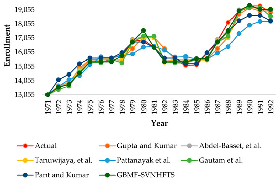
Figure 1.
A graph showing the forecasted values of the historical enrollment data from the GBMF-SVNHFTS method and other FTS methods from 1971 to 1992.

Table 1.
A comparison of the forecasted results of the other FTS methods with the proposed GBMF-SVNHFTS.
Table 2.
A comparison of all three loss functions between the proposed GBMF-SVNHFTS method and other FTS methods.
3.2. Forecasting the Daily Closing Prices of Cryptocurrencies
At the time of this writing, the cryptocurrency market has recently seen the worst decline of any financial market in the world in December 2021. As a result, the data was extremely volatile. To see the performance of the proposed GBMF-SVNHFTS forecasting technique in time series data for the financial sector, we applied it to predict the closing prices of ten major cryptocurrencies with the biggest market capitalization. The descriptive statistics of ten cryptocurrencies are shown in Table 3. To compare the prediction ability of the GBMF-SVNHFTS forecasting technique, we also produced a prediction using the classical ARIMA model [7,8,9], the Sugeno-type ANFIS(S-ANFIS) model [47], and the LSTM model [12]. The training data for our proposed GBMF-SVNHFTS model was the first 70% of the sample, and the latter 30% was used as an out-of-sample dataset for testing the model. We note that a one-step-ahead forecast was used in the out-of-sample forecast.
Table 3.
Ten cryptocurrencies’ data.
To evaluate the forecasting technique, the mean absolute percentage error (MAPE), mean absolute error (MAE), and root mean square error (RMSE) were computed. Table 4 shows the results of our model evaluation and comparison with other methods. Furthermore, we also compared the computation time of the GBMF-SVNHFTS method with the existing models, as shown in Table 5.
Table 4.
A comparison of all three loss functions between the proposed GBMF-SVNHFTS method and existing methods. (Out-of-sample forecasts).
Table 5.
A computation time comparison between the proposed GBMF-SVNHFTS method and existing methods. (sec.).
4. A Forecasting Performance Comparison between the Proposed GBMF-SVNHFTS Method and Other FTS Techniques
The performance in predicting the historical data of the University of Alabama’s student enrollments of the suggested GBMF-SVNHFTS forecasting technique was compared with those of the others proposed by Gupta and Kumar [44], Abdel-Basset, et al. [35], Tanuwijaya, et al. [37], Pattanayak, Panigrahi, and Behera [45], Gautam and Singh [46], and Pant and Kumar [26]. The suggested GBMF-SVNHFTS method has the lowest RMSE, MAPE, and MAE of all the compared FTS models, at 255.7675, 1.0812, and 178.4286, respectively. This means the GBMF-SVNHFTS model has higher accuracy in forecasting student enrollment data than the competing FTS techniques.
Table 4 shows the comparison of the suggested GBMF-SVNHFTS technique with the S-ANFIS method, as well as the ARIMA method and the long short-term memory (LSTM) method, using three loss functions for performance evaluation. To forecast the daily closing prices of ten major cryptocurrencies and compare the results with actual data, we trained the model’s parameters for the S-ANFIS method and built the model’s structure using the Neuro-Fuzzy. For the ARIMA method, we utilized the best fit order to the training dataset and reviewed the residual errors to generate predictions, and compared the outcomes to the test set. In the long short-term memory (LSTM) model, we utilized the Adam optimizer to acquire the neural network parameters, which included two hidden layers, 0.5 dropout, and 200 epochs. To illustrate the out-of-sample performance of all methods, we plot the out-of-sample forecast results in Figure A1.
Moreover, Table 5 shows the computation time results of our method compared to the LSTM, the Sugeno-ANFIS, and the ARIMA methods to illustrate the better performance of our suggested GBMF-SVNHFTS technique on the cryptocurrency dataset. Our technique took the least time in all of the selected ten cryptocurrency datasets except for the DOGE coin, which came as the third best in the least amount of time. Likewise, the proposed GBMF-SVNHFTS method was found to result in the lowest RMSE, MAPE, and MAE of all of the ten major cryptocurrency data series compared with the long short-term memory (LSTM) model, S-ANFIS method, and ARIMA method. This indicates that the GBMF-SVNHFTS approach has more efficiency and accuracy in predicting the daily closing prices of ten major cryptocurrencies than the other methods considered in this study. Furthermore, the ARIMA method is the second-best model among all compared methods for providing the second-best results of all three loss functions of the data from all 10 major cryptocurrencies.
5. Conclusions
This paper aimed to propose a technique to increase the accuracy in time series forecasting since the predictability of the existing FTS techniques has been observed to be not high enough. In our research, we created a single-valued neutrosophic hesitant fuzzy time series forecasting model by combining several of the hesitancy’s degrees. The Gaussian membership function and the bell-shaped membership function were utilized to incorporate the degree of hesitancy to better represent the data movement’s unpredictability, resulting in better forecasting accuracy. The cosine measure and the single-valued neutrosophic hesitant fuzzy weighted geometric (SVNHFWG) operator were used to rank the options and find the optimal one based on the neutrosophic value. We have also demonstrated the efficacy of our GBMF-SVNHFTS method over other fuzzy time series techniques generated from enhanced fuzzy sets.
Two data sets consisting of the short and low-frequency time series data of student enrollment and the long and high-frequency data of ten major cryptocurrencies were used to examine the performance of our method. Using student enrollment as the test data, the results of the comparisons demonstrate that the proposed model is more effective than other FTS models. Moreover, we applied our proposed GBMF-SVNHFTS method to the daily closing prices of the cryptocurrency dataset, which is quite unpredictable, and we compared the outcome to other time series techniques. According to the comparison results, the proposed GBMF-SVNHFTS model outperforms all other time series models in terms of computation time, RMSE, MARE, and MAE. It makes the suggested method more effective at forecasting the future of volatile datasets than other time series techniques. It is recommended that the next study may improve the accuracy of the suggested method by using other types of membership functions or incorporating the meta-heuristic optimization algorithms. Furthermore, the next study may utilize our proposed model for application to other types of datasets, such as stock prices, interest rates, gold, etc. We also suggest applying the belief function approach [48] to improve the prediction interval of the GBMF-SVNHFTS model. Applying this model to predict the histrogram-valued data is also porposed [49].
Author Contributions
Conceptualization, methodology, and software, K.P.; validation, formal analysis, writing—review, and editing, R.T. and W.Y. All authors have read and agreed to the published version of the manuscript.
Funding
The financial support for this work is provided by the Center of Excellence in Econometrics, Chiang Mai University.
Data Availability Statement
The annual student enrollments of the University of Alabama during 1971–1992 can be obtained from the work of [18]. The daily closing prices of ten major cryptocurrencies with the largest market capitalization: Bitcoin (BTC), Ethereum (ETH), Cardano (ADA), Binance Coin (BNB), Dogecoin (DOGE), Solana (SOL), Ripple (XRP), Polygon (MATIC), Polkadot (DOT), and Litecoin (LTC) are collected from www.yahoo.finance.com (accessed on 11 July 2022).
Acknowledgments
The authors would like to thank the two anonymous reviewers and the editor for their helpful comments and suggestions. We would like to express our gratitude to Laxmi Worachai for her help and constant support to us. We thank the Center of Excellence in Econometrics, Faculty of Economics, Chiang Mai University, for financial support.
Conflicts of Interest
The authors declare no conflict of interest.
Appendix A

Figure A1.
The forecasted values from the testing data of ten major cryptocurrency prices from the GBMF-SVNHFTS and other time series techniques.
References
- Lahmiri, S.; Bekiros, S. Cryptocurrency forecasting with deep learning chaotic neural networks. Chaos Solitons Fractals 2019, 118, 35–40. [Google Scholar] [CrossRef]
- Nakamoto, S.; Bitcoin, A. A Peer-To-Peer Electronic Cash System. Available online: https://bitcoin.org/bitcoin.pdf (accessed on 8 July 2022).
- Taskinsoy, J. Bitcoin Could Be the First Cryptocurrency to Reach a Market Capitalization of One Trillion Dollars. Available online: https://ssrn.com/abstract=3693765 (accessed on 8 July 2022).
- Valencia, F.; Gómez-Espinosa, A.; Valdés-Aguirre, B. Price movement prediction of cryptocurrencies using sentiment analysis and machine learning. Entropy 2019, 21, 589. [Google Scholar] [CrossRef] [PubMed]
- Cai, Q.; Zhang, D.; Wu, B.; Leung, S.C. A novel stock forecasting model based on fuzzy time series and genetic algorithm. Procedia Comput. Sci. 2013, 18, 1155–1162. [Google Scholar] [CrossRef]
- Garg, S. Autoregressive integrated moving average model-based prediction of bitcoin close price. In Proceedings of the 2018 International Conference on Smart Systems and Inventive Technology (ICSSIT), Tirunelveli, India, 13–14 December 2018; pp. 473–478. [Google Scholar]
- Yamak, P.T.; Yujian, L.; Gadosey, P.K. A comparison between Arima, lstm, and gru for time series forecasting. In Proceedings of the 2019 2nd International Conference on Algorithms, Computing and Artificial Intelligence, Sanya, China, 20–22 December 2019; pp. 49–55. [Google Scholar]
- Wirawan, I.M.; Widiyaningtyas, T.; Hasan, M.M. Short term prediction on bitcoin price using ARIMA method. In Proceedings of the International Seminar on Application for Technology of Information and Communication (iSemantic), Semarang, Indonesia, 21–22 September 2019; pp. 260–265. [Google Scholar]
- Derbentsev, V.; Datsenko, N.; Stepanenko, O.; Bezkorovainyi, V. Forecasting cryptocurrency prices time series using machine learning approach. SHS Web Conf. 2019, 65, 02001. [Google Scholar] [CrossRef]
- Vapnik, V.; Corinna, C. Support-Vector Networks. Mach. Learn. 1995, 20, 273–297. [Google Scholar]
- Zadeh, L.A. Fuzzy Sets, Fuzzy Sets, Fuzzy Logic, and Fuzzy Systems: Selected Papers by Lotfi A. Zadeh; World Scientific Publishing Co., Inc.: River Edge, NJ, USA, 1996; pp. 394–432. [Google Scholar]
- Hochreiter, S.; Schmidhuber, J. Long short-term memory. Neural Comput. 1997, 9, 1735–1780. [Google Scholar] [CrossRef]
- Zupan, J. Introduction to artificial neural network (ANN) methods: What they are and how to use them. Acta Chim. Slov. 1994, 41, 327. [Google Scholar]
- McNally, S. Predicting the Price of Bitcoin Using Machine Learning. Ph.D. Thesis, National College of Ireland, Dublin, Ireland, 2016. [Google Scholar]
- Lee, L.W.; Wang, L.H.; Chen, S.M. Temperature prediction and TAIFEX forecasting based on high-order fuzzy logical relationships and genetic simulated annealing techniques. Expert Syst. Appl. 2008, 34, 328–336. [Google Scholar] [CrossRef]
- Chen, S.M.; Hwang, J.R. Temperature prediction using fuzzy time series. IEEE Trans. Syst. Man Cybern. Part B (Cybern.) 2000, 30, 263–275. [Google Scholar] [CrossRef]
- Vamitha, V.; Jeyanthi, M.; Rajaram, S.; Revathi, T. Temperature prediction using fuzzy time series and multivariate Markov chain. Int. J. Fuzzy Math. Syst. 2012, 3, 217–230. [Google Scholar]
- Song, Q.; Chissom, B.S. Forecasting enrollments with fuzzy time series—Part I. Fuzzy Sets Syst. 1993, 54, 1–9. [Google Scholar] [CrossRef]
- Chen, S.M. A new method to forecast enrollments using fuzzy time series. Int. J. Appl. Sci. Eng. 2004, 2, 234–244. [Google Scholar]
- Huarng, K. Effective lengths of intervals to improve forecasting in fuzzy time series. Fuzzy Sets Syst. 2001, 123, 387–394. [Google Scholar] [CrossRef]
- Chen, S.M. Forecasting enrollments based on high-order fuzzy time series. Cybern. Syst. 2002, 33, 1–16. [Google Scholar] [CrossRef]
- Yu, H.K. A refined fuzzy time-series model for forecasting. Phys. A Stat. Mech. Its Appl. 2005, 346, 657–681. [Google Scholar] [CrossRef]
- Liu, H.T. An improved fuzzy time series forecasting method using trapezoidal fuzzy numbers. Fuzzy Optim. Decis. Mak. 2007, 6, 63–80. [Google Scholar] [CrossRef]
- Pattanayak, R.M.; Behera, H.S.; Panigrahi, S. A non-probabilistic neutrosophic entropy-based method for high-order fuzzy time-series forecasting. Arab. J. Sci. Eng. 2022, 47, 1399–1421. [Google Scholar] [CrossRef]
- Singh, P.; Huang, Y.P. A new hybrid time series forecasting model based on the neutrosophic set and quantum optimization algorithm. Comput. Ind. 2019, 111, 121–139. [Google Scholar] [CrossRef]
- Pant, M.; Kumar, S. Fuzzy time series forecasting based on hesitant fuzzy sets, particle swarm optimization and support vector machine-based hybrid method. Granul. Comput. 2022, 7, 861–879. [Google Scholar] [CrossRef]
- Atanassov, K. Intuitionistic fuzzy sets. Fuzzy Sets Syst. 1986, 20, 87–96. [Google Scholar] [CrossRef]
- Joshi, B.P.; Kumar, S. Intuitionistic fuzzy sets based method for fuzzy time series forecasting. Cybern. Syst. 2012, 43, 34–47. [Google Scholar] [CrossRef]
- Torra, V.; Narukawa, Y. On hesitant fuzzy sets and decision. In Proceedings of the IEEE International Conference on Fuzzy Systems, Jeju Island, Korea, 20–24 August 2009; pp. 1378–1382. [Google Scholar]
- Torra, V. Hesitant fuzzy sets. Int. J. Intell. Syst. 2010, 25, 529–539. [Google Scholar] [CrossRef]
- Zhu, B.; Xu, Z.; Xia, M. Dual hesitant fuzzy sets. J. Appl. Math. 2012, 2012, 879629. [Google Scholar] [CrossRef]
- Bisht, K.; Kumar, S. Fuzzy time series forecasting method based on hesitant fuzzy sets. Expert Syst. Appl. 2016, 64, 557–568. [Google Scholar] [CrossRef]
- Smarandache, F. A unifying field in Logics: Neutrosophic Logic. In Philosophy; American Research Press: Santa Fe, NM, USA, 1999; pp. 1–141. [Google Scholar]
- Wang, H.; Smarandache, F.; Zhang, Y.; Sunderraman, R. Single Valued Neutrosophic Sets; Infinite Study: Coimbatore, India, 2010. [Google Scholar]
- Abdel-Basset, M.; Chang, V.; Mohamed, M.; Smarandache, F. A refined approach for forecasting based on neutrosophic time series. Symmetry 2019, 11, 457. [Google Scholar] [CrossRef]
- Ye, J. Multiple-attribute decision-making method under a single-valued neutrosophic hesitant fuzzy environment. J. Intell. Syst. 2015, 24, 23–36. [Google Scholar] [CrossRef]
- Tanuwijaya, B.; Selvachandran, G.; Abdel-Basset, M.; Huynh, H.X.; Pham, V.H.; Ismail, M. A novel single valued neutrosophic hesitant fuzzy time series model: Applications in Indonesian and Argentinian stock index forecasting. IEEE Access 2020, 8, 60126–60141. [Google Scholar] [CrossRef]
- Vaidya, A.V.; Metkewar, P.S.; Naik, S.A. A new paradigm for generation of fuzzy membership function. In Proceedings of the 2018 IEEE 8th International Advance Computing Conference (IACC), Greater Noida, India, 14–15 December 2018; IEEE: Piscataway, NJ, USA, 2018; pp. 1–6. [Google Scholar]
- Maturo, F.; Fortuna, F. Bell-shaped fuzzy numbers associated with the normal curve. In Topics on Methodological and Applied Statistical Inference; Springer: Cham, Switzerland, 2016; pp. 131–144. [Google Scholar]
- Reddy, C.S.; Raju, K.V. An Improved Fuzzy Approach for COCOMO’s Effort Estimation Using Gaussian Membership Function. J. Softw. 2009, 4, 452–459. [Google Scholar] [CrossRef]
- Zimmermann, H.J. Fuzzy Set Theory—And Its Applications; Springer Science & Business Media: Berlin/Heidelberg, Germany, 2011. [Google Scholar]
- Giachetti, R.E.; Young, R.E. A parametric representation of fuzzy numbers and their arithmetic operators. Fuzzy Sets Syst. 1997, 91, 185–202. [Google Scholar] [CrossRef]
- Zhao, J.; Bose, B.K. Evaluation of membership functions for fuzzy logic controlled induction motor drive. In Proceedings of the IEEE 2002 28th Annual Conference of the Industrial Electronics Society, Seville, Spain, 5–8 November 2002; Volume 1, pp. 229–234. [Google Scholar]
- Gupta, K.K.; Kumar, S. Hesitant probabilistic fuzzy set based time series forecasting method. Granul. Comput. 2019, 4, 739–758. [Google Scholar] [CrossRef]
- Pattanayak, R.M.; Panigrahi, S.; Behera, H.S. High-order fuzzy time series forecasting by using membership values along with data and support vector machine. Arab. J. Sci. Eng. 2020, 12, 10311–10325. [Google Scholar] [CrossRef]
- Gautam, S.S.; Singh, S.R. A modified weighted method of time series forecasting in intuitionistic fuzzy environment. Opsearch 2020, 57, 1022–1041. [Google Scholar] [CrossRef]
- Sugeno, M. An introductory survey of fuzzy control. Inf. Sci. 1985, 36, 59–83. [Google Scholar] [CrossRef]
- Yamaka, W.; Sriboonchitta, S. Forecasting Using Information and Entropy Based on Belief Functions. Complexity 2020, 2020, 3269647. [Google Scholar] [CrossRef]
- Maneejuk, P.; Pirabun, N.; Singjai, S.; Yamaka, W. Currency Hedging Strategies Using Histogram-Valued Data: Bivariate Markov Switching GARCH Models. Mathematics 2021, 9, 2773. [Google Scholar] [CrossRef]
Publisher’s Note: MDPI stays neutral with regard to jurisdictional claims in published maps and institutional affiliations. |
© 2022 by the authors. Licensee MDPI, Basel, Switzerland. This article is an open access article distributed under the terms and conditions of the Creative Commons Attribution (CC BY) license (https://creativecommons.org/licenses/by/4.0/).