Abstract
A discrete modified Leslie–Gower prey-predator model considering the effect of fear on prey species is proposed and studied in this paper. First, we discuss the existence of equilibria and the local stability of the model. Second, we use the iterative method and comparison principle to obtain the set of conditions which ensures the global attractivity of positive equilibrium point. The results show that prey and predator can coexist stably when the intrinsic growth rates of both prey and predator are maintained within a certain range. Then, we study the global attractivity of the boundary equilibrium point. Our results suggest that when the intrinsic rate of prey is small enough or the fear factor is large enough, the prey will tend to go extinct, while the predator can survive stably due to the availability of other food sources. Subsequently, we discuss flip bifurcation, transcritical bifurcation at the equilibria of the system, by using the center manifold theorem and bifurcation theory. We find that system changes from chaotic state to four-period orbit, two-period orbit, stable state, and finally prey species will be driven to extinction, while predator species survive in a stable state for enough large birth rate of prey species with the increasing of fear effect. Finally, we verify the feasibility of the main results by numerical simulations, and discuss the influence of the fear effect. The results show that the fear effect within a certain range can enhance the stability of the system.
Keywords:
Leslie–Gower predator–prey system; fear effect; discrete-time; flip bifurcation; transcritical bifurcation; global attractivity MSC:
92D25; 34D20
1. Introduction
The dynamic quantitative relationship between predator and prey has always been a hot topic in ecology and mathematical ecology. The derivation of more realistic predator–prey dynamics models is a major trend of relevant theoretical research. Traditionally, all predator–prey models evolve from two basic models—the first is the famous Lotka–Volterra predator–prey model [1], which takes the form
In this model, is the transform rate of the predator species. A total of prey populations are captured, and the energy gained by the predator will further generate individuals in the predator population. The model can be adjusted to a more suitable predator–prey model by incorporating functional response, which takes the form
There are numerous kinds of functional response, depending on the circumstance considered. These include the Holling II functional response [1], Beddington–DeAngelis functional response [2] and square root functional response [3], etc.
The second one is now referred to as the Leslie–Gower predator–prey model, which was first introduced by Leslie [4], where the carrying capacity of the predator’s environment is proportional to the number of prey:
The model seems very simple, however, only in 2001 did Korobeinikov [5] give a strict proof of the global stability property of the positive equilibrium. Since then, numerous studies had been conducted in this direction. For example, Chen, Chen, and Xie [6] incorporated prey refuge in the system (3) and showed that refuge has a complicated influence on the dynamic behaviors of the predator species. To investigate the influence of human disturbance, Chen and Chen [7] proposed a Leslie–Gower predator–prey model with feedback control; by constructing a suitable Lyapunov function, they obtained a set of sufficient conditions which ensured the existence of a unique globally asymptotically stable positive equilibrium of the system. Li, Han, and Chen [8] studied the stability property of the stage-structured predator–prey model. Recently, several scholars [9,10,11,12] studied the influence of Allee effect on the Leslie–Gower predator–prey system. They gave a detailed bifurcation analysis of the model proposed. Yu and Chen [13] and Yu [14] studied the mutual interferences of the predator species. Zhu and Kong [15] showed that nonlinear harvesting may lead to very complicated dynamic behaviors in the system. Zou and Guo [16] studied the influence of a spatially heterogeneous environment on a diffusive Leslie–Gower predator–prey model. Mondal, Pal, and Samanta [17] proposed a Leslie–Gower predator–prey eco-epidemiological model with disease in predator; they gave a thorough analysis of the dynamic behaviors of the system. Liang, Zeng, Pang, and Liang [18] showed that a Leslie–Gower predator–prey system with ratio-dependent and state impulsive feedback control could have a periodic solution, which is quite different from the dynamic behaviors of the system (3).
Aziz-Alaoui and Okiye [19] proposed a modified Leslie–Gower predator–prey model in 2003. The authors argued that in the case of severe scarcity, a predator species can switch over to other populations, but its growth will be limited by the fact that its favorite food (prey species) is not available in abundance. The modified Leslie–Gower predator–prey model with Holling I functional response can be described by the following equations:
where and represent the population density of the prey population and the predator population at time t, respectively; m represents the environmental protection rate for predators, which reflects the fact that the predators have other food resources; r represents the birth rate of the predator population; and f represents the mortality of the predator population due to intraspecific competition. Wu [20] further incorporated prey refuge to above system, and he showed that under some suitable assumption, the system may exist a unique positive equilibrium. The condition which ensure the existence of the positive equilibrium is enough to ensure its globally asymptotically stability.
Considering that the population of predators can not only directly reduce the population density of the prey species by catching prey as its food resource, the presence of predators creates fear in the prey species because the prey species is always alert to potential attacks, and the prey will engage in reverse feeding behavior in response to the perceived risk (e.g., foraging frequency decreases and decreased number of offspring foraging), which leads to a decrease in the prey species population density. The fear response of prey is called the fear effect. The first famous experiment was done by Zanette, White, Allen, and Clinchy [21]. They experimented on song sparrows over the course of an entire breeding season to see if perceived predation danger could, even in the absence of direct killing, influence reproduction. They discovered that having a fear of predators caused the number of offspring to reduce by 40%.
In 2016, based on system (1), Wang, Zanette and Zou [22] first proposed a continuous predator–prey model incorporating the fear effect:
where and represent the population density of the prey population and the predator population at time t, respectively. k represents the level of fear that drives the anti-predatory behavior of prey, and d represent the birth rate and natural mortality rate of the prey population, respectively, a represents the mortality of the prey population due to intraspecific competition, and b represents maximum capture rate of predators. The authors showed that for system (5), fear effect had no influence on the existence or stability of the equilibria.
Zhu, Wu, Lai et al. [23] proposed the following predator–prey model:
In this model, without the prey species, the predator species takes the form
It is a logistic equation, which means that in system (6), the authors made the assumption that the predator species takes other species as food resources. Their study showed that the fear effect is one of the most important factors leading to the extinction of the prey species. This result is quite different from the results of Wang, Zanette and Zou [22].
It is natural to study the influence of the fear effect in the Leslie–Gower-type predator–prey system; indeed, many scholars [9,10,24,25,26] have conducted research in this direction. Firdiansyah [24] employed a Leslie–Gower predator–prey model with Beddington–DeAngelis functional response to examine the influence of fear effect; the model had the following form:
The author demonstrated that an increase in fear might reduce the population density of both species. However, in the event of a constant fear rate, prey refuge is beneficial to the survival of both species. For more works on continuous predator–prey models incorporating the fear effect, one could refer to [22,23,24,25,26,27,28,29,30,31,32,33,34,35,36,37,38] and the references cited therein.
It is well-known that when species have non-overlapping generations or their population sizes are too small, discrete models described by difference equations are more appropriate than continuous-time ones. Generally speaking, discrete systems will have more complex dynamical behaviors. However, to this day, there are not many works on discrete predator–prey systems incorporating the fear effect.
Corresponding to system (5), Kundu, Pal, and Samanta [34] proposed the following discrete predator–prey system with consideration of fear effect in prey species:
The dynamic behaviors of this system are quite different from those of the system (5). Indeed, the authors showed that the stability of the coexistence equilibrium point of the corresponding discrete-time model changed (unstable to stable) with the increase of the cost of fear k.
Stimulated by the work of Wang, Zanette, and Zou [22]; Zhu, Wu, Lai et al. [23]; and Kundu, Pal, and Samanta [34], corresponding to system (6), Chen, He, and Chen [35] recently proposed and studied a discrete predator–prey model, in which the prey population has a fear effect and the predator population has other food sources:
The authors paid attention to the local and global stability property of the equilibria of the system. They showed that due to the fear of predation, the prey species will be driven to extinction while the predator species tends to be stable since it has other food resources.
Given this background, it is natural to propose a discrete Leslie–Gower discrete predator–prey model with fear effect in prey species, and to study the influence of fear effect. In this paper, based on the model (4), we propose the following discrete Leslie–Gower predator–prey model:
where and are the population density of prey and predator at the nth-generation, respectively. k represents the level of fear that drives the anti-predatory behavior of prey, and d represent the birth rate and natural mortality rate of the prey population, respectively, a represents the mortality of the prey population due to intraspecific competition, b represents the maximum capture rate of predators, and h represents the intrinsic growth rate of predators. m represents the environmental protection rate for predators, which reflects the fact that the predators have other food resources. , k, d, a, b, h, and m are all positive constants. Since there seems to be no research on discrete Leslie–Gower predator–prey systems with fear effect, this study would be an interesting attempt to complement existing research on Leslie–Gower predator–prey systems.
As far as system (11) is concerned, there are several issues needing to be solved: (1) Is it possible to give a thorough analysis of the local and global stability of the equilibrium? (2) Is it possible to investigate the bifurcation phenomenon of the system? (3) To what extent does fear effect k change the dynamic behaviors of the system?
We investigate these three issues in this paper. The rest of the paper is arranged as follows: We investigate the existence, local stability, and global stability of equilibria in Section 2, Section 3 and Section 4, respectively. We then investigate the bifurcation phenomenon in Section 5. Some numerical simulations are carried out to show the feasibility of the main results in Section 6. We end this paper with a brief discussion.
2. The Existence of Equilibria
The equilibria of system (11) are determined by the following equations:
By solving Equation (12), we can obtain the following conclusions:
Theorem 1.
System (11) always has two boundary equilibria given by ; if holds, there is also a boundary equilibrium .
Theorem 2.
Assuming that
holds, system (11) admits a unique positive equilibrium , where , is the unique positive solution of the equation:
with
Proof.
Since , Equation (12) is equivalent to:
The second equation of (16) is equivalent to . Substituting it into the first equation and simplifying it, we obtain Equation (14). Obviously, both and are positive, so Equation (14) has a unique positive solution if and only if , i.e., . Consequently, the system (11) has a unique positive equilibrium , where
The proof of Theorem 2 is finished. □
Remark 1.
One could easily see that (14) has no positive solution, consequently, if condition (13) does not hold, the system (11) does not admit any positive equilibrium. So we can draw the following conclusions:
The equilibria of the system (11) are:
- (1)
- , , if ;
- (2)
- , , and , if ;
- (3)
- , , , and , if .
Remark 2.
Assume is the unique positive root of Equation (14), i.e.,
where . Computing the derivative of (17) with respect to k, we obtain
where "" represents the derivative . Simple calculation and analysis can reveal that
which means that the value of prey equilibrium is strictly deceasing function of k.
Due to
we can conclude that the value of predator equilibrium is also is the decreasing function of k,however,
3. The Local Stability of Equilibria
The Jacobian matrix of system (11) at the equilibrium is
Next, we judge the local stability of the equilibria of system (11) according to the above Jacobian matrix and Lemmas 1 and 2 in [35].
3.1. The Local Stability of Boundary Equilibria
Theorem 3.
is
- (1)
- A source if ;
- (2)
- A saddle if ;
- (3)
- Non-hyperbolic if .
Proof.
The Jacobian matrix of system (11) at is
Obviously, the two eigenvalues of are and Hence, if , i.e., , then is a source according to Lemma 1 of [35]. Thus, (1) holds. Numbers (2) and (3) can be proved in the same way. Therefore, is always unstable.
The proof of Theorem 3 is finished. □
Theorem 4.
is
- (1)
- A sink if and ;
- (2)
- A source if and ;
- (3)
- A saddle if one of the following conditions holds:
- (i)
- and ;
- (ii)
- and ;
- (4)
- Non-hyperbolic if or .
Proof.
The Jacobian matrix of system (11) at is
the two eigenvalues of are and Hence, if and , we have and , then is a sink according to Lemma 1 of [35]. Thus, (1) holds, and (2)–(4) can be proved in the same way. Therefore, is stable if and only if and .
The proof of Theorem 4 is finished. □
Theorem 5.
If the predator-free equilibrium of system (11) exists (i.e., holds), we can easily obtain that is
- (1)
- A source if ;
- (2)
- A saddle if ;
- (3)
- Non-hyperbolic if .
Proof.
The Jacobian matrix of system (11) at is
Obviously, the two eigenvalues of are and . Similar to the proof in Theorem 4, the above results can be easily obtained.
The proof of Theorem 5 is finished. □
3.2. The Local Stability of the Positive Equilibrium
Theorem 6.
If the positive equilibrium of system (11) exists, i.e., , we can easily obtain that is
- (1)
- A sink if or ;
- (2)
- A source if one of the following conditions holds:
- (i)
- and ;
- (ii)
- and ;
- (3)
- A saddle if and ;
- (4)
- Non-hyperbolic if , where
Hence, is locally asymptotically stable if or ; otherwise, it is unstable.
Proof.
The Jacobian matrix of system (11) at is
Therefore, the characteristic equation of is , where
If or holds, then , . Hence, according to Lemmas 1 and 2 in [35], we obtain that is a sink, which is stable. Numbers (2)–(4) can be proved in the same way.
The proof of Theorem 6 is finished. □
4. The Global Attractivity of Equilibria
4.1. The Global Attractivity of the Positive Equilibrium
According to Theorem 6, the positive Equilibrium is locally asymptotically stable when or . Next, we further explore global attractivity by using Lemmas 3–5 from [35].
Theorem 7.
If and , the positive equilibrium is globally attractive, i.e.,
where , , ε is an arbitrarily small positive number.
Proof.
Let be any positive solution of system (11) with and . Let
Therefore, to prove (19), we need only prove the following equations:
If there exist four sequences , , , satisfying:
and
then Equation (20) is clearly established according to the squeezing of the limit. Below, we construct these four sequences by the iterative method:
- (I)
- Through the first iteration, we can prove that there exist , such that and .
- (i)
- Given by the first equation of system (11), we getConsider the auxiliary equationsince , we obtain for all , where is any solution of system (23) with according to Lemma 3 in [35]. From Lemma 4 in [35], we have is nondecreasing for . Hence, according to Lemma 5 in [35], we have that for all , where is any solution of (23) satisfying the initial condition . Furthermore, because , we have according to Lemma 3 in [35]. Therefore, we haveHence, for sufficiently small there exists an integer such that if , then
- (ii)
- Given by the second equation of system (11), we getConsider the auxiliary equationSince , we obtain that for all from Lemma 3 in [35]. According to Lemma 4 in [35], we have that is nondecreasing for . Hence, according to Lemma 5 in [35], we have that for all . Therefore, as with (I) (i), we getHence, for sufficiently small there exists an integer such that if , then
- (II)
- Through the second iteration, we can prove that there exist , such that and .
- (i)
- Given by the first equation of system (11), we obtain thatConsider the auxiliary equationSince , we obtainHence for all according to Lemma 3 in [35]. From Lemma 4 in [35], we know that is nondecreasing for . Hence, according to Lemma 5 in [35], we have that for all . According to Lemma 3 in [35], we haveHence, for sufficiently small , there exists an integer such that if , then
- (ii)
- Given by the second equation of system (11), we obtainConsider the auxiliary equationSince , with a similar argument as above, we can obtainHence, for sufficiently small there exists an integer such that if , then
- (III)
- Through the third iteration, we can prove that there exist , such that and .
- (i)
- Given by the first equation of system (11), we obtain thatSince , we obtain , according to Lemma 5 in [35], we have thatHence, for sufficiently small , there exists an integer such that if , then
- (ii)
- Given by the second equation of system (11), we obtainSince , with a similar argument as above, we can obtainHence, for sufficiently small , there exists an integer such that if , then
- (IV)
- Through the fourth iteration, we can prove that there exist , such that and .
- (i)
- Similarly, from the first equation of system (11), we obtainSince , we can obtainAccording to Lemma 5 in [35], we haveHence, for sufficiently small there exists an integer such that if , then
- (ii)
- Similarly, from the second equation of system (11), we obtainSince , with a similar argument as above, we can obtainHence, for sufficiently small there exists an integer such that if , then
By repeating steps (III)–(IV), sequences , , , , are constructed as follows (define as 0):
These four sequences clearly satisfy inequalities (21), and it is shown below that they also satisfy equalities (22).
We first prove that the limits of all four sequences exist, which can be proved by using the monotone bounded criterion of sequence. First, it is proved by mathematical induction that all four sequences are monotone, and that and are monotonically decreasing, while and are monotonically increasing.
Obviously, if , we have
For (), we assume that and hold. Then, further, we have
Consequently,
Therefore, these four sequences are all monotone by mathematical induction. Combining with inequalities (21), it is easy to obtain that sequences and have lower bounds and monotonic decreasing, and sequences and have upper bounds and monotonic increasing. Therefore, it can be known from the monotone bounded criterion that the limits of these four sequences all exist. Let
Obviously, they are all positive. Then, it is only necessary to prove that , .
Let us take the limit of both sides of the equality sign of the four equations in (25); taking , we obtain
Note that the system of Equation (27) is equivalent to (16) if , and , so it can be known from and from Theorem 2 that the positive equilibrium exists at this time, and therefore the system of Equation (27) has a positive solution under the assumption of Theorem 7. Following we will prove that the positive solution of the system (27) is unique.
The following can be obtained by simplification of (27):
Similarly, we know that (28) has at least one positive solution . Below, we prove that Equation (28) has only one positive solution:
Otherwise, Equation (28) has other positive solutions, that is, there are positive numbers satisfying (28). Subtracting the first equation of (28) from the second equation, we obtain
Because , it can be obtained from (29) that
Since , we have , which contradicts the fact that both and are positive.
Hence, Equation (28) has only one positive solution . Then, we have from (27). Thus, we prove that these four sequences also satisfy the equalities (22). Therefore, the positive equilibrium is globally attractive.
The proof of Theorem 7 is finished. □
4.2. The Global Attractivity of the Boundary Equilibrium
In the previous section, we proved that the positive equilibrium is globally attractive under certain conditions, which indicates that predator and prey populations can coexist stably under certain conditions. When the prey population goes extinct, the predator population probably does not go extinct with it, and tends to stabilize because there are other food sources. This section discusses this possibility, and proves that the boundary equilibrium is also globally attractive under certain conditions.
Theorem 8.
If , any positive solution of system (11) is ultimately bounded.
Proof.
Therefore, for any sufficiently small there exists an integer such that if , then
According to Lemma 6 in [35], we have
Therefore, for any sufficiently small there exists an integer such that if , then
Combining (30) and (31), it can be concluded that any positive solution of system (11) is ultimately bounded.
The proof of Theorem 8 is finished. □
Next we use Lemmas 6 and 7 from [35] and Theorem 8 to discuss the global attractivity of .
Theorem 9.
Assuming that
and
hold, the boundary equilibrium is globally attractive, i.e.,
where is any positive solution of system (11).
Proof.
Assume that is any positive solution of system (11). First let us prove that .
From (32), we have
Hence, there exist the positive constants p and q such that
Then,
and
Then, there exists such that
Adding both sides from 0 to , we have
then
Hence, with , i.e.,
Therefore, for any sufficiently small , there exists an integer such that if , then
Then, we prove that
Consider the system:
The system has a unique positive equilibrium . Let be any positive solution of system (40); from (33), so can be obtained by applying Lemma 3 in [35]. Therefore, to prove that , we need only prove that
Assume that
then, we only need to prove .
Substituting (39)–(41) into the second equation of system (11), we can obtain the following equation by simple calculation:
where , which means .
Since , from Lemmas 6 and 7 in [35], we obtain
According to system (40), we obtain
Therefore, for any sufficiently small , there exists an integer such that
Let
since is sufficiently small, we obtain
Given (45) and because is sufficiently small, we can obtain from the above inequality.
The proof of Theorem 9 is finished. □
5. Bifurcation Analysis
In this section, we discuss bifurcations at the equilibria of the system (11). We can easily derive the following theorems by using the central manifold and bifurcation theory [37,38].
5.1. Flip Bifurcation
First, we discuss the flip bifurcation of the system (11) at .
Theorem 10.
System (11) undergoes flip bifurcation at if parameters vary in the small neighborhood of .
Theorem 11.
System (11) undergoes flip bifurcation at if parameters vary in the small neighborhood of .
Proof.
The proof of Theorem 11 is similar to the proof of Theorem 10. Therefore, we only give the proof of Theorem 10. First, we can obtain that if and hold, the eigenvalues of are and . Since a center manifold of system (11) at is and the system (11) restricted to it is the logistic model:
Its nontrivial fixed point is . Then, we can easily obtain that
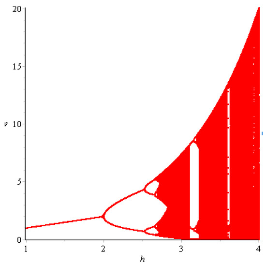
when parameters vary in the small neighborhood of . Hence, flip bifurcation can occur at , as shown in Figure 1.
Figure 1.
Flip bifurcation diagram of the boundary fixed point .
The proof of Theorem 10 is finished. □
5.2. Transcritical Bifurcation
In this section, our claim is that fixed point undergoes transcritical bifurcation.
Theorem 12.
System (11) undergoes transcritical bifurcation at its trivial equilibrium if parameters vary in the small neighborhood of .
Proof.
First, we can obtain that if and hold, the eigenvalues of are and .
As , we can describe system (11) by the following map:
where and parameter represents a very small perturbation parameter such that . If we expand the system (47) by Taylor at , we have:
where
Therefore, there exists a center manifold for map (48) at in a small neighborhood of :
Then, h must satisfy
h can be written as
Substituting (50) into (49), we can obtain . Additionally, the map restricted to the center manifold is given by:
Next, we establish and as follows:
Thus, we can state that system (11) undergoes transcritical bifurcation at if .
The proof of Theorem 12 is finished. □
6. Numerical Simulations
In this section, we show the feasibility of the main results of this paper. Through numerical simulation, we directly analyze the influences of fear effect on discrete system (11).
Example 1.
The stability of the positive equilibrium .
- (1)
- Whenwe take the initial values of system (11) as , we have , then the system (11) admits a unique positive equilibrium according to Theorem 2. At this point, we have , then is locally asymptotically stable according to Theorem 6, as shown in Figure 2. In fact, if we take the initial values of system (11) as , we can see that is also globally stable in Figure 3, but at this point we have . It shows that it is possible for to be globally attractive even if the conditions of Theorem 7 are not satisfied. This means that sufficient conditions to ensure the globally asymptotically stable equilibrium is too strict, which is probably due to the contraction and expansion of the proof.
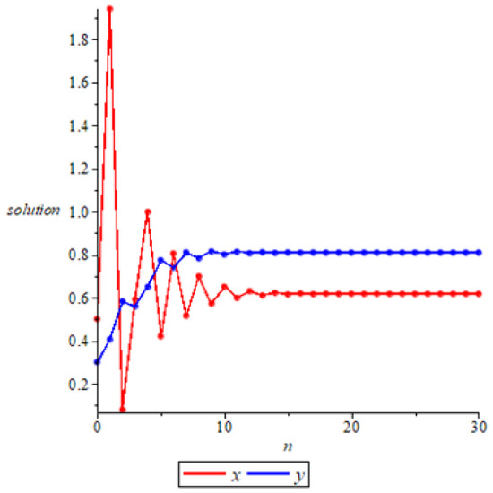 Figure 2. Local stability of positive equilibrium .
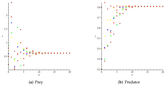 Figure 3. Global attractivity of positive equilibrium .
 - (2)
- Whenand , we have , the system (11) has a unique positive equilibrium according to Remark 3. At this point, we have , then is a saddle according to Theorem 6, as shown in Figure 4.
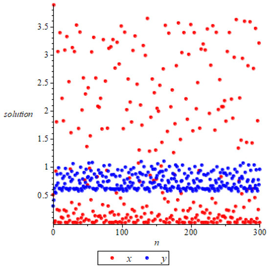 Figure 4. The positive equilibrium is unstable.
Example 2.
The stability of prey-free equilibrium .
- (1)
- Whenand , we have and , then is locally asymptotically stable according to Theorem 4, as shown in Figure 5. Further, we can see that and , which means that is globally attractive according to Theorem 9. We take the initial values of the system (11) as
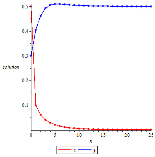 Figure 5. Local stability of prey-free equilibrium.respectively, for numerical simulation, and the results verify the accuracy of the conclusion of Theorem 9, as shown in Figure 6.
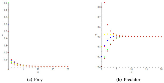 Figure 6. Global attractivity of prey-free equilibrium.
 - (2)
- Whenwe haveand , which satisfy the conditions of Theorem 4, but do not meet the requirements of Theorem 9. However, we take the initial values of the system aswe can see that is also globally attractive at this time from Figure 7.
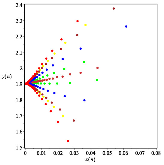 Figure 7. The prey-free equilibrium is also globally attractive at this time.
Example 3.
The impact of fear effect on system stability is studied by numerical simulations.
- (1)
- First, we consider the case where there is no fear effect. Set each parameter value of system (11) as and set . Through numerical simulation, we find that when , system (11) has a stable equilibrium point. When continues to increase, this equilibrium point first bifurcates into a two-period orbit (), then bifurcates into a four-period orbit (), and finally chaos occurs (), as shown in Figure 8. We can see that with the increasing of grow rate of prey species, the dynamic behaviors of both predator and prey becomes complicated.
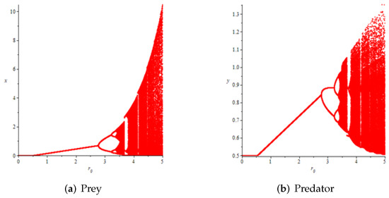 Figure 8. Variation of prey and predator densities with parameter ().
 - (2)
- Then, we consider the fear effect. Set each parameter value of system (11) as:set , and plot with k as the abscissa. We can see from Figure 9 that the system (11) changes from chaotic state () to eight-period orbit (), four-period orbit (), then to two-period orbit (), to stable state (), and finally to be the state that the prey is driven to extinction while the predator survive in a stable state (). This means that the stability of system (11) increases as the fear effect of prey increases within a certain range, which is similar to the result in [35]. In addition, it can be seen from Figure 9 (c)-(d) that the positive equilibrium solution of the system (11) will decrease with the increasing of k, which is consistent with the conclusion of Remark 2. If k is sufficiently large, the prey will become extinct, while the predator will not become extinct due to the presence of other food sources.
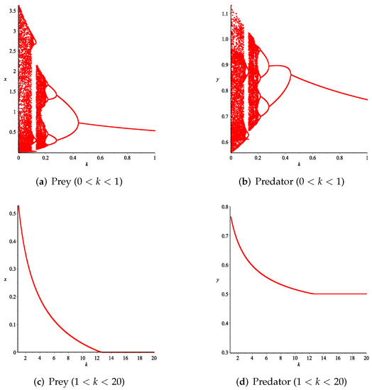 Figure 9. Variation of prey and predator densities with parameter k.The phase portraits correlated with Figure 9 are displayed in Figure 10, which includes orbits of periods 2, 4, and 8. When , we can see chaotic sets in Figure 10a.
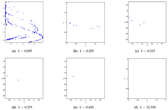 Figure 10. Phase portraits for various values of k corresponding to Figure 9.
Example 4.
The influence of fear effect on the positive equilibrium solution of system.
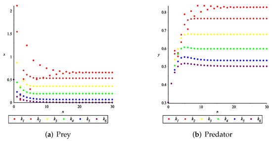
Set each parameter value of system (11) as:
and . The fear effect values were set as
for numerical simulation, and the number of iterations n was taken as the abscissa for plotting, as shown in Figure 11. It can be seen from Figure 11 that the larger the fear effect is, the smaller the positive equilibrium solution is. In other words, the density of prey and predator population in the stable state will decrease with the increasing of the fear effect. When the fear effect is sufficiently large, the prey population will become extinct, while the predator population will become stable. In addition, it is noted that when the fear effect is in a certain range, the larger the fear effect is, the fewer iterations it takes for the predator and prey populations to stabilize, that is, the faster the two populations stabilize. Therefore, it is concluded that the fear effect k can enhance the stability of the positive equilibrium solution and reduce the value of the positive equilibrium solution , which is consistent with the conclusion of Remark 2 and Figure 9c,d.
Figure 11.
Prey and predator densities at different values of k.
Example 5.
The impact of fear effect and other food resource on system stability is studied by numerical simulations.
- (1)
- First, we consider the case where there is no fear effect and has the variable other food resource. Set each parameter value of system (11) as and set . Depending on , , and , we give the corresponding numerical simulations (Figure 12, Figure 13, Figure 14 and Figure 15). We found that in any cases, too many other food sources can accelerate the demise of prey populations. The possible reason is that with the increasing of other food sources, the number of predator populations has increased. Therefore, although the influence of a single predator on the prey is reduced, the overall predator population will have an excessive impact on the prey population, which will lead to the decreasing of the prey population, and finally the prey species will be driven to extinction.
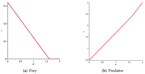 Figure 12. Variation of prey and predator densities with parameter m ().
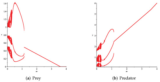 Figure 13. Variation of prey and predator densities with parameter m ().
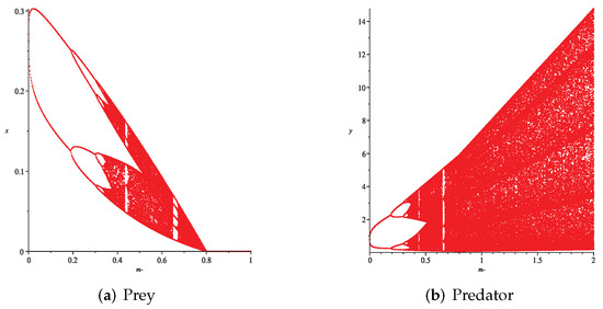 Figure 14. Variation of prey and predator densities with parameter m ().
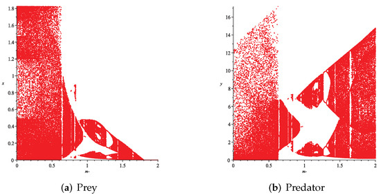 Figure 15. Variation of prey and predator densities with parameter m ().
 - (2)
- Then, we consider the influence of fear effect. Set each parameter value of system (11) as:set , and plot with k as the abscissa. Corresponding to the four cases discussed above, we choose suitable m, such that two species could be coexist, no matter in the stable state or chaos state. Figure 16, Figure 17, Figure 18 and Figure 19 show that in any cases, if the fear effect is too large, the prey species will be driven to extinction, while depending on the intrinsic growth rate of predator species, the predator species will state in stable state for the case , and in chaos state for the case .
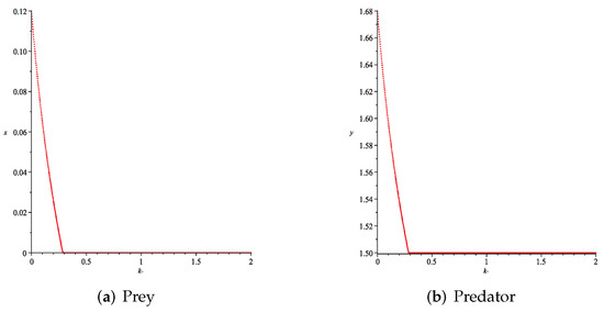 Figure 16. Variation of prey and predator densities with parameter k ().
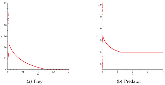 Figure 17. Variation of prey and predator densities with parameter k ().
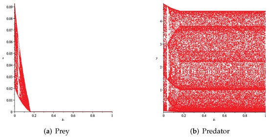 Figure 18. Variation of prey and predator densities with parameter k ().
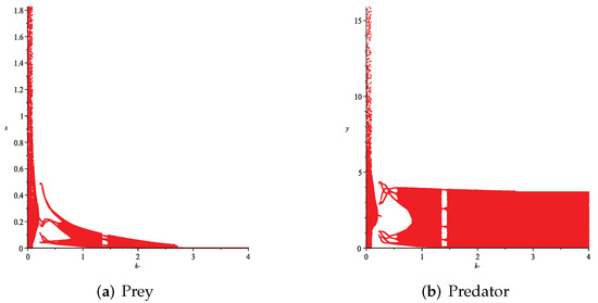 Figure 19. Variation of prey and predator densities with parameter k ().
7. Discussion
Based on the traditional Lotka-Volterra predator prey model, Wang, Zanette, and Zou [22] proposed system (5), in which the authors argued that the fear effect of predator to prey may reduce the birth rate of the prey species. Their studied indicated that if the system exists a positive equilibrium, it then is globally asymptotically stable. since the existence condition is independent of the fear effect, one could draw the conclusion that fear effect has no influence to the dynamic behaviors of the system (5). One may conjecture that such a property still hold for the discrete counterpart system, however, Kundu, Pal, Samanta, and Sen [34] showed that for system (9), the situations become complicated. If the birth rate of the prey species is enough large, then, without the influence of fear effect, both predator and prey species may have chaotic behaviors, then, for fixed birth rate, with the increasing of fear effect, the system could becomes stable. They then drew the conclusion “fear effect enhances stability in a predator-prey system”. However, an amazing property about system (9) is that the system may have Hopf bifurcation, as was shown in Theorem 4.1 and Figure 5 in [34]. The existence of Hopf bifurcation exclude the global asymptotically stability of the positive equilibrium, since such kind of phenomenon is induced by fear effect, we think the fear effect also have negative effect on the stability of the system.
Zhu, Wu, Lai and Yu [23] proposed system (6), in which the predator species has other food resource, they showed that the fear effect is one of the most important factors that lead to the extinction of the prey species. The authors of [23] only paid attention to the influence of fear effect, the dynamic behaviors of system (5) and (6) are quite different, the reason may rely in the fact that in system (6), the predator species has other food resource, and this leads to the lower bound of the predator species, and predator populations have lasting effects on prey populations. While in system (5), with the reduce of prey species, the predator species also reduced, since it has no enough food resource. Corresponding to system (6), Chen, He, and Chen [35] proposed system (10). Their studied indicated that the prey free equilibrium may be globally stable under some suitable conditions.
Stimulated by the aforementioned works, we proposed a modified Leslie–Gower discrete predator–prey model in which the prey population has a fear effect and the predator population has other food sources, i.e., system (11). The fundamental difference between model (10) and model (11) is that in model (10), the authors assume that the predator population will increase its intrinsic growth rate after capturing the prey, while in model (11), we assume that the captures the prey will increase the environmental capacity of the predator population.
We discussed the existence, local stability, global attractivity and bifurcation phenomenon of the equilibrium points.
By using iterative method and difference equation comparison principle, we obtained the conclusion that the positive equilibrium point is globally attractive under certain conditions. However, due to scaling in the proving process, the conditions of global attraction of positive equilibrium obtained are more stringent. The results of numerical simulation also show that the global attractivity of positive equilibrium may occur when the theorem conditions are not fixed.
Then, we proved that the boundary equilibrium of prey extinction is also globally attractive under certain conditions, and its stability is related to the birth rate of prey and the intrinsic growth rate of predators. This means that the predator population stabilizes while the prey population becomes extinct, the reason relies in the fact that the predator species have other food sources.
Next, we discussed bifurcations at the equilibrium points of the system. At the same time, through numerical simulation, we found that with the increase of growth rate of predator population, a chaotic pattern appears in both prey and predator populations, and the prey population will eventually become extinct.
Finally, we discussed the effect of fear effect on the stability of system (11). We found that fear effect within a certain range can enhance the stability of the system, and this result was presented intuitively via numerical simulation. However, for the case two species could coexist in a stable state or chaotic state without fear effect, only with the increasing of fear effect, the prey species will finally be driven to extinction. (see Example 5 for more detail). Hence, fear effect of the prey to predator species is one of the essential factor that could lead to the extinction of the prey species.
In this paper, we only considered the fear effect on the first species, and did not consider the influence of functional response. It may be interesting to investigate the discrete predator–prey system with fear effect and functional response; for example, to date, there has been no investigation of the discrete type of system (8). In future, we will try to conduct research in this direction.
At the end of the paper, based on the numeric simulations of this paper, we would like to give two conjectures about the system (11).
Conjecture 1.
The conditions which ensure the local stability of the prey free boundary equilibrium is enough to ensure its global asymptotical stability.
Conjecture 2.
Assume that
and
hold, then system (11) admits a unique positive equilibrium which is globally asymptotically stable.
Author Contributions
S.L. wrote the first draft, F.C. revised the paper. Z.L. and L.C. performed numerical simulations and provided extensive discussions. All authors have read and agreed to the published version of the manuscript.
Funding
The research was supported by the Natural Science Foundation of Fujian Province (2020J01499).
Acknowledgments
The authors would like to thank the three anonymous reviewers for their valuable comments, which greatly improved the final expression of the paper.
Conflicts of Interest
The authors declare that there are no conflict of interest.
References
- Chen, L.S.; Song, X.Y.; Lu, Z.Y. Mathematical Models and Methods in Ecology; Sichuan Science and Technology Press: Chengdu, China, 2003. (In Chinese) [Google Scholar]
- Pal, S.; Majhi, S.; Mandal, S.; Pal, N. Role of fear in a predator-prey model with Beddington-DeAngelis functional response. Z. Naturforschung A 2019, 74, 581–595. [Google Scholar] [CrossRef]
- Huang, Y.; Li, Z. The stability of a predator-prey model with fear effect in prey and square root functional response. Ann. Appl. Math. 2020, 36, 186–194. [Google Scholar]
- Leslie, P.H. A stochastic model for studying the properties of certain biological systems by numerical methods. Biometrika 1958, 45, 16–31. [Google Scholar] [CrossRef]
- Korobeinikov, A. A Lyapunov function for Leslie-Gower predator-prey models. Appl. Math. Lett. 2001, 14, 697–699. [Google Scholar] [CrossRef]
- Chen, F.; Chen, L.; Xie, X. On a Leslie-Gower predator-prey model incorporating a prey refuge. Nonlinear Anal. Real World Appl. 2009, 10, 2905–2908. [Google Scholar] [CrossRef]
- Chen, L.; Chen, F. Global stability of a Leslie-Gower predator-prey model with feedback controls. Appl. Math. Lett. 2009, 22, 1330–1334. [Google Scholar] [CrossRef]
- Li, Z.; Han, M.; Chen, F. Global stability of a stage-structured predator-prey model with modified Leslie-Gower and Holling-type II schemes. Int. J. Biomath. 2012, 5, 1250057. [Google Scholar] [CrossRef]
- Yin, W.; Li, Z.; Chen, F.; He, M. Modeling Allee effect in the Leslie-Gower predator-prey system incorporating a prey refuge. Int. J. Bifurc. Chaos 2022, 32, 2250086. [Google Scholar] [CrossRef]
- Liu, T.; Chen, L.; Chen, F.; Li, Z. Stability analysis of a Leslie-Gower model with strong Allee effect on prey and fear effect on predator. Int. J. Bifurc. Chaos 2022, 32, 2250082. [Google Scholar] [CrossRef]
- Zhu, Z.; Chen, Y.; Li, Z.; Chen, F. Stability and bifurcation in a Leslie-Gower predator-prey model with Allee effect. Int. J. Bifurc. Chaos 2022, 32, 2250040. [Google Scholar] [CrossRef]
- Fang, K.; Zhu, Z.; Chen, F.; Li, Z. Qualitative and bifurcation analysis in a Leslie-Gower model with Allee effect. Qual. Theory Dyn. Syst. 2022, 21, 86. [Google Scholar] [CrossRef]
- Yu, S.; Chen, F. Almost periodic solution of a modified Leslie-Gower predator-prey model with Holling-type II schemes and mutual interference. Int. J. Biomath. 2014, 7, 1450028. [Google Scholar] [CrossRef]
- Yu, S. Effect of predator mutual interference on an autonomous Leslie-Gower predator-prey model. IAENG Int. J. Appl. Math. 2019, 49, 229–233. [Google Scholar]
- Zhu, C.; Kong, L. Bifurcations analysis of Leslie-Gower predator-prey models with nonlinear predator-harvesting. Discret. Contin. Dyn. Syst.-S 2017, 10, 1187–1206. [Google Scholar] [CrossRef]
- Zou, R.; Guo, S. Dynamics of a diffusive Leslie-Gower predator-prey model in spatially heterogeneous environment. Discret. Contin. Dyn. Syst.-B 2020, 25, 4189–4210. [Google Scholar] [CrossRef]
- Mondal, A.; Pal, A.; Samanta, G. On the dynamics of evolutionary Leslie-Gower predator-prey eco-epidemiological model with disease in predator. Ecol. Genet. Genom. 2018, 10, 100034. [Google Scholar] [CrossRef]
- Liang, Z.; Zeng, X.; Pang, G.; Liang, Y. Periodic solution of a Leslie predator-prey system with ratio-dependent and state impulsive feedback control. Nonlinear Dyn. 2017, 89, 2941–2955. [Google Scholar] [CrossRef]
- Aziz-Alaoui, M.; Okiye, M. Boundedness and global stability for a predator-prey model with modified Leslie-Gower and Holling-type II schemes. Appl. Math. Lett. 2003, 16, 1069–1075. [Google Scholar] [CrossRef]
- Wu, H. On a predator prey model with Leslie-Gower and prey refuge. J. Fuzhou Univ. 2010, 38, 342–346. [Google Scholar]
- Zanette, L.Y.; White, A.F.; Allen, M.C.; Clinchy, M. Perceived predation risk reduces the number of offspring songbirds produce per year. Science 2011, 334, 1398–1401. [Google Scholar] [CrossRef] [PubMed]
- Wang, X.; Zanette, L.; Zou, X. Modelling the fear effect in predator Cprey interactions. J. Math. Biol. 2016, 73, 1179–1204. [Google Scholar] [CrossRef]
- Zhu, Z.; Wu R., X.; Lai L., Y.; Yu X., Q. The influence of fear effect to the Lotka-Volterra predator-prey system with predator has other food resource. Adv. Differ. Equ. 2020, 2020, 237. [Google Scholar] [CrossRef]
- Firdiansyah, A.L. Effect of fear in Leslie-Gower predator-prey model with Beddington-DeAngelis functional response incorporating prey refuge. (IJCSAM) Int. J. Comput. Sci. Appl. Math. 2021, 7, 56–62. [Google Scholar] [CrossRef]
- Pal, S.; Pal, N.; Samanta, S.; Chattopadhyay, J. Fear effect in prey and hunting cooperation among predators in a Leslie-Gower model. Math. Biosci. Eng. 2019, 16, 5146–5179. [Google Scholar] [CrossRef] [PubMed]
- Wang, X.; Tan, Y.; Cai, Y.; Wang, W. Impact of the fear effect on the stability and bifurcation of a Leslie-Gower predator-prey model. Int. J. Bifurc. Chaos 2020, 30, 2050210. [Google Scholar] [CrossRef]
- Sasmal, S. Population dynamics with multiple Allee effects induced by fear factors-a mathematical study on prey-predator interactions. Appl. Math. Model. 2018, 64, 1–14. [Google Scholar] [CrossRef]
- Pal, S.; Pal, N.; Samanta, S.; Chattopadhyay, J. Effect of hunting cooperation and fear in a predator-prey model. Ecol. Complex. 2019, 39, 100770. [Google Scholar] [CrossRef]
- Wang, J.; Cai, Y.; Fu, S.; Wang, W. The effect of the fear factor on the dynamics of a predator-prey model incorporating the prey refuge. Chaos 2019, 29, 083109. [Google Scholar] [CrossRef] [PubMed]
- Xiao, Z.; Li, Z. Stability analysis of a mutual interference predator-prey model with the fear effect. J. Appl. Sci. Eng. 2019, 22, 205–211. [Google Scholar]
- Li, X.; Zhang, M. Integrability and multiple limit cycles in a predator-prey system with fear effect. J. Funct. Spaces 2019, 2019, 3948621. [Google Scholar] [CrossRef]
- Zhang, H.; Cai, Y.; Fu, S.; Wang, W. Impact of the fear effect in a prey-predator model incorporating a prey refuge. Appl. Math. Comput. 2019, 356, 328–337. [Google Scholar] [CrossRef]
- Wang, X.; Zou, X. Modeling the fear effect in predator-prey interactions with adaptive avoidance of predators. Bull. Math. Biol. 2017, 79, 1325–1359. [Google Scholar] [CrossRef] [PubMed]
- Kundu, K.; Pal, S.; Samanta, S.; Sen, A.; Pal, N. Impact of fear effect in a discrete-time predator-prey system. Bull. Calcutta Math. Soc. 2018, 110, 245–264. [Google Scholar]
- Chen, J.; He, X.; Chen, F. The influence of fear effect to a discrete-time predator-prey system with predator has other food resource. Mathematics 2021, 9, 865. [Google Scholar] [CrossRef]
- Liu, C. Precision algorithms in second-order fractional differential equations. Appl. Math. Nonlinear Sci. 2022, 7, 155–164. [Google Scholar] [CrossRef]
- Guckenheimer, J.; Holmes, P. Nonlinear Oscillations, Dynamical Systems, and Bifurcations of Vector Fields; Springer Science & Business Media: Berlin/Heidelberg, Germany, 2013. [Google Scholar]
- Robinson, C. Dynamical Systems: Stability, Symbolic Dynamics, and Chaos; CRC Press: Boca Raton, FL, USA, 1998. [Google Scholar]
Publisher’s Note: MDPI stays neutral with regard to jurisdictional claims in published maps and institutional affiliations. |
© 2022 by the authors. Licensee MDPI, Basel, Switzerland. This article is an open access article distributed under the terms and conditions of the Creative Commons Attribution (CC BY) license (https://creativecommons.org/licenses/by/4.0/).