Roots of Elliptic Scator Numbers ^†

Abstract

The Victoria equation, a generalization of De Moivre’s formula in $1+n$ dimensional scator algebra, is inverted to obtain the roots of a scator. For the qth root in ${\mathbb{S}}^{1+n}$ of a real or a scator number, there are $q^n$ possible roots. For $n=1$, the usual q complex roots are obtained with their concomitant cyclotomic geometric interpretation. For $n\ge 2$, in addition to the previous roots, new families arise. These roots are grouped according to two criteria: sets satisfying Abelian group properties under multiplication and sets catalogued according to director conjugation. The geometric interpretation is illustrated with the roots of unity in ${\mathbb{S}}^{1+2}$.

1. Introduction

The complex set is necessary to obtain the roots of all real numbers. It is all too natural to ask whether extensions of complex algebra to higher dimensions introduce more roots: in particular, new roots to the real numbers set. The roots of $\alpha$ in a number system $\mathbb{NS}$ reduce to the existence and finding of solutions to the equation ${\xi }^m+\alpha =0$. If $\alpha \in \mathbb{R}$, the solutions $\xi \in \mathbb{NS}$ will be roots of real numbers, whereas if $\alpha \in \mathbb{NS}$, the number and its roots will belong to the $\mathbb{NS}$ set. In quaternion algebra, there is an infinite number of roots for a real number $\alpha$ if $m\ne 2$, whereas there are m roots for $\alpha \in \mathbb{H}\setminus \mathbb{R}$ [1]. The quaternion roots can be economically obtained by writing quaternions in polar form and using De Moivre’s theorem [2]. The ${\xi }^m+\alpha =0$ equation has been solved in several other number systems: split quaternions [3], complexified quaternions [4], and Clifford algebras $C{l}_{p,q}$ with $p+q\le 4$ [5], to mention some of them.

In contrast with the different versions of quaternions where real quantities have infinitely many roots, the number of possible solutions for the $q\mathrm{th}$ root of a real or scator number is $q^n$, where n is the number of director dimensions in scator space, as we shall presently see. Not all these roots are necessarily different. In the paper entitled ’Powers of elliptic scator numbers’, the Victoria equation was established [6]. This expression can be viewed as a generalization of De Moivre’s formula to scator numbers in $1+n$ dimensions. The equation’s name and its concomitant winged $N\iota \kappa \eta$ sense, were given in homage to chemist Victoria Guasti; for, in the early days of scator algebra, this result revealed the promising route of the scator’s approach. This manuscript draws heavily on, and should be considered as a follow up to the Victoria equation and other results presented in [6].

This manuscript is organized as follows: In Section 2, the Victoria equation is inverted to obtain the roots of scators. Two versions exist, one in the multiplicative representation, stated in Theorem 1, and another in the additive representation, Theorem 2, that correspond to the rectangular and polar representations of complex numbers in higher dimensions. An important difference between these two representations is that only in the latter can the product be non-associative and eventually lead to zero scator solutions. The conditions that candidate solutions need to satisfy to be roots of non-zero scators are discussed here. In Section 3, square roots are considered. No new roots are obtained apart from the complex-like roots present in each scalar-hypercomplex plane. In this and the following sections, a geometrical representation of the roots is presented. Geometric interpretations of hyperbolic scators have been proposed before in terms of higher dimensional spaces [7,8,9] as well as deformed Lorentz metrics [10]. Elliptic scators and some scator functions of scator variables, in particular the components exponential function, have also been represented geometrically [11]. Cube roots of one, described in Section 4, are the first case where new roots of real numbers with two or more non-vanishing director components exist. The two Abelian groups of these roots lie in orthogonal planes revolving around a point that is not the origin. Fourth roots of one, tackled in Section 5, are relevant because they are the lowest order roots that do not satisfy group properties in the additive representation. Fifth roots, described in Section 6, are the first case where some Abelian groups of roots no longer lie on planes. Some generalizations for $q\mathrm{th}$ roots of one are discussed in Section 7. The conjugation of roots is discussed in this section. Conclusions are drawn in the last section.

2. Roots

A scator number can be written in the additive or multiplicative representations. The additive representation of scator elements is

$$\stackrel{o}{\phi }=\underset{\mathrm{additive}\mathrm{scalar}\mathrm{component}}{\underbrace{f_0}}+\sum _{j=1}^n\underset{\mathrm{additive}\mathrm{director}\mathrm{components}}{\underbrace{f_j{\check{\mathbf{e}}}_j}},$$

(1)

where $f_0,f_j\in \mathbb{R}$, j from 1 to $n\in \mathbb{N}$, and ${\check{\mathbf{e}}}_j\notin \mathbb{R}$. The multiplicative representation is

$$\stackrel{o}{\phi }=\underset{\mathrm{multiplicative}\mathrm{scalar}\mathrm{component}}{\underbrace{{\phi }_0}}\prod _{j=1}^{n}exp(\underset{\mathrm{multiplicative}\mathrm{director}\mathrm{components}}{\underbrace{{\phi }_j{\check{\mathbf{e}}}_j}}).$$

(2)

where ${\phi }_0\in {\mathbb{R}}^{+},{\phi }_j\in \mathbb{R}$. Scator elements are labelled by Greek letters with an overhead oval decoration, and lowercase Latin letters are used for additive variables and Greek letters for multiplicative variables. The ${\mathbb{S}}^{1+n}$ scator set, where the scator product and the multiplicative representation exist, requires that the additive scalar component must be different from zero if two or more additive director components are not zero:

$${\mathbb{S}}^{1+n}=\left\{\stackrel{o}{\phi }=f_0+\sum _{j=1}^n{f}_j{\check{\mathbf{e}}}_j:f_0\ne 0\mathrm{if}\exists f_j{f}_l\ne 0,\mathrm{for}\mathrm{any}j\ne l\right\}.$$

(3)

If the additive scalar component of a scator $\stackrel{o}{\zeta }\in {\mathbb{S}}^{1+n}$ is zero, it can only have a single director component, i.e., $\stackrel{o}{\zeta }=z_l{\check{\mathbf{e}}}_j$. Other relevant properties and essentials of elliptic scator algebra are summarized in [6].

Theorem 1.

In the multiplicative representation, for a scator $\stackrel{o}{\phi }={\phi }_0{\prod }_{j=1}^n{e}^{{\phi }_j{\check{\mathbf{e}}}_j}\in {\mathbb{S}}^{1+n}$ raised to the power $\frac{1}{q}$, $q\in \mathbb{Z}$, the exponent $\frac{1}{q}$ distributes over the scator component factors

$${\stackrel{o}{\phi }}^{\frac{1}{q}}={\left({\phi }_0\prod _{j=1}^n{e}^{{\phi }_j{\check{\mathbf{e}}}_j}\right)}^{\frac{1}{q}}={\phi }_0^{\frac{1}{q}}\prod _{j=1}^n{e}^{\frac{1}{q}\left({\phi }_j+2\pi r_j\right){\check{\mathbf{e}}}_j},$$

(4)

where $r_j\in \mathbb{Z}$, from 0 to $q-1$ for each j.

Proof. 

Let $\stackrel{o}{\phi }={\stackrel{o}{\zeta }}^q$, from the distributivity of an integer exponent over the scator factors, stated in ([6], Theorem 3),

$$\stackrel{o}{\phi }={\phi }_0\prod _{j=1}^{n}exp\left(\left({\phi }_j+2\pi r_j\right){\check{\mathbf{e}}}_j\right)={\left({\zeta }_0\prod _{j=1}^{n}exp\left({\zeta }_j{\check{\mathbf{e}}}_j\right)\right)}^q={\zeta }_0^q\prod _{j=1}^{n}exp\left(q{\zeta }_j{\check{\mathbf{e}}}_j\right)$$

equating components ${\phi }_0={\zeta }_0^q$ and ${\phi }_j+2\pi r_j=q{\zeta }_j$, where $r_j\in \mathbb{Z}$ takes values from 0 to $q-1$ for each subindex j. The $2\pi r_j$ addend in the argument makes explicit the fundamental symmetry of the exponential function with unit directors that satisfy ${\check{\mathbf{e}}}_j{\check{\mathbf{e}}}_j=-1$. Evaluate the above equation to the power $\frac{1}{q}$:

$${\stackrel{o}{\phi }}^{\frac{1}{q}}={\left({\phi }_0\prod _{j=1}^{n}exp\left({\phi }_j{\check{\mathbf{e}}}_j\right)\right)}^{\frac{1}{q}}={\zeta }_0\prod _{j=1}^{n}exp\left({\zeta }_j{\check{\mathbf{e}}}_j\right).$$

Substitute ${\zeta }_j=\frac{{\phi }_j+2\pi r_j}{q}$ and ${\zeta }_0={\phi }_0^{\frac{1}{q}}$ to obtain (4):

$${\stackrel{o}{\phi }}^{\frac{1}{q}}={\left({\phi }_0\prod _{j=1}^{n}exp\left({\phi }_j{\check{\mathbf{e}}}_j\right)\right)}^{\frac{1}{q}}={\phi }_0^{\frac{1}{q}}\prod _{j=1}^{n}exp\left(\frac{1}{q}\left({\phi }_j+2\pi r_j\right){\check{\mathbf{e}}}_j\right).$$

 □

Definition 1.

In the multiplicative representation, ${\stackrel{o}{\phi }}^{\frac{1}{q}}={\phi }_0^{\frac{1}{q}}{\prod }_{j=1}^{n}exp\left(\frac{1}{q}\left({\phi }_j+2\pi r_j\right){\check{\mathbf{e}}}_j\right)$ is a root of the scator $\stackrel{o}{\phi }={\phi }_0{\prod }_{j=1}^n{e}^{{\phi }_j{\check{\mathbf{e}}}_j}$ for $r_j\in \mathbb{Z}$ from 0 to $q-1$.

Corollary 1.

There are at most $q^n$ different roots for a scator $\stackrel{o}{\phi }\in {\mathbb{S}}^{1+n}$ raised to the power $\frac{1}{q}$.

Proof. 

For $r_j\in \mathbb{Z}$, from 0 to $q-1$, there are q possible arguments for each of the n director components. Therefore, there are $q^n$ possible permutations, albeit not necessarily different. □

Theorem 2.

A scator $\stackrel{o}{\phi }\in {\mathbb{S}}^{1+n}$ raised to the power $\frac{1}{q}$, $q\in \mathbb{Z}$, in the additive representation satisfies the Victoria equation:

$$\begin{array}{c}{\stackrel{o}{\phi }}^{\frac{1}{q}}={\left({\phi }_0\prod _{k=1}^{n}cos{\phi }_k+\sum _{j=1}^n{\phi }_0\prod _{k\ne j}^{n}cos{\phi }_{k}sin{\phi }_j{\check{\mathbf{e}}}_j\right)}^{\frac{1}{q}}\hfill \\ \hspace{1em}\hspace{1em}\hspace{1em}\hspace{1em}\hspace{1em}\hspace{1em}\hspace{1em}\hspace{1em}\hspace{1em}\hspace{1em}\hspace{1em}={\phi }_0^{\frac{1}{q}}\prod _{k=1}^{n}cos\left(\frac{1}{q}\left({\phi }_k+2\pi r_k\right)\right)\hfill \\ \hspace{1em}\hspace{1em}\hspace{1em}\hspace{1em}\hspace{1em}\hspace{1em}\hspace{1em}+\sum _{j=1}^n{\phi }_0^{\frac{1}{q}}\prod _{k\ne j}^{n}cos\left(\frac{1}{q}\left({\phi }_k+2\pi r_k\right)\right)sin\left(\frac{1}{q}\left({\phi }_j+2\pi r_j\right)\right){\check{\mathbf{e}}}_j={\stackrel{o}{\zeta }}_{r_1{r}_2\cdots r_n},\hfill \end{array}$$

(5)

where $r_j\in \mathbb{Z}$, from 0 to $q-1$, for j from 1 to n. Provided that the q products of ${\stackrel{o}{\zeta }}_{r_1{r}_2\cdots r_n}^q$ and its n components are associative, ${\stackrel{o}{\zeta }}_{r_1{r}_2\cdots r_n}$ is a root of $\stackrel{o}{\phi }={\stackrel{o}{\zeta }}_{r_1{r}_2\cdots r_n}^q$ for each possible value of the$r_j$’s.

Proof. 

Consider $\stackrel{o}{\phi }={\stackrel{o}{\zeta }}_{r_1{r}_2\cdots r_n}^q$ in the additive representation with multiplicative variables,

$$\begin{array}{c}{\phi }_0\prod _{k=1}^{n}cos{\phi }_k+\sum _{j=1}^n{\phi }_0\prod _{k\ne j}^{n}cos{\phi }_{k}sin{\phi }_j{\check{\mathbf{e}}}_j=\hfill \\ \hspace{1em}\hspace{1em}\hspace{1em}\hspace{1em}\hspace{1em}\hspace{1em}\hspace{1em}\hspace{1em}\hspace{1em}\hspace{1em}\hspace{1em}\hspace{1em}\hspace{1em}\hspace{1em}{\left({\zeta }_0\prod _{k=1}^{n}cos\left({\zeta }_k\right)+\sum _{j=1}^n{\zeta }_0\prod _{k\ne j}^{n}cos\left({\zeta }_k\right)sin\left({\zeta }_j\right){\check{\mathbf{e}}}_j\right)}^q.\hfill \end{array}$$

(6)

From Theorem 4 in [6], provided that the product of the factors and its components are associative,

$$\begin{array}{c}{\phi }_0\prod _{k=1}^{n}cos{\phi }_k+\sum _{j=1}^n{\phi }_0\prod _{k\ne j}^{n}cos{\phi }_{k}sin{\phi }_j{\check{\mathbf{e}}}_j=\hfill \\ \hspace{1em}\hspace{1em}\hspace{1em}\hspace{1em}\hspace{1em}\hspace{1em}\hspace{1em}\hspace{1em}\hspace{1em}\hspace{1em}\hspace{1em}\hspace{1em}\hspace{1em}\hspace{1em}{\zeta }_0^q\prod _{k=1}^{n}cos\left(q{\zeta }_k\right)+\sum _{j=1}^n{\zeta }_0^q\prod _{k\ne j}^{n}cos\left(q{\zeta }_k\right)sin\left(q{\zeta }_j\right){\check{\mathbf{e}}}_j.\hfill \end{array}$$

(7)

Equating the additive scalar components

$${\phi }_0\prod _{k=1}^{n}cos\left({\phi }_k+2\pi r_k\right)={\zeta }_0^q\prod _{k=1}^{n}cos\left(q{\zeta }_k\right),$$

(8)

whereas for each j director component

$${\phi }_0\prod _{k\ne j}^{n}cos\left({\phi }_k+2\pi r_k\right)sin\left({\phi }_j+2\pi r_j\right){\check{\mathbf{e}}}_j={\zeta }_0^q\prod _{k\ne j}^{n}cos\left(q{\zeta }_k\right)sin\left(q{\zeta }_j\right){\check{\mathbf{e}}}_j,$$

where the fundamental symmetry of the trigonometric functions is written explicitly, each $r_j\in \mathbb{Z}$ goes from 0 to $q-1$. If all ${\check{\mathbf{e}}}_j$ coefficients are zero except one, say the ${\check{\mathbf{e}}}_l$ coefficient, ${\phi }_{0}sin\left({\phi }_l+2\pi r_l\right)={\zeta }_0^{q}sin\left(q{\zeta }_l\right)$ and the relationship between angles is straightforward. If two or more ${\check{\mathbf{e}}}_j$ coefficients are different from zero, $cos\left({\phi }_j+2\pi r_j\right)\ne 0$ and $cos\left(q{\zeta }_j\right)\ne 0$ for all j, since $\stackrel{o}{\phi }\in {\mathbb{S}}^{1+n}$. The products can then be completed for all k, and each of the ${\check{\mathbf{e}}}_j$ equations become

$${\phi }_0\prod _{k=1}^{n}cos\left({\phi }_k+2\pi r_k\right)tan\left({\phi }_j+2\pi r_j\right){\check{\mathbf{e}}}_j={\zeta }_0^q\prod _{k=1}^{n}cos\left(q{\zeta }_k\right)tan\left(q{\zeta }_j\right){\check{\mathbf{e}}}_j.$$

With the use of (8),

$$tan\left(q{\zeta }_j\right)=tan\left({\phi }_j+2\pi r_j\right),\Rightarrow {\zeta }_j=\frac{1}{q}\left({\phi }_j+2\pi r_j\right),$$

(9)

for all j from 1 to n. Replace the angles ${\zeta }_k=\frac{1}{q}\left({\phi }_k+2\pi r_k\right)$ in (8) to find ${\zeta }_0={\phi }_0^{\frac{1}{q}}$. Evaluate (6) to the power $\frac{1}{q}$:

$$\begin{array}{c}{\stackrel{o}{\phi }}^{\frac{1}{q}}={\left({\phi }_0\prod _{k=1}^{n}cos{\phi }_k+\sum _{j=1}^n{\phi }_0\prod _{k\ne j}^{n}cos{\phi }_{k}sin{\phi }_j{\check{\mathbf{e}}}_j\right)}^{\frac{1}{q}}\hfill \\ \hspace{1em}\hspace{1em}\hspace{1em}\hspace{1em}\hspace{1em}\hspace{1em}\hspace{1em}\hspace{1em}\hspace{1em}={\stackrel{o}{\zeta }}_{r_1{r}_2\cdots r_n}=\left({\zeta }_0\prod _{k=1}^{n}cos\left({\zeta }_k\right)+\sum _{j=1}^n{\zeta }_0\prod _{k\ne j}^{n}cos\left({\zeta }_k\right)sin\left({\zeta }_j\right){\check{\mathbf{e}}}_j\right).\hfill \end{array}$$

Rewrite the $\zeta$ variables in terms of ${\phi }_0$ and the ${\phi }_j$ angles to obtain the desired relationship:

$$\begin{array}{c}{\stackrel{o}{\zeta }}_{r_1{r}_2\cdots r_n}={\stackrel{o}{\phi }}^{\frac{1}{q}}={\left({\phi }_0\prod _{k=1}^{n}cos{\phi }_k+\sum _{j=1}^n{\phi }_0\prod _{k\ne j}^{n}cos{\phi }_{k}sin{\phi }_j{\check{\mathbf{e}}}_j\right)}^{\frac{1}{q}}\hfill \\ \hspace{1em}\hspace{1em}\hspace{1em}\hspace{1em}\hspace{1em}\hspace{1em}\hspace{1em}\hspace{1em}\hspace{1em}\hspace{1em}=({\phi }_0^{\frac{1}{q}}\prod _{k=1}^{n}cos\left(\frac{1}{q}\left({\phi }_k+2\pi r_k\right)\right)\hfill \\ \hspace{1em}\hspace{1em}\hspace{1em}\hspace{1em}\hspace{1em}\hspace{1em}\hspace{1em}\hspace{1em}\hspace{1em}\hspace{1em}+\sum _{j=1}^n{\phi }_0^{\frac{1}{q}}\prod _{k\ne j}^{n}cos\left(\frac{1}{q}\left({\phi }_k+2\pi r_k\right)\right)sin\left(\frac{1}{q}\left({\phi }_j+2\pi r_j\right)\right){\check{\mathbf{e}}}_j).\hfill \end{array}$$

In the derivation from (6) to (7), product associativity of ${\stackrel{o}{\zeta }}_{r_1{r}_2\cdots r_n}^q$ was requested. However, due to the multi-valued inversion that followed, it is possible that for certain ${\stackrel{o}{\zeta }}_{r_1{r}_2\cdots r_n}$ solutions of Equation (5), some of the q products do not satisfy associativity. From ([12], Theorem 2.1), associativity is ensured if all possible product pairs have a non-vanishing additive scalar component. For each ${\stackrel{o}{\zeta }}_{r_1{r}_2\cdots r_n}$ to be a root,

$$\begin{array}{c}{\stackrel{o}{\zeta }}_{r_1{r}_2\cdots r_n}^q=[{\phi }_0^{\frac{1}{q}}\prod _{k=1}^{n}cos\left(\frac{1}{q}\left({\phi }_k+2\pi r_k\right)\right)\hfill \\ \hspace{1em}\hspace{1em}\hspace{1em}\hspace{1em}\hspace{1em}+\sum _{j=1}^n{\phi }_0^{\frac{1}{q}}\prod _{k\ne j}^{n}cos\left(\frac{1}{q}\left({\phi }_k+2\pi r_k\right)\right)sin\left(\frac{1}{q}\left({\phi }_j+2\pi r_j\right)\right){\check{\mathbf{e}}}_j{]}^q\hfill \\ \hspace{1em}\hspace{1em}\hspace{1em}\hspace{1em}\hspace{1em}\hspace{1em}\hspace{1em}\hspace{1em}={\left(\prod _{j=1}^n\left(cos\left(\frac{1}{q}\left({\phi }_k+2\pi r_k\right)\right)+sin\left(\frac{1}{q}\left({\phi }_j+2\pi r_j\right)\right){\check{\mathbf{e}}}_j\right)\right)}^q,\hfill \end{array}$$

(10)

must be associative. Thus, none of the $q\times n$ products should give a scator with a zero additive scalar component if two or more director coefficients are different from zero; then, ${\stackrel{o}{\zeta }}_{r_1{r}_2\cdots r_n}$ satisfies ${\stackrel{o}{\zeta }}_{r_1{r}_2\cdots r_n}^q=\stackrel{o}{\phi }$. □

Spurious Roots

The scator product is associative in the multiplicative representation since it satisfies commutative group properties ([6], Corollary 1). Therefore, Equation (4) in Theorem 1 is a root of $\stackrel{o}{\phi }$ for all $r_j\in \mathbb{Z}$, from 0 to $q-1$ in the multiplicative representation. Non-associativity is only an issue in the additive representation in ${\mathbb{S}}^{1+n}$ for $n>1$, when the result of multiplication is a scator with a zero additive scalar ([12], Theorem 3.1). The conditions for a product of two scators to have a vanishing additive scalar component are given in terms of additive variables in ([12], Section 3.1) and in terms of multiplicative variables in ([6], Section 2.4). In this subsection, we focus on the subset of scators with a zero additive scalar and director components, that is, null scators.

Lemma 1.

The powers of a null scator in ${\mathbb{S}}^{1+n}$ are either zero or not associative.

Proof. 

A null or zero scator in terms of the multiplicative variables is obtained if (i) ${\zeta }_0=0$ or (ii) in the additive representation, if two or more director arguments of a scator are equal to $\frac{\pi }{2}$, mod $\pi$ ([6], Section 2.4).

(i) In the former case, the scator is zero in the additive and the multiplicative representations: $\stackrel{o}{0}=0{\prod }_{j=1}^n{e}^{{\zeta }_j{\check{\mathbf{e}}}_j}=0+{\sum }_{j=1}^{n}0{\check{\mathbf{e}}}_j$. The product of two zero scators with all components equal to zero is zero in either the additive or multiplicative representations, ${\stackrel{o}{0}}^2=\stackrel{o}{0}$. By induction, ${\stackrel{o}{0}}^n=\stackrel{o}{0}$, and all the involved products are associative.

(ii) In the latter case, if two arbitrary director coefficients labelled with subindices l and q are set equal to $\frac{\pi }{2}$,

$$\stackrel{o}{\zeta }={\zeta }_0{e}^{\frac{\pi }{2}{\check{\mathbf{e}}}_l}{e}^{\frac{\pi }{2}{\check{\mathbf{e}}}_q}\prod _{j\ne l,q}^n{e}^{{\zeta }_j{\check{\mathbf{e}}}_j},$$

(11)

the scator is not zero in the multiplicative representation, but it is zero in the additive representation. The additive representation, from ([6], Equation (4a)), is

$$\begin{array}{c}\stackrel{o}{\zeta }={\zeta }_0\prod _{j\ne l,q}^n\left(cos{\zeta }_j+sin{\zeta }_j{\check{\mathbf{e}}}_j\right)\left(cos\frac{\pi }{2}+sin\frac{\pi }{2}{\check{\mathbf{e}}}_l\right)\left(cos\frac{\pi }{2}+sin\frac{\pi }{2}{\check{\mathbf{e}}}_q\right)\hfill \\ \hspace{1em}\hspace{1em}\hspace{1em}\hspace{1em}\hspace{1em}\hspace{1em}\hspace{1em}\hspace{1em}\hspace{1em}\hspace{1em}\hspace{1em}\hspace{1em}\hspace{1em}\hspace{1em}={\zeta }_0\prod _{j\ne l,q}^n\left(cos{\zeta }_j+sin{\zeta }_j{\check{\mathbf{e}}}_j\right){\check{\mathbf{e}}}_l{\check{\mathbf{e}}}_q=0+\sum _{j=1}^{n}0{\check{\mathbf{e}}}_j.\hfill \end{array}$$

Evaluate this scator to an even power $2m$,

$${\stackrel{o}{\zeta }}^{2m}={\zeta }_0^{2m}\prod _{j\ne l,q}^n{\left(cos{\zeta }_j+sin{\zeta }_j{\check{\mathbf{e}}}_j\right)}^{2m}{\left({\check{\mathbf{e}}}_l{\check{\mathbf{e}}}_q\right)}^{2m}.$$

If ${\left({\check{\mathbf{e}}}_l{\check{\mathbf{e}}}_q\right)}^{2m}$ is associated as ${\left({\check{\mathbf{e}}}_l^2\right)}^m{\left({\check{\mathbf{e}}}_q^2\right)}^m={\left(-1\right)}^m{\left(-1\right)}^m=1$, the scator to the power $2m$ does not vanish and is equal to ${\zeta }_0^{2m}{\prod }_{j\ne l,q}^n{\left(cos{\zeta }_j+sin{\zeta }_j{\check{\mathbf{e}}}_j\right)}^{2m}$. On the other hand, if ${\left({\check{\mathbf{e}}}_l{\check{\mathbf{e}}}_q\right)}^{2m}$ is associated as $\left({\check{\mathbf{e}}}_l{\check{\mathbf{e}}}_q\right)\left({\check{\mathbf{e}}}_l{\check{\mathbf{e}}}_q\right)\cdots \left({\check{\mathbf{e}}}_l{\check{\mathbf{e}}}_q\right)=0·0\cdots 0$, the scator $\stackrel{o}{\zeta }$ to the power $2m$ is zero. Thus, any even power of a zero scator of the form (11) is not associative. For any odd power, the product is zero because there always remains an ${\check{\mathbf{e}}}_l{\check{\mathbf{e}}}_q$ factor that is zero. □

Corollary 2.

A null scator cannot be a root of a non zero scator.

Proof. 

From Lemma 1, only even powers of null scators can be non-zero. The square of a scator of the form ${\zeta }_0{\prod }_{j\ne l,q}^n\left(cos{\zeta }_j+sin{\zeta }_j{\check{\mathbf{e}}}_j\right){\check{\mathbf{e}}}_l{\check{\mathbf{e}}}_q$ is

$$\left[{\zeta }_0\prod _{j\ne l,q}^n\left(cos{\zeta }_j+sin{\zeta }_j{\check{\mathbf{e}}}_j\right){\check{\mathbf{e}}}_l{\check{\mathbf{e}}}_q\right]\left[{\zeta }_0\prod _{j\ne l,q}^n\left(cos{\zeta }_j+sin{\zeta }_j{\check{\mathbf{e}}}_j\right){\check{\mathbf{e}}}_l{\check{\mathbf{e}}}_q\right].$$

A non-zero product is obtained only if the association of the products is rearranged as

$$\left[{\zeta }_0\prod _{j\ne l,q}^n\left(cos{\zeta }_j+sin{\zeta }_j{\check{\mathbf{e}}}_j\right){\check{\mathbf{e}}}_l{\check{\mathbf{e}}}_l\right]\left[{\zeta }_0\prod _{j\ne l,q}^n\left(cos{\zeta }_j+sin{\zeta }_j{\check{\mathbf{e}}}_j\right){\check{\mathbf{e}}}_q{\check{\mathbf{e}}}_q\right].$$

However, the factors are then unequal because one factor involves a ${\check{\mathbf{e}}}_l{\check{\mathbf{e}}}_l$ product and the other a ${\check{\mathbf{e}}}_q{\check{\mathbf{e}}}_q$ product, where $l\ne q$. The same result is obviously extended for m pairs of products. Therefore, a scator of the form $\stackrel{o}{\zeta }={\zeta }_0{\prod }_{j\ne l,q}^n\left(cos{\zeta }_j+sin{\zeta }_j{\check{\mathbf{e}}}_j\right){\check{\mathbf{e}}}_l{\check{\mathbf{e}}}_q$ cannot be a root of a non-zero scator because ${\stackrel{o}{\zeta }}^{2m}$ cannot be written as a product of $2m$ equal factors. A null scator raised to an odd power is zero. Hence, if a scator $\stackrel{o}{\zeta }$ is a null scator, ${\stackrel{o}{\zeta }}^q\mathrm{with}q\in \mathbb{Z}$ cannot be written as a product of q equal factors so that the product is non-zero and thus cannot be a $q\mathrm{th}$ root of a non-zero scator. □

There exist solutions to Equation (5), where ${\stackrel{o}{\zeta }}_{r_1{r}_2\cdots r_n}$ is a null scator. If ${\stackrel{o}{\zeta }}_{r_1{r}_2\cdots r_n}$ is null, the products of ${\stackrel{o}{\zeta }}_{r_1{r}_2\cdots r_n}^q\ne \stackrel{o}{0}$ are not associative, cannot be written as a product of q equal factors, and are thus not $q\mathrm{th}$ roots of $\stackrel{o}{\phi }$. These null scator solutions are spurious nilroots that should be discarded.

3. Square Roots in the Scator Set

In the multiplicative representation, the number one in ${\mathbb{S}}^{1+n}$ is given by a scator with magnitude ${\phi }_0=1$, and n multiplicative director coefficients are equal to zero, ${\phi }_j=0$. In the additive representation, one is given by the additive scalar component equal to one, $f_0=1$, and the n additive director coefficients are equal to zero, $f_j=0$. Recall that real numbers form a subset of the scator set $\mathbb{R}\subseteq {\mathbb{S}}^{1+n}$. From the Victoria Equation (5), in ${\mathbb{S}}^{1+2}$, the $q\mathrm{th}$ roots of one are

$$\begin{array}{c}{\left(\stackrel{o}{1}\right)}^{\frac{1}{q}}={\left(cos{\phi }_{x}cos{\phi }_y+cos{\phi }_{y}sin{\phi }_x{\check{\mathbf{e}}}_x+cos{\phi }_{x}sin{\phi }_y{\check{\mathbf{e}}}_y\right)}^{\frac{1}{q}}\hfill \\ \hspace{1em}\hspace{1em}={\left(cos\left(0\right)cos\left(0\right)+cos\left(0\right)sin\left(0\right){\check{\mathbf{e}}}_x+cos\left(0\right)sin\left(0\right){\check{\mathbf{e}}}_y\right)}^{\frac{1}{q}}\hfill \\ =cos\left(\frac{2\pi r_x}{q}\right)cos\left(\frac{2\pi r_y}{q}\right)+cos\left(\frac{2\pi r_y}{q}\right)sin\left(\frac{2\pi r_x}{q}\right){\check{\mathbf{e}}}_x+cos\left(\frac{2\pi r_x}{q}\right)sin\left(\frac{2\pi r_y}{q}\right){\check{\mathbf{e}}}_y,\hfill \end{array}$$

(12)

where ${\phi }_0=1$ and the two director axes have been labelled with subindices x and y instead of numbers; the latter are usually used for dimensions larger than four. The square roots of 1 in ${\mathbb{S}}^{1+2}$ are

$${\left(\stackrel{o}{1}\right)}^{\frac{1}{2}}=cos\left(\pi r_x\right)cos\left(\pi r_y\right)+cos\left(\pi r_y\right)sin\left(\pi r_x\right){\check{\mathbf{e}}}_x+cos\left(\pi r_x\right)sin\left(\pi r_y\right){\check{\mathbf{e}}}_y,$$

(13)

where the scalar component is 1 if $r_x=r_y$ and $-1$ when they are unequal; the director components are always zero. The usual $\pm 1$ roots of one are thus obtained.

Spurious roots of 1: However, there seems to be another possibility because the number one in the additive representation in ${\mathbb{S}}^{1+2}$ is also attained if ${\phi }_x={\phi }_y=\pi$, $\stackrel{o}{1}=exp\left(\pi {\check{\mathbf{e}}}_x\right)exp\left(\pi {\check{\mathbf{e}}}_y\right)=\left(cos\left(\pi \right)+sin\left(\pi \right){\check{\mathbf{e}}}_x\right)\left(cos\left(\pi \right)+sin\left(\pi \right){\check{\mathbf{e}}}_y\right)$. The square root from the Victoria Equation (5) is

$$\begin{array}{c}{\left(\stackrel{o}{1}\right)}^{\frac{1}{2}}={\left(cos\left(\pi \right)cos\left(\pi \right)+cos\left(\pi \right)sin\left(\pi \right){\check{\mathbf{e}}}_x+cos\left(\pi \right)sin\left(\pi \right){\check{\mathbf{e}}}_y\right)}^{\frac{1}{2}}\hfill \\ \hspace{1em}\hspace{1em}\hspace{1em}\hspace{1em}=cos\left(\frac{\pi }{2}+\pi r_x\right)cos\left(\frac{\pi }{2}+\pi r_y\right)+cos\left(\frac{\pi }{2}+\pi r_y\right)sin\left(\frac{\pi }{2}+\pi r_x\right){\check{\mathbf{e}}}_x\hfill \\ \hspace{1em}\hspace{1em}\hspace{1em}\hspace{1em}\hspace{1em}\hspace{1em}\hspace{1em}\hspace{1em}\hspace{1em}\hspace{1em}\hspace{1em}+cos\left(\frac{\pi }{2}+\pi r_x\right)sin\left(\frac{\pi }{2}+\pi r_y\right){\check{\mathbf{e}}}_y={\stackrel{o}{\zeta }}_{r_x,r_y}\left(1;\frac{\pi }{2},\frac{\pi }{2}\right).\hfill \end{array}$$

(14)

However, $cos\left(\frac{\pi }{2}+\pi r_j\right)=0$, regardless of the value of the integer $r_j$. A zero scator solution is thus obtained. However, from Lemma 1, this solution is not associative and therefore not a root of $\stackrel{o}{1}$. It is instructive to work this example explicitly. The multiplicative to additive transformation of the root ${\stackrel{o}{\zeta }}_{00}\left(1;\frac{\pi }{2},\frac{\pi }{2}\right)=exp\left(\frac{\pi }{2}{\check{\mathbf{e}}}_x\right)exp\left(\frac{\pi }{2}{\check{\mathbf{e}}}_y\right)$, prior to performing the product of components, is given by Equation (4a) in [6]:

$${\stackrel{o}{\zeta }}_{00}\left(1;\frac{\pi }{2},\frac{\pi }{2}\right)=\left(cos\left(\frac{\pi }{2}\right)+sin\left(\frac{\pi }{2}\right){\check{\mathbf{e}}}_x\right)\left(cos\left(\frac{\pi }{2}\right)+sin\left(\frac{\pi }{2}\right){\check{\mathbf{e}}}_y\right)={\check{\mathbf{e}}}_x{\check{\mathbf{e}}}_y.$$

If this solution were a root of unity, its square should be equal to one. However, the product ${\stackrel{o}{\zeta }}_{00}^2\left(1;\frac{\pi }{2},\frac{\pi }{2}\right)={\check{\mathbf{e}}}_x{\check{\mathbf{e}}}_y{\check{\mathbf{e}}}_x{\check{\mathbf{e}}}_y$ is clearly not associative, since $\left({\check{\mathbf{e}}}_x{\check{\mathbf{e}}}_y\right)\left({\check{\mathbf{e}}}_x{\check{\mathbf{e}}}_y\right)=0$, while, recalling that the scator product is commutative, $\left({\check{\mathbf{e}}}_x{\check{\mathbf{e}}}_x\right)\left({\check{\mathbf{e}}}_y{\check{\mathbf{e}}}_y\right)=1$. The fact that this non-associative product can be arranged in such a way that the product is 1 explains why this spurious root occurs. It should be noticed that the $\left({\check{\mathbf{e}}}_x{\check{\mathbf{e}}}_x\right)\left({\check{\mathbf{e}}}_y{\check{\mathbf{e}}}_y\right)$ solution cannot be rearranged so that 1 is the product of two equal expressions, consistent with Corollary 2.

Square roots of $-1$: In multiplicative variables, minus one is obtained if ${\phi }_0=1$ and either ${\phi }_x=\pi$, ${\phi }_y=0$, or vice versa. If ${\phi }_x=\pi$ and ${\phi }_y=0$,

$$\begin{array}{c}{\left(-\stackrel{0}{1}\right)}^{\frac{1}{2}}={\left(cos\left(\pi \right)cos\left(0\right)+cos\left(0\right)sin\left(\pi \right){\check{\mathbf{e}}}_x+cos\left(\pi \right)sin\left(0\right){\check{\mathbf{e}}}_y\right)}^{\frac{1}{2}}\hfill \\ \hspace{1em}\hspace{1em}\hspace{1em}\hspace{1em}\hspace{1em}\hspace{1em}=cos\left(\frac{\pi }{2}+\pi r_x\right)cos\left(\pi r_y\right)+cos\left(\pi r_y\right)sin\left(\frac{\pi }{2}+\pi r_x\right){\check{\mathbf{e}}}_x\hfill \\ \hspace{1em}\hspace{1em}\hspace{1em}\hspace{1em}\hspace{1em}\hspace{1em}\hspace{1em}\hspace{1em}\hspace{1em}\hspace{1em}\hspace{1em}\hspace{1em}\hspace{1em}\hspace{1em}\hspace{1em}\hspace{1em}+cos\left(\frac{\pi }{2}+\pi r_x\right)sin\left(\pi r_y\right){\check{\mathbf{e}}}_y=\pm {\check{\mathbf{e}}}_x,\hfill \end{array}$$

(15)

whereas if ${\phi }_x=0$ and ${\phi }_y=\pi$,

$$\begin{array}{c}{\left(-\stackrel{0}{1}\right)}^{\frac{1}{2}}={\left(cos\left(0\right)cos\left(\pi \right)+cos\left(\pi \right)sin\left(0\right){\check{\mathbf{e}}}_x+cos\left(0\right)sin\left(\pi \right){\check{\mathbf{e}}}_y\right)}^{\frac{1}{2}}\hfill \\ \hspace{1em}\hspace{1em}\hspace{1em}\hspace{1em}\hspace{1em}\hspace{1em}=cos\left(\pi r_x\right)cos\left(\frac{\pi }{2}+\pi r_y\right)+cos\left(\frac{\pi }{2}+\pi r_y\right)sin\left(\pi r_x\right){\check{\mathbf{e}}}_x\hfill \\ \hspace{1em}\hspace{1em}\hspace{1em}\hspace{1em}\hspace{1em}\hspace{1em}\hspace{1em}\hspace{1em}\hspace{1em}\hspace{1em}\hspace{1em}\hspace{1em}\hspace{1em}\hspace{1em}\hspace{1em}\hspace{1em}+cos\left(\pi r_x\right)sin\left(\frac{\pi }{2}+\pi r_y\right){\check{\mathbf{e}}}_y=\pm {\check{\mathbf{e}}}_y.\hfill \end{array}$$

(16)

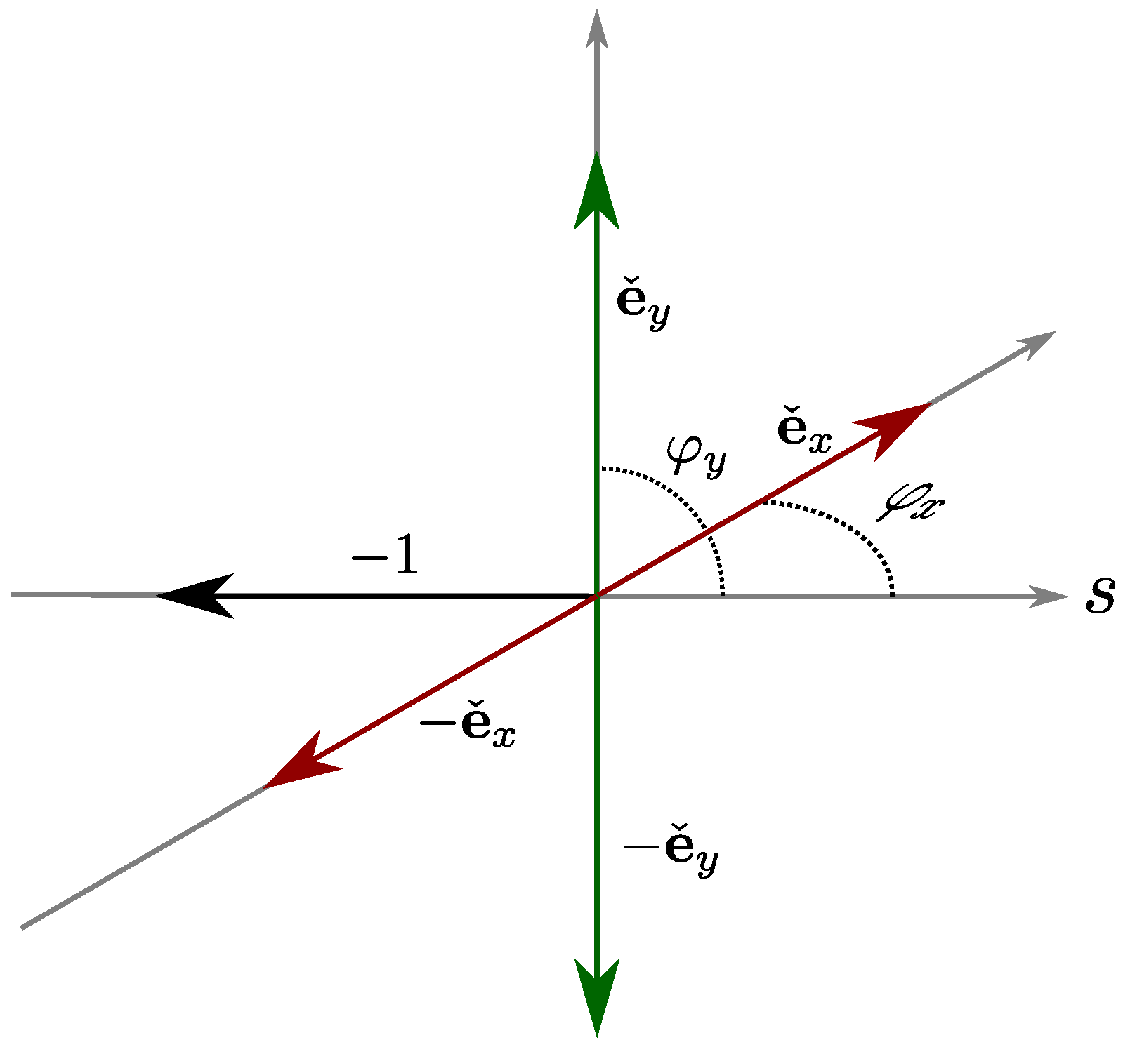
The square roots of minus one in the scator set are the familiar imaginary units of complex algebra, but there is now an imaginary unit for each hypercomplex axis direction. These roots are illustrated in Figure 1. The scalar component and the two director components have been depicted in orthogonal directions. The director coefficients in multiplicative variables ${\phi }_x$ and ${\phi }_y$ are geometrically represented by the angle between the scalar (real) axis and the corresponding hyperimaginary director axis. The product of the roots ${\check{\mathbf{e}}}_x{\check{\mathbf{e}}}_x$ involves a $\frac{\pi }{2}$ rotation in the $s,{\check{\mathbf{e}}}_x$ plane, whereas the product $\left(-{\check{\mathbf{e}}}_x\right)\left(-{\check{\mathbf{e}}}_x\right)$ produces a $\frac{3\pi }{2}$ rotation. An analogous behaviour occurs in the $s,{\check{\mathbf{e}}}_y$ plane for the $\pm {\check{\mathbf{e}}}_y$ roots. These two cases exhaust the possibilities in ${\mathbb{S}}^{1+2}$.

Spurious roots of -1: However, in ${\mathbb{S}}^{1+3}$, minus one can be written as $cos\left(\pi \right)cos\left(\pi \right)$$cos\left(\pi \right)+cos\left(\pi \right)cos\left(\pi \right)sin\left(\pi \right){\check{\mathbf{e}}}_x+cos\left(\pi \right)cos\left(\pi \right)sin\left(\pi \right){\check{\mathbf{e}}}_y$. The solution from (5) is zero:

$$\begin{array}{c}{\stackrel{0}{\zeta }}_{r_x{r}_y{r}_z}\left(1;\pi ,\pi ,\pi \right)={\left(-\stackrel{0}{1}\right)}^{\frac{1}{2}}=cos\left(\frac{\pi }{2}+\pi r_x\right)cos\left(\frac{\pi }{2}+\pi r_y\right)cos\left(\frac{\pi }{2}+\pi r_z\right)\hfill \\ +cos\left(\pi r_y\right)cos\left(\frac{\pi }{2}+\pi r_z\right)sin\left(\frac{\pi }{2}+\pi r_x\right){\check{\mathbf{e}}}_x+cos\left(\frac{\pi }{2}+\pi r_x\right)cos\left(\frac{\pi }{2}+\pi r_z\right)sin\left(\frac{\pi }{2}+\pi r_y\right){\check{\mathbf{e}}}_y\\ \hfill +cos\left(\frac{\pi }{2}+\pi r_x\right)cos\left(\frac{\pi }{2}+\pi r_y\right)sin\left(\frac{\pi }{2}+\pi r_z\right){\check{\mathbf{e}}}_z=0.\end{array}$$

In terms of the components factors, this solution is

$$\begin{array}{c}\left(cos\left(\frac{\pi }{2}+\pi r_x\right)+sin\left(\frac{\pi }{2}+\pi r_x\right){\check{\mathbf{e}}}_x\right)\left(cos\left(\frac{\pi }{2}+\pi r_y\right)+sin\left(\frac{\pi }{2}+\pi r_y\right){\check{\mathbf{e}}}_y\right)\hfill \\ \hspace{1em}\hspace{1em}\hspace{1em}\hspace{1em}\hspace{1em}\hspace{1em}\hspace{1em}\hspace{1em}\hspace{1em}\hspace{1em}\left(cos\left(\frac{\pi }{2}+\pi r_z\right)+sin\left(\frac{\pi }{2}+\pi r_z\right){\check{\mathbf{e}}}_z\right)=\left(\pm {\check{\mathbf{e}}}_x\right)\left(\pm {\check{\mathbf{e}}}_y\right)\left(\pm {\check{\mathbf{e}}}_z\right).\hfill \end{array}$$

Evaluation of the square is ${\stackrel{0}{\zeta }}_{r_x{r}_y{r}_z}^2\left(1;\pi ,\pi ,\pi \right)={\left[\left(\pm {\check{\mathbf{e}}}_x\right)\left(\pm {\check{\mathbf{e}}}_y\right)\left(\pm {\check{\mathbf{e}}}_z\right)\right]}^2$. Depending on the association, this expression is zero or minus one. Thus, this non-associative solution is a spurious root. Notice that the minus one association, $\left[\left(\pm {\check{\mathbf{e}}}_x\right)\left(\pm {\check{\mathbf{e}}}_x\right)\right]\left[\left(\pm {\check{\mathbf{e}}}_y\right)\left(\pm {\check{\mathbf{e}}}_y\right)\right]\left[\left(\pm {\check{\mathbf{e}}}_z\right)\left(\pm {\check{\mathbf{e}}}_z\right)\right]=-1$, again cannot be written as the product of two equal expressions.

Square roots can be readily generalized to $1+n$ dimensions. Consider four subsets of ${\mathbb{S}}^{1+n}$: (i) the set of positive real numbers ${\mathbb{S}}_{+}^{1+0}$, (ii) the set of negative real numbers ${\mathbb{S}}_{-}^{1+0}$, (iii) the set of scators with at least one non vanishing director component ${\mathbb{S}}^{1+n}\setminus {\mathbb{S}}^{1+0}$, and (iv) zero.

(i) For elements in the $\stackrel{o}{\phi }\in {\mathbb{S}}_{+}^{1+0}$ subset, there are only two different square roots. In additive variables, given a scator with non-zero positive scalar and zero director components, $\stackrel{o}{\phi }=f_0+{\sum }_{j=1}^{n}0{\check{\mathbf{e}}}_j$, the two square roots are $\sqrt{\stackrel{o}{\phi }}=\pm \sqrt{f_0}$. In multiplicative variables, given a scator with a non-zero magnitude ${\phi }_0$ and director components equal to zero or a multiple of $2\pi$, the square root is $\sqrt{\stackrel{o}{\phi }}=\sqrt{{\phi }_0}{\prod }_{k=1}^{n}cos\left(0+\pi r_k\right)+\sqrt{{\phi }_0}{\sum }_{j=1}^n{\prod }_{k\ne j}^{n}cos\left(0+\pi r_k\right)sin\left(0+\pi r_j\right){\check{\mathbf{e}}}_j$, and the two different square roots are $\sqrt{\stackrel{o}{\phi }}=\pm \sqrt{{\phi }_0}$, where the ±sign depends on whether there is an even or odd number of director component arguments equal to $\pi$. The geometrical interpretation of the roots in this case is the familiar cyclotomic division. For example, the root lying on the negative scalar axis makes a $\pi$ angle with respect to the positive scalar (or real) axis. The product of the scator root with itself doubles the angle, thereby mapping $-1$ onto 1, as in the complex case.

(ii) For elements in the $\stackrel{o}{\phi }\in {\mathbb{S}}_{-}^{1+0}\subset {\mathbb{S}}^{1+n}$ subset, there exist $2n$ square roots. In additive variables, elements with negative additive scalar and zero director components are considered, $\stackrel{o}{\phi }=-f_0+{\sum }_{j=1}^{n}0{\check{\mathbf{e}}}_j$. In multiplicative variables, all except one of the director components are zero (mod $2\pi$). If, for example, the ${\check{\mathbf{e}}}_l$ direction has a $\pi$ argument, then

$$\begin{array}{c}\stackrel{o}{\phi }={\phi }_{0}cos\left(\pi +2\pi r_l\right)\prod _{k\ne l}^{n}cos\left(2\pi r_k\right)\hfill \\ \hspace{1em}\hspace{1em}\hspace{1em}\hspace{1em}\hspace{1em}\hspace{1em}+{\phi }_0\sum _{j\ne l}^n\prod _{k\ne j}^{n}cos\left(2\pi r_k\right)sin\left(2\pi r_j\right){\check{\mathbf{e}}}_j+{\phi }_0\prod _{k\ne l}^{n}cos\left(2\pi r_k\right)sin\left(\pi +2\pi r_l\right){\check{\mathbf{e}}}_l.\hfill \end{array}$$

The square roots from the Victoria Equation (5) are

$$\begin{array}{c}\sqrt{\stackrel{o}{\phi }}=\sqrt{{\phi }_0}cos\left(\frac{\pi }{2}+\pi r_l\right)\prod _{k\ne l}^{n}cos\left(\pi r_k\right)\hfill \\ \hspace{1em}\hspace{1em}\hspace{1em}\hspace{1em}\hspace{1em}\hspace{1em}+\sqrt{{\phi }_0}\sum _{j\ne l}^n\prod _{k\ne j}^{n}cos\left(\pi r_k\right)sin\left(\pi r_j\right){\check{\mathbf{e}}}_j+\sqrt{{\phi }_0}\prod _{k\ne l}^{n}cos\left(\pi r_k\right)sin\left(\frac{\pi }{2}+\pi r_l\right){\check{\mathbf{e}}}_l,\hfill \end{array}$$

where the only non vanishing term is

$$\sqrt{\stackrel{o}{\phi }}=\sqrt{{\phi }_0}\prod _{k\ne l}^{n}cos\left(\pi r_k\right)sin\left(\frac{\pi }{2}+\pi r_l\right){\check{\mathbf{e}}}_l.$$

There are thus two roots, $\pm \sqrt{\left|f_0\right|}{\check{\mathbf{e}}}_j=\pm \sqrt{{\phi }_0}{\check{\mathbf{e}}}_j$, for each j from 1 to n. In a geometrical representation, the root lying on the ${\check{\mathbf{e}}}_l$ axis makes a $\pm \frac{\pi }{2}$ angle with respect to the scalar (or real) axis. The product of the scator root with itself doubles the angle, thereby mapping the imaginary unit onto the negative scalar axis. However, there are now n hyper imaginary axes, each of them mapping positive or negative numbers on the $\pm {\check{\mathbf{e}}}_j$ line onto the negative scalar axis.

(iii) For elements $\stackrel{o}{\phi }\in {\mathbb{S}}^{1+n}\setminus {\mathbb{S}}^{1+0}$, there are only two different square roots in the additive representation, because the possible $\pi$ phase differences in the $r_j$ coefficients can only introduce an overall $-1$ factor, i.e., $cos\left(\frac{{\phi }_j}{2}+\pi r_j\right)={\left(-1\right)}^{r_j}cos\left(\frac{{\phi }_j}{2}\right)$, and $sin\left(\frac{{\phi }_j}{2}+\pi r_j\right)={\left(-1\right)}^{r_j}sin\left(\frac{{\phi }_j}{2}\right)$. The two square roots are

$$\begin{array}{c}{\left({\phi }_0\prod _{k=1}^{n}cos\left({\phi }_k\right)+\sum _{j=1}^n{\phi }_0\prod _{k\ne j}^{n}cos\left({\phi }_k\right)sin\left({\phi }_j\right){\check{\mathbf{e}}}_j\right)}^{\frac{1}{2}},\hfill \\ \hspace{1em}\hspace{1em}\hspace{1em}\hspace{1em}\hspace{1em}\hspace{1em}=\left(\prod _{j=1}^n{\left(-1\right)}^{r_j}\right){\phi }_0^{\frac{1}{2}}\left(\prod _{k=1}^{n}cos\left(\frac{{\phi }_j}{2}\right)+\sum _{j=1}^n\prod _{k\ne j}^{n}cos\left(\frac{{\phi }_j}{2}\right)sin\left(\frac{{\phi }_j}{2}\right){\check{\mathbf{e}}}_j\right).\hfill \end{array}$$

(17)

(iv) The square of zero is ${\stackrel{o}{0}}^2=\stackrel{o}{0}$; hence, the square root of zero is zero. This is the unique element with only one square root.

The square roots of a scator number $\stackrel{o}{\phi }$ are solutions to the polynomial equation ${\stackrel{o}{\zeta }}^2-\stackrel{o}{\phi }=0$. In particular, square roots of one satisfy the polynomial ${\stackrel{o}{\zeta }}^2-1=0$. The second order polynomial with a non-zero linear term is ${\stackrel{o}{\zeta }}^2+b\stackrel{o}{\zeta }-1=0$, where b is a real coefficient. Surprisingly, this second order polynomial has additional roots that are not present if $b=0$. In ${\mathbb{S}}^{1+2}$, depending on the value of the real number b, the polynomial ${\stackrel{o}{\zeta }}^2+b\stackrel{o}{\zeta }-1=0$ has two, six, or eight scator roots [13].

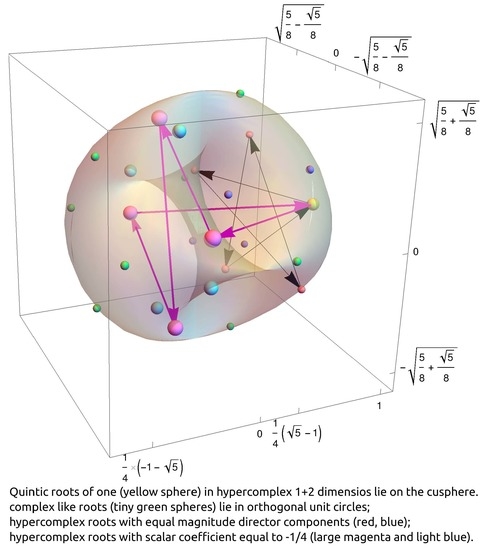
4. Cube Roots of 1

The cube roots of $\stackrel{o}{1}$ in ${\mathbb{S}}^{1+2}$ are given by the Victoria equation for $q=3$ and $n=2$:

$$\begin{array}{c}{\left(cos\left(0\right)cos\left(0\right)+cos\left(0\right)sin\left(0\right){\check{\mathbf{e}}}_x+cos\left(0\right)sin\left(0\right){\check{\mathbf{e}}}_y\right)}^{\frac{1}{3}}=\hfill \\ cos\left(\frac{2\pi r_x}{3}\right)cos\left(\frac{2\pi r_y}{3}\right)+cos\left(\frac{2\pi r_y}{3}\right)sin\left(\frac{2\pi r_x}{3}\right){\check{\mathbf{e}}}_x+cos\left(\frac{2\pi r_x}{3}\right)sin\left(\frac{2\pi r_y}{3}\right){\check{\mathbf{e}}}_y.\hfill \end{array}$$

(18)

Labelling the roots ${\stackrel{o}{\zeta }}_{r_x{r}_y}$, the $q^n=3^2$ values are shown in

Table 1. Cube roots of $\stackrel{o}{1}\in {\mathbb{S}}^{1+2}$ in the additive representation. The second row and second column are the usual cyclotomic complex roots repeated in orthogonal planes. The remaining hypercomplex four roots have no complex analogue.

	${\mathit{r}}_{\mathit{x}}=0$	${\mathit{r}}_{\mathit{x}}=1$	${\mathit{r}}_{\mathit{x}}=2$
$r_y=0$	${\stackrel{o}{\zeta }}_{00}^3=\stackrel{o}{\phi }=1$	${\stackrel{o}{\zeta }}_{10}=-\frac{1}{2}+\frac{\sqrt{3}}{2}{\check{\mathbf{e}}}_x$	${\stackrel{o}{\zeta }}_{20}=-\frac{1}{2}-\frac{\sqrt{3}}{2}{\check{\mathbf{e}}}_x$
$r_y=1$	${\stackrel{o}{\zeta }}_{01}=-\frac{1}{2}+\frac{\sqrt{3}}{2}{\check{\mathbf{e}}}_y$	${\stackrel{o}{\zeta }}_{11}=\frac{1}{4}-\frac{\sqrt{3}}{4}{\check{\mathbf{e}}}_x-\frac{\sqrt{3}}{4}{\check{\mathbf{e}}}_y$	${\stackrel{o}{\zeta }}_{21}=\frac{1}{4}+\frac{\sqrt{3}}{4}{\check{\mathbf{e}}}_x-\frac{\sqrt{3}}{4}{\check{\mathbf{e}}}_y$
$r_y=2$	${\stackrel{o}{\zeta }}_{02}=-\frac{1}{2}-\frac{\sqrt{3}}{2}{\check{\mathbf{e}}}_y$	${\stackrel{o}{\zeta }}_{12}=\frac{1}{4}-\frac{\sqrt{3}}{4}{\check{\mathbf{e}}}_x+\frac{\sqrt{3}}{4}{\check{\mathbf{e}}}_y$	${\stackrel{o}{\zeta }}_{22}=\frac{1}{4}+\frac{\sqrt{3}}{4}{\check{\mathbf{e}}}_x+\frac{\sqrt{3}}{4}{\check{\mathbf{e}}}_y$

. The roots ${\stackrel{o}{\zeta }}_{r_{x}0}$ and ${\stackrel{o}{\zeta }}_{0r_y}$ are the familiar three cyclotomic complex roots, but there are now two circles, one for each scalar-director mutually orthogonal plane, as depicted in Figure 2. They account for four roots, in addition, of course, to $\stackrel{o}{1}$. The remaining four hypercomplex roots have non-zero director coefficients with equal magnitude $\left|x\right|=\left|y\right|=\frac{\sqrt{3}}{4}$ in both director axes. The roots ${\stackrel{o}{\zeta }}_{00}=\stackrel{o}{1}$, ${\stackrel{o}{\zeta }}_{11}=\frac{1}{4}-\frac{\sqrt{3}}{4}{\check{\mathbf{e}}}_x-\frac{\sqrt{3}}{4}{\check{\mathbf{e}}}_y,$ and ${\stackrel{o}{\zeta }}_{22}=\frac{1}{4}+\frac{\sqrt{3}}{4}{\check{\mathbf{e}}}_x+\frac{\sqrt{3}}{4}{\check{\mathbf{e}}}_y$ form a group since ${\stackrel{o}{\zeta }}_{11}^2={\stackrel{o}{\zeta }}_{22}$ and ${\stackrel{o}{\zeta }}_{11}^3={\stackrel{o}{\zeta }}_{22}{\stackrel{o}{\zeta }}_{11}=\stackrel{o}{1}$. These three points lie on the parametric curve

$$cos\left(t\right)cos\left(t\right)+cos\left(t\right)sin\left(t\right){\check{\mathbf{e}}}_x+cos\left(t\right)sin\left(t\right){\check{\mathbf{e}}}_y,$$

(19)

depicted in red in Figure 2. The two-dimensional surface embedded in three-dimensional space of scators $s+x{\check{\mathbf{e}}}_x+y{\check{\mathbf{e}}}_y$ with unit magnitude is

$$1=s^2\left(1+\frac{x^2}{s^2}\right)\left(1+\frac{y^2}{s^2}\right),$$

(20)

where zero $\left(0;0,0\right)$ is clearly excluded. This surface is known as a cusphere [11]. The product of the magnitudes is equal to the magnitude of the products since associativity is satisfied, so that all roots have a magnitude equal to one. Therefore, all the roots lie on the isometric surface as shown in Figure 2.

Perform a Euclidean 45° rotation of the cusphere about the s axis to bring the hypercomplex roots onto the $s,{\check{\mathbf{e}}}_x$ and $s,{\check{\mathbf{e}}}_y$ planes:

$$s^2=\left(s^2+{\left(\frac{1}{\sqrt{2}}x+\frac{1}{\sqrt{2}}y\right)}^2\right)\left(s^2+{\left(-\frac{1}{\sqrt{2}}x+\frac{1}{\sqrt{2}}y\right)}^2\right).$$

At the $y=0$ plane,

$$s=s^2+\frac{x^2}{2},$$

where the positive sign was taken since the magnitude is defined by the positive square root of (20). Shift s by $\frac{1}{2}$ in the negative s direction, $s\to s+\frac{1}{2}$, to obtain $1=4s^2+2x^2,$ that is, an equation of an ellipse with semi-axes $\frac{1}{2}$ and $\frac{1}{\sqrt{2}}$. The unshifted ellipse is centred at $s=\frac{1}{2}$ on the scalar axis. This ellipse and its counterpart, obtained at the $x=0$ plane in the rotated cusphere, are drawn in red in Figure 2. The roots ${\stackrel{o}{\zeta }}_{00}$, ${\stackrel{o}{\zeta }}_{12}$, and ${\stackrel{o}{\zeta }}_{21}$, which lie on the ellipse at $-45{}^{\circ }$ with respect to the ${\check{\mathbf{e}}}_x,{\check{\mathbf{e}}}_y$ axes, also form a group, ${\stackrel{o}{\zeta }}_{12}^2={\stackrel{o}{\zeta }}_{21}$, ${\stackrel{o}{\zeta }}_{21}^2={\stackrel{o}{\zeta }}_{12}$, and their cubes are equal to ${\stackrel{o}{\zeta }}_{00}=\stackrel{o}{1}$. The parametric curve for this ellipse is $cos\left(t\right)cos\left(t\right)+cos\left(t\right)sin\left(t\right){\check{\mathbf{e}}}_x-cos\left(t\right)sin\left(t\right){\check{\mathbf{e}}}_y$. The 45° Euclidean rotation maps the hypercomplex roots to $\frac{1}{4}\pm \frac{\sqrt{6}}{4}{\check{\mathbf{e}}}_x$ and $\frac{1}{4}\pm \frac{\sqrt{6}}{4}{\check{\mathbf{e}}}_y$, but these roots no longer have unit scator magnitude. The Euclidean rotation is an auxiliary procedure to exhibit the types of curves that are being obtained. However, the rotated figures must be treated with much care because a Euclidean rotation does not preserve the scator metric, as may be readily seen from (20).

The projection of the parametric curve (19) in the $s,{\check{\mathbf{e}}}_x$ plane is $cos\left(t\right)cos\left(t\right)+cos\left(t\right)$$sin\left(t\right){\check{\mathbf{e}}}_x$ = $\frac{1}{2}+\frac{1}{2}cos\left(2t\right)+\frac{1}{2}sin\left(2t\right){\check{\mathbf{e}}}_x$. The projections of the unrotated ellipses onto the $s,{\check{\mathbf{e}}}_x$ and $s,{\check{\mathbf{e}}}_y$ planes are thus circles of radius $\frac{1}{4}$, centred at $s=\frac{1}{2}$. The parameter is doubled, so that a 0 to $\pi$ span describes the complete curve. The hypercomplex root ${\stackrel{o}{\zeta }}_{22}=\frac{1}{4}+\frac{\sqrt{3}}{4}{\check{\mathbf{e}}}_x+\frac{\sqrt{3}}{4}{\check{\mathbf{e}}}_y$ makes an angle ${\phi }_x=arctan\sqrt{3}=\frac{\pi }{3}$, measured from the origin (${\stackrel{o}{\zeta }}_{21}=\frac{1}{4}+\frac{\sqrt{3}}{4}{\check{\mathbf{e}}}_x-\frac{\sqrt{3}}{4}{\check{\mathbf{e}}}_y$ is superimposed in this projection). However, if the reference point is $\left(\frac{1}{2};0,0\right)$, this root makes an angle of $\frac{2\pi }{3}$ with respect to the scalar axis, as shown in Figure 3. The ${\stackrel{o}{\zeta }}_{11}=\frac{1}{4}-\frac{\sqrt{3}}{4}{\check{\mathbf{e}}}_x-\frac{\sqrt{3}}{4}{\check{\mathbf{e}}}_y$ root (and its superimposed projection ${\stackrel{o}{\zeta }}_{12}=\frac{1}{4}-\frac{\sqrt{3}}{4}{\check{\mathbf{e}}}_x+\frac{\sqrt{3}}{4}{\check{\mathbf{e}}}_y$) exhibit an analogous behaviour. The parametric curve $\frac{1}{2}+\frac{1}{2}cos\left(2t\right)+\frac{1}{2}sin\left(2t\right){\check{\mathbf{e}}}_x$, drawn in red in Figure 3, is therefore trisected by the hypercomplex roots.

There is a $2\pi$ phase increase in each director angle, as the closed curves at 45° with respect to the ${\check{\mathbf{e}}}_x,{\check{\mathbf{e}}}_y$ axes return to an arbitrary departure point. The geometrical descriptions in Figure 2, Figure 3 and Figure 5, as well as in ([6], Figure 3), suggest that the equal director roots or powers go around the point $\stackrel{o}{c}=\frac{1}{2}+0{\check{\mathbf{e}}}_x+0{\check{\mathbf{e}}}_y$. However, $\stackrel{o}{c}$ is not a singularity. For $t=\frac{\pi }{2}$, the parametric curve is equal to $\stackrel{o}{0}$, but this point should not be included in the curve. Recall that zero is not in the cusphere, because the unit magnitude surface cannot include a point that has zero magnitude. Nonetheless, the cusphere points come arbitrarily close to zero. In this sense, the 45° curves come as close as possible to the singularity but jump it, rather than going around it. It is too large a leap to discuss monodromy when many issues, such as giving an unambiguous meaning to ’going around’ in higher dimensional spaces or the topology of the scator space, need to be addressed first. Nonetheless, this part of the discussion aims to show that some of these ideas seem likely to be meaningful in scator algebra.

5. Fourth Roots of 1

Fourth roots of the multiplicative neutral $\stackrel{o}{1}$ are a singular case because spurious nilroots are present from the outset. The 16 possible roots in ${\mathbb{S}}^{1+2}$, obtained from (5),

$$\begin{array}{c}{\left(cos\left(0\right)cos\left(0\right)+cos\left(0\right)sin\left(0\right){\check{\mathbf{e}}}_x+cos\left(0\right)sin\left(0\right){\check{\mathbf{e}}}_y\right)}^{\frac{1}{4}}\hfill \\ \hspace{1em}\hspace{1em}=cos\left(\frac{\pi r_x}{2}\right)cos\left(\frac{\pi r_y}{2}\right)+cos\left(\frac{\pi r_y}{2}\right)sin\left(\frac{\pi r_x}{2}\right){\check{\mathbf{e}}}_x+cos\left(\frac{\pi r_x}{2}\right)sin\left(\frac{\pi r_y}{2}\right){\check{\mathbf{e}}}_y,\hfill \end{array}$$

(21)

are shown in

Table 2. Fourth roots of $\stackrel{o}{1}\in {\mathbb{S}}^{1+2}$ in the additive representation. This set of roots does not satisfy group properties. There are six different fourth roots of one, $\pm 1$, $\pm {\check{\mathbf{e}}}_x$, and $\pm {\check{\mathbf{e}}}_y$. Spurious nilroots (greyed out) are not roots of $\stackrel{o}{1}$ and should be discarded.

	${\mathit{r}}_{\mathit{x}}=0$	${\mathit{r}}_{\mathit{x}}=1$	${\mathit{r}}_{\mathit{x}}=2$	${\mathit{r}}_{\mathit{x}}=3$
$r_y=0$	1	${\check{\mathbf{e}}}_x$	$-1$	$-{\check{\mathbf{e}}}_x$
$r_y=1$	${\check{\mathbf{e}}}_y$	0	$-{\check{\mathbf{e}}}_y$	0
$r_y=2$	$-1$	$-{\check{\mathbf{e}}}_x$	1	${\check{\mathbf{e}}}_x$
$r_y=3$	$-{\check{\mathbf{e}}}_y$	0	${\check{\mathbf{e}}}_y$	0

.

The (four) roots 1 and $-1$ are the square roots doubled period. The $\pm {\check{\mathbf{e}}}_x$ and $\pm {\check{\mathbf{e}}}_y$ roots with $r_y=0$ and $r_x=0$, respectively, correspond to the complex cyclotomic fourth roots, evaluated on the $s,{\check{\mathbf{e}}}_x$ and $s,{\check{\mathbf{e}}}_y$ planes. The $\pm {\check{\mathbf{e}}}_x$ and $\pm {\check{\mathbf{e}}}_y$ hypercomplex roots with $r_x\ne 0$ and $r_y\ne 0$ have minus sign contributions in the products due to the even rs but are otherwise analogous to the previous roots. When $r_x,r_y$ are odd, both director coefficients are odd multiples of $\frac{\pi }{2}$. A zero scator is thus obtained in the additive representation. These four odd $r_x,r_y$ are spurious nilroots (Corollary 2). Recall that lack of associativity arises if the additive scalar component of a product vanishes. In this case, the first warning came from the $\pm {\check{\mathbf{e}}}_x$, (or $\pm {\check{\mathbf{e}}}_y$) roots that square to $-1$, but their cube ${\left(\pm {\check{\mathbf{e}}}_x\right)}^3=\mp {\check{\mathbf{e}}}_x$ has a vanishing scalar. Nonetheless, associativity holds because there is only one non-zero director component in either representation. However, when $r_x,r_y$ are both odd, there are two non-zero multiplicative director components, and the products no longer associate in the additive representation.

The set of all fourth roots of one does not satisfy group properties in the additive representation even if nilroots are dismissed, because products of orthogonal roots are zero and associativity between different unit orthogonal roots is not satisfied, i.e., $\left({\check{\mathbf{e}}}_x{\check{\mathbf{e}}}_x\right)\left({\check{\mathbf{e}}}_y{\check{\mathbf{e}}}_y\right)=1\ne {\check{\mathbf{e}}}_x\left({\check{\mathbf{e}}}_x{\check{\mathbf{e}}}_y\right){\check{\mathbf{e}}}_y=0$. Nonetheless, there are four $Z_4$ and three $Z_2$ cyclic groups and a Klein four group, represented graphically in Figure 4.

In contrast, consider the multiplicative representation where the product satisfies commutative group properties and the exponent distributes over the factors. In ${\mathbb{S}}^{1+2}$, the fourth roots of unity are

$${\stackrel{o}{1}}^{\frac{1}{4}}=exp\left(\frac{\pi }{2}{r}_x{\check{\mathbf{e}}}_x\right)exp\left(\frac{\pi }{2}{r}_y{\check{\mathbf{e}}}_y\right).$$

The 16 possible roots in the multiplicative representation are shown in

Table 3. Fourth roots of $\stackrel{o}{1}\in {\mathbb{S}}^{1+2}$ in the multiplicative representation, where these expressions are irreducible. These roots satisfy Abelian group properties; their proper subgroups are shown in Figure 4.

	${\mathit{r}}_{\mathit{x}}=0$	${\mathit{r}}_{\mathit{x}}=1$	${\mathit{r}}_{\mathit{x}}=2$	${\mathit{r}}_{\mathit{x}}=3$
$r_y=0$	$e^{0{\check{\mathbf{e}}}_x}{e}^{0{\check{\mathbf{e}}}_y}$	$e^{\frac{\pi }{2}{\check{\mathbf{e}}}_x}{e}^{0{\check{\mathbf{e}}}_y}$	$e^{\pi {\check{\mathbf{e}}}_x}{e}^{0{\check{\mathbf{e}}}_y}$	$e^{\frac{3\pi }{2}{\check{\mathbf{e}}}_x}{e}^{0{\check{\mathbf{e}}}_y}$
$r_y=1$	$e^{0{\check{\mathbf{e}}}_x}{e}^{\frac{\pi }{2}{\check{\mathbf{e}}}_y}$	$e^{\frac{\pi }{2}{\check{\mathbf{e}}}_x}{e}^{\frac{\pi }{2}{\check{\mathbf{e}}}_y}$	$e^{\pi {\check{\mathbf{e}}}_x}{e}^{\frac{\pi }{2}{\check{\mathbf{e}}}_y}$	$e^{\frac{3\pi }{2}{\check{\mathbf{e}}}_x}{e}^{\frac{\pi }{2}{\check{\mathbf{e}}}_y}$
$r_y=2$	$e^{0{\check{\mathbf{e}}}_x}{e}^{\pi {\check{\mathbf{e}}}_y}$	$e^{\frac{\pi }{2}{\check{\mathbf{e}}}_x}{e}^{\pi {\check{\mathbf{e}}}_y}$	$e^{\pi {\check{\mathbf{e}}}_x}{e}^{\pi {\check{\mathbf{e}}}_y}$	$e^{\frac{3\pi }{2}{\check{\mathbf{e}}}_x}{e}^{\pi {\check{\mathbf{e}}}_y}$
$r_y=3$	$e^{0{\check{\mathbf{e}}}_x}{e}^{\frac{3\pi }{2}{\check{\mathbf{e}}}_y}$	$e^{\frac{\pi }{2}{\check{\mathbf{e}}}_x}{e}^{\frac{3\pi }{2}{\check{\mathbf{e}}}_y}$	$e^{\pi {\check{\mathbf{e}}}_x}{e}^{\frac{3\pi }{2}{\check{\mathbf{e}}}_y}$	$e^{\frac{3\pi }{2}{\check{\mathbf{e}}}_x}{e}^{\frac{3\pi }{2}{\check{\mathbf{e}}}_y}$

. These 16 elements satisfy Abelian group properties. Its proper subgroups are illustrated in Figure 4.

Remark 1.

In the multiplicative representation, the product ${\varphi }_0{\prod }_{j=1}^{n}exp\left({\phi }_j{\check{\mathbf{e}}}_j\right)$ is irreducible ([6], Definition 2), that is, it cannot be further simplified in this representation since the product has already been performed by having evaluated the sum of arguments. In particular, the multiplicative representation of a scator with multiplicative variables ${\varphi }_0=1,{\phi }_j=\pi /2$ is $\stackrel{o}{\phi }={\prod }_{j=1}^{n}exp\left(\frac{\pi }{2}{\check{\mathbf{e}}}_j\right)$, and its magnitude is 1.

The power series of the $\stackrel{o}{\mathrm{c}}\exp$ function is actually the additive representation of this function together with the series expansion of the trigonometric functions. If no reference is made to the power series of the $\stackrel{o}{\mathrm{c}}\exp$ function, as in the previous remark, the question of course arises as to the meaning of this function. The complex exponential can be characterized in several other ways; two of these characterizations have been shown to be also true for the $\stackrel{o}{\mathrm{c}}\exp$ function in ${\mathbb{S}}^{1+n}$: (i) the components exponential function $\stackrel{o}{\mathrm{c}}\exp :{\mathbb{R}}^{1+n}\to {\mathbb{S}}^{1+n}$ is the scator holomorphic function $\stackrel{o}{f}$ of the scator variable $\stackrel{o}{\zeta }$, solution to the differential equation [11]

$$\frac{d\stackrel{o}{f}\left(\stackrel{o}{\zeta }\right)}{d\stackrel{o}{\zeta }}=\stackrel{o}{f}\left(\stackrel{o}{\zeta }\right),$$

$\stackrel{o}{f}\left(\stackrel{o}{\zeta }\right)=\stackrel{o}{\mathrm{c}}\exp \left(\stackrel{o}{\zeta }\right)$, where $\stackrel{o}{\mathrm{c}}\exp \left(\stackrel{o}{0}\right)=\stackrel{o}{1}$. (ii) The components exponential function maps scator addition onto scator multiplication ([6], Lemma 2.1), $\stackrel{o}{\mathrm{c}}\exp \left(\stackrel{o}{\alpha }+\stackrel{o}{\beta }\right)=\stackrel{o}{\mathrm{c}}\exp \left(\stackrel{o}{\alpha }\right)\stackrel{o}{\mathrm{c}}\exp \left(\stackrel{o}{\beta }\right)$. Therefore, the components exponential function makes sense even if its series representation is not invoked. However, the equivalence between these characterizations in ${\mathbb{S}}^{1+n}$ has not been established.

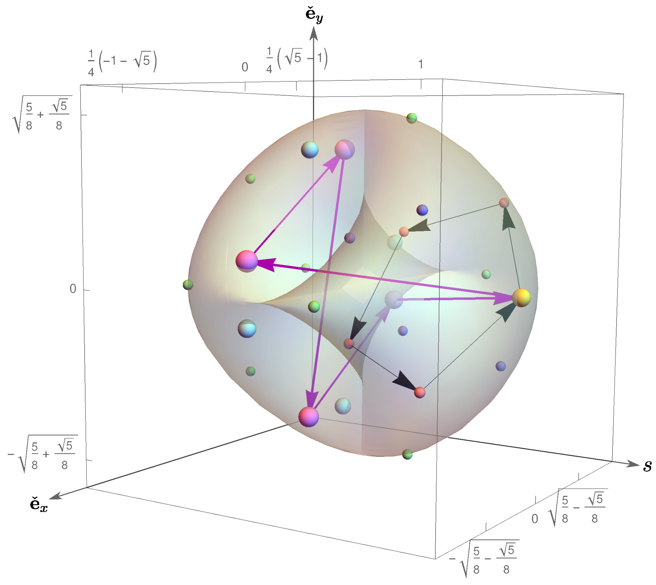
6. Fifth Roots of 1

The Victoria equation for the fifth root of $\stackrel{0}{1}$ in ${\mathbb{S}}^{1+2}$ is

$$\begin{array}{c}{\left(cos\left(0\right)cos\left(0\right)+cos\left(0\right)sin\left(0\right){\check{\mathbf{e}}}_x+cos\left(0\right)sin\left(0\right){\check{\mathbf{e}}}_y\right)}^{\frac{1}{5}}\hfill \\ \hfill =cos\left(\frac{2\pi r_x}{5}\right)cos\left(\frac{2\pi r_y}{5}\right)+cos\left(\frac{2\pi r_y}{5}\right)sin\left(\frac{2\pi r_x}{5}\right){\check{\mathbf{e}}}_x+cos\left(\frac{2\pi r_x}{5}\right)sin\left(\frac{2\pi r_y}{5}\right){\check{\mathbf{e}}}_y.\end{array}$$

(22)

There are $5^2$ possible roots, grouped into six groups with five elements ($6\times 4+1$), all of them sharing, of course, the neutral element, $\stackrel{o}{1}={\stackrel{o}{\zeta }}_{00}$. The roots, labelled ${\stackrel{o}{\zeta }}_{r_x{r}_y},$ with $r_x,r_y$ from 0 to 4, are summarized in

Table 4. Fifth roots of $\stackrel{o}{1}$. The roots are grouped in six cyclic sets. Two cyclotomic-like groups, the two diagonals in the table, correspond to two groups of roots with director equal magnitudes. The last two groups coloured in magenta and teal lie on the $s=-\frac{1}{4}$ plane. However, since $\stackrel{o}{1}={\stackrel{o}{\zeta }}_{00}$ is included in all groups, these last two groups do not lie on a plane.

	${\mathit{r}}_{\mathit{x}}=0$	${\mathit{r}}_{\mathit{x}}=1$	${\mathit{r}}_{\mathit{x}}=2$	${\mathit{r}}_{\mathit{x}}=3$	${\mathit{r}}_{\mathit{x}}=4$
$r_y=0$	$\stackrel{0}{1}={\stackrel{o}{\zeta }}_{00}$	cyclotomic $s,{\check{\mathbf{e}}}_x$
$r_y=1$	cyclotomic $s,{\check{\mathbf{e}}}_y$	${\stackrel{o}{\zeta }}_{11}$	${\stackrel{o}{\zeta }}_{21}$	${\stackrel{o}{\zeta }}_{31}$	${\stackrel{o}{\zeta }}_{41}$
$r_y=2$		${\stackrel{o}{\zeta }}_{12}$	${\stackrel{o}{\zeta }}_{22}$	${\stackrel{o}{\zeta }}_{32}$	${\stackrel{o}{\zeta }}_{42}$
$r_y=3$		${\stackrel{o}{\zeta }}_{13}$	${\stackrel{o}{\zeta }}_{23}$	${\stackrel{o}{\zeta }}_{33}$	${\stackrel{o}{\zeta }}_{43}$
$r_y=4$		${\stackrel{o}{\zeta }}_{14}$	${\stackrel{o}{\zeta }}_{24}$	${\stackrel{o}{\zeta }}_{34}$	${\stackrel{o}{\zeta }}_{44}$

. Two groups, ${\stackrel{o}{\zeta }}_{r_{x}0}$ and ${\stackrel{o}{\zeta }}_{0r_y}$, correspond to the complex cyclotomic fifth roots, evaluated on the $s,{\check{\mathbf{e}}}_x$ and $s,{\check{\mathbf{e}}}_y$ planes. Two other groups correspond to hypercomplex roots with equal magnitude director coefficients that lie on the $\pm 45{}^{\circ }$ planes with respect to the ${\check{\mathbf{e}}}_x,{\check{\mathbf{e}}}_y$ axes. These roots have positive s values, $\frac{1}{4}\left(\sqrt{5}\pm 1\right)$. The group of roots ${\stackrel{o}{\zeta }}_{00}$, ${\stackrel{o}{\zeta }}_{11}$, ${\stackrel{o}{\zeta }}_{22}$, ${\stackrel{o}{\zeta }}_{33}$, and ${\stackrel{o}{\zeta }}_{44}$ has director components with equal signs, both positive or both negative. These roots are shown in red in Figure 5, joined by a pentagon with black arrows. The group ${\stackrel{o}{\zeta }}_{00}$, ${\stackrel{o}{\zeta }}_{14}$, ${\stackrel{o}{\zeta }}_{23}$, ${\stackrel{o}{\zeta }}_{32}$, and ${\stackrel{o}{\zeta }}_{41}$ has director components with equal magnitudes but opposite signs (purple in Figure 5). They exhibit the same structure of the iso-director magnitude groups of the cubic roots. There are now another two sets with a structure that is not present in roots of unity with $q<5$, ${\stackrel{o}{\zeta }}_{12}$, ${\stackrel{o}{\zeta }}_{24}$, ${\stackrel{o}{\zeta }}_{31}$, ${\stackrel{o}{\zeta }}_{43}$, ${\stackrel{o}{\zeta }}_{21}$, ${\stackrel{o}{\zeta }}_{42}$, ${\stackrel{o}{\zeta }}_{13}$, and ${\stackrel{o}{\zeta }}_{34}$. All eight roots, depicted in magenta and light blue in Figure 5, have the same negative additive scalar coefficient, $s=\frac{1}{4}\left(-1+\sqrt{5}\right)\frac{1}{4}\left(-1-\sqrt{5}\right)=-\frac{1}{4}$. These eight roots lie on the $s=-\frac{1}{4}$ plane, but $\stackrel{o}{1}={\stackrel{o}{\zeta }}_{00}$ does not lie in this plane. Therefore, the five elements of these two groups no longer lie on a plane as in previous cases. The $Z_{5^2}$ proper Abelian subgroups of these roots are depicted in Figure 6.

7. qth Roots of 1

A scator $\stackrel{o}{\phi }\in {\mathbb{S}}^{1+n}$ raised to the power $\frac{1}{q}$ has $q^n$ possible roots. The roots are obtained from the Victoria root Theorem 2 by evaluation of each of the $r_j$s, from 0 to q, and for j, from 1 to n. In the multiplicative representation, the roots are obtained from Theorem 1. Label the roots for identification with subindices $r_1$ to $r_n$, ${\stackrel{o}{\zeta }}_{r_1{r}_2\cdots r_n}^q=\stackrel{o}{\phi }$.

The roots of unity, provided that associativity of the factors is ensured, can be grouped in cyclic sets that satisfy Abelian group properties with q elements in each set. $q-1$ elements with different $r_j$s belong only to one such set, and the element ${\stackrel{o}{\zeta }}_{00}$ is the identity element, common to all groups. The $q^n$ roots are grouped into g sets; thus, $\left(q-1\right)g+1=q^n$, the number of cyclic groups with q elements, is then

$$g=\frac{q^n-1}{q-1}.$$

For example, for scators in $\stackrel{o}{\phi }\in {\mathbb{S}}^{1+2}$, there are two director components; then, $g=q+1$. For scators in $\stackrel{o}{\phi }\in {\mathbb{S}}^{1+3}$, $g=\frac{q^3-1}{q-1}=q^2+q+1$, there are, in particular, $3^3$ cube roots that can be grouped into $g=13$ sets. The elements of a group are obtained by evaluation of the p powers of any root in the group except the identity, for p from 0 to $q-1$, modulo q. Examples for q equalling 2, 3, and 5 are shown in Figure 6. For example, let ${\stackrel{o}{\zeta }}_{33}$ be a fifth root of $\stackrel{o}{\phi }\in {\mathbb{S}}^{1+2}$: the square is ${\stackrel{o}{\zeta }}_{33}^2={\stackrel{o}{\zeta }}_{66}={\stackrel{o}{\zeta }}_{11}$, the cube ${\stackrel{o}{\zeta }}_{33}^3={\stackrel{o}{\zeta }}_{99}={\stackrel{o}{\zeta }}_{44}$, the fourth power ${\stackrel{o}{\zeta }}_{33}^4={\stackrel{o}{\zeta }}_{12,12}={\stackrel{o}{\zeta }}_{22}$, and the fifth power ${\stackrel{o}{\zeta }}_{33}^5={\stackrel{o}{\zeta }}_{15,15}={\stackrel{o}{\zeta }}_{00}$. For $\stackrel{o}{\phi }=\stackrel{o}{1}$, this sequence produces a pentagon, similar to the one depicted with black arrows in Figure 5. The sequence ${\stackrel{o}{\zeta }}_{00}$, ${\stackrel{o}{\zeta }}_{11}$, ${\stackrel{o}{\zeta }}_{11}^2={\stackrel{o}{\zeta }}_{22}$, ${\stackrel{o}{\zeta }}_{11}^3={\stackrel{o}{\zeta }}_{33}$, and ${\stackrel{o}{\zeta }}_{11}^4={\stackrel{o}{\zeta }}_{44}$ produces a star-like figure, etc. In the multiplicative representation, this scheme is true for any of the $q\mathrm{th}$ roots of unity, since the product is associative. However, in the additive representation, for even $q\mathrm{th}$ roots of unity, the number of roots is reduced, and the set of all roots for a given q does not satisfy group properties. There are, nonetheless, cyclic group subsets within the sets of even q roots, as shown in Figure 4.

Director Conjugate Roots

The conjugate of a scator leaves the scalar part invariant and changes the sign of the director coefficients, either in the additive or the multiplicative representation. The ${\check{\mathbf{e}}}_j$ conjugate or $j\mathrm{th}$director conjugate${\stackrel{o}{\phi }}^{\ast j}$ of a scator $\stackrel{o}{\phi }$ is defined by the negative of the ${\check{\mathbf{e}}}_j$ director component, while all the remaining components are left unchanged [14]. In the present context, we refer to the ${\check{\mathbf{e}}}_j$ period conjugate when the ${\phi }_j$ coefficient of a director is left unaltered, but the fundamental periodicity $2\pi r_j$ changes sign, $\frac{1}{q}\left({\phi }_j+2\pi r_j\right)\mapsto \frac{1}{q}\left({\phi }_j-2\pi r_j\right)$.

Lemma 2.

If ${\stackrel{o}{\zeta }}_{r_1{r}_2\cdots r_n}$ is a $q\mathrm{th}$ root of $\stackrel{o}{\phi }\in {\mathbb{S}}^{1+n}$, a ${\check{\mathbf{e}}}_l$ period conjugate scator of this root ${\stackrel{o}{\zeta }}_{r_1{r}_2,-r_l,\cdots r_n}$ is also a root for any $r_l$ from 1 to n. There are $2^d$ director period conjugate roots for each ordered set of d non-zero $r_j$ elements,$d\le n$.

Proof. 

Since ${\stackrel{o}{\zeta }}_{r_1{r}_2\cdots r_n}$ is a root, in the multiplicative representation,

$${\stackrel{o}{\zeta }}_{r_1{r}_2\cdots r_n}={\phi }_0^{\frac{1}{q}}\prod _{j=1}^n{e}^{\frac{1}{q}\left({\phi }_j+2\pi r_j\right){\check{\mathbf{e}}}_j},$$

so that

$${\stackrel{o}{\zeta }}_{r_1{r}_2\cdots r_n}^q={\phi }_0\prod _{j=1}^n{e}^{\left({\phi }_j+2\pi r_j\right){\check{\mathbf{e}}}_j}={\phi }_0\prod _{j=1}^n{e}^{{\phi }_j{\check{\mathbf{e}}}_j}=\stackrel{o}{\phi }.$$

Let $r_l$ in the $l\mathrm{th}$ term be modified to $q-r_l$, $exp\left(\frac{1}{q}2\pi \left(q-r_l\right)\right)=exp\left(\frac{1}{q}2\pi \left(-r_l\right)\right)$, so that ${\stackrel{o}{\zeta }}_{r_1{r}_2,q-r_l,\cdots r_n}={\stackrel{o}{\zeta }}_{r_1{r}_2,-r_l,\cdots r_n}$. Evaluate ${\stackrel{o}{\zeta }}_{r_1{r}_2,-r_l,\cdots r_n}$ to the power q using Theorem 1,

$${\stackrel{o}{\zeta }}_{r_1{r}_2,-r_l,\cdots r_n}^q=\prod _{j\ne l}^{n}exp\left(\left({\phi }_j+2\pi r_j\right){\check{\mathbf{e}}}_j\right)exp\left(\left({\phi }_l-2\pi r_l\right){\check{\mathbf{e}}}_l\right),$$

but ${\prod }_{j\ne l}^{n}exp\left(2\pi r_j{\check{\mathbf{e}}}_j\right)exp\left(-2\pi r_l{\check{\mathbf{e}}}_l\right)={\prod }_{j=1}^{n}exp\left(0{\check{\mathbf{e}}}_j\right)=\stackrel{o}{1}$; thus, ${\stackrel{o}{\zeta }}_{r_1{r}_2,-r_l,\cdots r_n}^q=\stackrel{o}{\phi }\stackrel{o}{1}=\stackrel{o}{\phi }$. Therefore, ${\stackrel{o}{\zeta }}_{r_1{r}_2,-r_l,\cdots r_n}$ is also a root. Since any or several $r_j$s can be changed by their negative value independently, given a root ${\stackrel{o}{\zeta }}_{r_1{r}_2\cdots r_n}$, $2^d$ roots are obtained from the evaluation of $\pm r_j$ for the ordered sets of $r_j$s different from zero from 1 to n. For $d=n$,

$${\stackrel{o}{\zeta }}_{\pm r_1\pm r_2\cdots \pm r_n}={\phi }_0^{\frac{1}{q}}\prod _{j=1}^n{e}^{\frac{1}{q}\left({\phi }_j\pm 2\pi r_j\right){\check{\mathbf{e}}}_j};$$

For $d=n-1$, ${\stackrel{o}{\zeta }}_{\pm r_1\pm r_2\cdots \pm r_{n-1},0},{\stackrel{o}{\zeta }}_{\pm r_1\pm r_2\cdots 0,\pm r_n},\cdots {\stackrel{o}{\zeta }}_{0,\pm r_2\cdots \pm r_n}$;

$$⋮$$

For $d=1$, ${\stackrel{o}{\zeta }}_{\pm r_1,0,\cdots ,0},{\stackrel{o}{\zeta }}_{0,\pm r_2,\cdots ,0},{\stackrel{o}{\zeta }}_{0,0,\cdots \pm r_n}.$ □

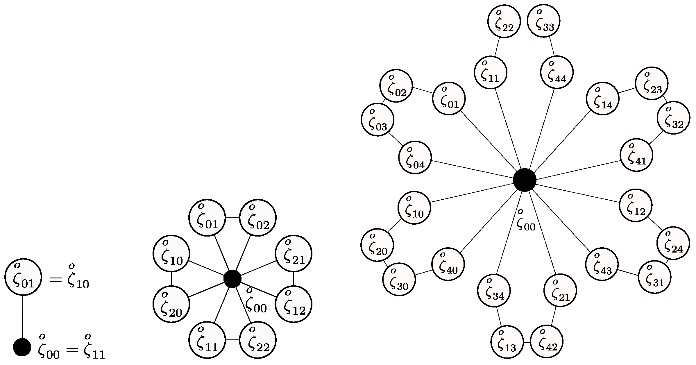
Director conjugation is applied independently to each director component. Only $r_j$s from 1 to $\frac{q-1}{2}$, if q is odd, or $\frac{q}{2}$, if q is even, need to be considered, since $-r_j\mathrm{mod}q$ is equal to $q-r_j$. For roots of $\stackrel{o}{1}$, period director conjugation and director conjugation give the same expressions since ${\phi }_j=0$ for all j. The fifth roots of $\stackrel{o}{1}\in {\mathbb{S}}^{1+2}$ are shown as an example in Figure 7, grouped into nine cyclic sets under director conjugation. These sets clearly do not satisfy group properties, except the trivial single element ${\stackrel{o}{\zeta }}_{00}$ set. Nonetheless, they are cyclic under director conjugation, alternating the conjugation components. For the fifth root, it suffices to consider $\frac{q-1}{2}=2$ non-zero values for $r_j$. For $r_1,r_2\ne 0$, $d=2$, there are four possible combinations of $r_1,r_2$. Each of these four sets have $2^d=2^2$ elements. Take, for instance, the set joined by a horizontal rectangle on the left in Figure 7; the ${\stackrel{o}{\zeta }}_{12}$ element first component conjugation is ${\stackrel{o}{\zeta }}_{12}\to {\stackrel{o}{\zeta }}_{12}^{\ast 1}={\stackrel{o}{\zeta }}_{-12}={\stackrel{o}{\zeta }}_{42}$. The superstar followed by a number notation means the conjugation of the corresponding number position. Negative indices are mod 5 mapped onto positive indices for ease of comparison with Figure 6. Subsequent elements of these sets upon director conjugation are ${\stackrel{o}{\zeta }}_{42}^{\ast 2}\to {\stackrel{o}{\zeta }}_{43}$, ${\stackrel{o}{\zeta }}_{43}^{\ast 1}\to {\stackrel{o}{\zeta }}_{13}$, and ${\stackrel{o}{\zeta }}_{13}^{\ast 2}\to {\stackrel{o}{\zeta }}_{12}$. This set of four elements is also depicted on the right in Figure 7. This clockwise cycle, seen from the positive s axis, becomes an anticlockwise cycle if director conjugation is initiated with the second component. Scator conjugation alternates between diagonal elements in these sets, i.e., ${\stackrel{o}{\zeta }}_{13}^{\ast }\to {\stackrel{o}{\zeta }}_{42}$. Since conjugation is a second order involution, if applied twice, it leaves the element invariant. For $r_1=0,r_2\ne 0$, $d=1$, there are two possible combinations of $r_2$. Each of these two sets have $2^d=2^1$ elements. Another two sets of two elements are obtained for $r_1\ne 0,r_2=0$. The multiplicative identity ${\stackrel{o}{\zeta }}_{00}=\stackrel{o}{1}$ is invariant under conjugation and is the only element in the remaining set.

To summarize the results in this last section, given a $q\mathrm{th}$ root of $\stackrel{o}{1}$ in ${\mathbb{S}}^{1+n}$, its scator conjugate (changing signs to all director components) is also a root. This result is analogous to complex conjugate roots of one in $\mathbb{C}$. Furthermore, the $j\mathrm{th}$ director conjugate of a $q\mathrm{th}$ root (changing sign only to the ${\check{\mathbf{e}}}_j$ director component) is also a root. Since the director conjugate can be subsequently evaluated for any another component, say $l\ne j$, and so on, all director conjugate possibilities of a $q\mathrm{th}$ root are also roots. These roots are a higher dimensional generalization of complex conjugate roots in a $1+n$ scator dimensional space.

8. Conclusions

Integer and rational powers of scators in ${\mathbb{S}}^{1+n}$ have been obtained in the multiplicative (polar) and additive (Cartesian) representations of scators. The Victoria Equation (5) establishes the relationship between the powers of a scator in the additive representation with multiplicative variables and a scator with the concomitant scaling of the trigonometric arguments. The $m\mathrm{th}$ power of a scator $\stackrel{o}{\phi }$ (or root $\stackrel{o}{\zeta }$) is obtained by raising the scator magnitude to the power m and scaling $m{\phi }_j$ for the ${\check{\mathbf{e}}}_j$ director components. The generalization of the De Moivre formula to hypercomplex scator space permits the evaluation of the exponential of a scator in ${\mathbb{S}}^{1+2}$ ([6], Lemma 4). Following a similar procedure, it should be possible to evaluate the exponential of scators with higher dimensions. A geometric interpretation is accomplished if the scalar and hypercomplex axes are drawn in orthogonal directions. For a scator $\stackrel{o}{\phi }={\phi }_0{\prod }_{k=1}^{n}cos{\phi }_k\left(1+tan{\phi }_j{\check{\mathbf{e}}}_j\right)$, each multiplicative variable ${\phi }_j$ represents the angle between the director component ${\check{\mathbf{e}}}_j$ and the scalar axis s. Each hypercomplex component is endowed with a fundamental period. The product of two scators involves a scaling and a rotation in each scalar-hypercomplex plane. If the products are associative in the additive representation, the powers of unit magnitude scators lie on the unit isometric surface, also called a cusphere. The powers of unit scators $\stackrel{o}{\phi }=cos\left({\phi }_x\right)cos\left(\lambda {\phi }_x\right)+cos\left(\lambda {\phi }_x\right)sin\left({\phi }_x\right){\check{\mathbf{e}}}_x+cos\left({\phi }_x\right)sin\left(\lambda {\phi }_x\right){\check{\mathbf{e}}}_y$ belong to points on the $\stackrel{o}{\mathrm{c}}\exp \left(t{\check{\mathbf{e}}}_x+\lambda t{\check{\mathbf{e}}}_y\right)$ parametric curve, where $\stackrel{o}{\mathrm{c}}\exp$ is the components exponential function. The relationship between these objects and modular curves will be undertaken in a forthcoming study. The $q\mathrm{th}$ roots of a scator $\stackrel{o}{\phi }\in {\mathbb{S}}^{1+n}$ are at most $q^n$. The number of roots increases considerably with scator dimension as well as for higher order roots. However, the square roots of unity are $\pm 1$ regardless of the dimension, and there are only $2n$ distinct square roots of $-1$, namely ${\check{\mathbf{e}}}_j{\check{\mathbf{e}}}_j=(-{\check{\mathbf{e}}}_j)(-{\check{\mathbf{e}}}_j)=-1$ for j from 1 to n. The cyclic group structure of square to quintic roots of one has been described, where the action is the scator product. The differences between the set properties in the additive and multiplicative representations for even roots have been studied as well as the origin of spurious roots. The roots have also been classified under the action of scator conjugation.