Article

Mathematical Analysis of a Fractional COVID-19 Model Applied to Wuhan, Spain and Portugal

by
Faïçal Ndaïrou
and
Delfim F. M. Torres
*
Center for Research and Development in Mathematics and Applications (CIDMA), Department of Mathematics, University of Aveiro, 3810-193 Aveiro, Portugal
*
Author to whom correspondence should be addressed.
This research is part of first author’s Ph.D. project, which is carried out at the University of Aveiro under the Doctoral Program in Applied Mathematics of Universities of Minho, Aveiro, and Porto (MAP-PDMA).
Axioms 2021, 10(3), 135; https://doi.org/10.3390/axioms10030135
Submission received: 7 June 2021 / Revised: 22 June 2021 / Accepted: 25 June 2021 / Published: 27 June 2021
(This article belongs to the Special Issue Mathematics of the COVID-19)

Abstract

:
We propose a qualitative analysis of a recent fractional-order COVID-19 model. We start by showing that the model is mathematically and biologically well posed. Then, we give a proof on the global stability of the disease free equilibrium point. Finally, some numerical simulations are performed to ensure stability and convergence of the disease free equilibrium point.

1. Introduction

The study and analysis of the spread of infectious diseases via mathematical models has become an important tool to understand diseases’ epidemiological prototypes, such as prevalence, duration of the epidemic, and its burden on a population. A variety of techniques can be considered in the modeling formulation in order to reflect particularities in the transmission routes of a disease. In general, there exist two major routes:
(i)
direct contact, that is, from infected to non-infected individuals (for instance, through body fluids for Ebola virus disease [1,2,3] or through sexual intercourse for HIV infection [4,5,6] or by non-linearities in the transmission incidence [7,8]);
(ii)
indirect contact, which is due to the presence of carriers in the environment, for example, through mosquitoes and their aquatic phase [9,10,11,12].
These features are fundamental in the transmission process of any disease in leading to specific health status of each individual in the community. Thus, individuals in the community can be classified into disjoints compartments according to their specific health status.
The so-called classical SIR models refer to three epidemiological status (susceptible–infected–recovered) and were firstly introduced by Kermack and McKendrick [13] and constitute the basis foundation of compartmental models. Additionally, some earlier development aiming to introduce demographic factors in compartmental models through birth and death rate were considered by these authors [14,15]. Nowadays, mathematical models are more complex and more realistic by including a large number of health status (see, e.g., [2,4,16] for models with much more epidemiological states). However, in relation to the analysis of these models, one of the challenges is how to establish stability of equilibrium points [17,18,19,20] in order to acquire insights into the dynamics behavior of such models.
Recently, great considerations have been made to models described by fractional differential equations in the field of mathematical epidemiology [21,22,23]. The most essential property of these models is their memory effect [24], which is not appearing in the traditional instantaneous differential equations. This effect is fully captured by flexibility of the order of differentiation for fractional derivatives and can be seen as a hereditary property or a variety on strains and genomes of viruses (as conjectured in [23]), which is useful for epidemic models. In [25], a model for controlling the Coronavirus pandemic 2019 (COVID-19) in India with Caputo–Fabrizio fractional derivatives and the homotopy analysis transform method is investigated. Often, fractional-order models give rise to theoretical models that allow a significant improvement in the fitting of real data, when compared with analogous classical models [26]. However, there are also cases where the fractional-order models do not bring any advantage [27]. In the case of the model under investigation, the fractional-order model has clear advantages to describe the spread of COVID-19 in Galicia, Spain, and Portugal, but does not offer advantages with respect to Wuhan [23]. Precisely, the fractional-order model proposed in [23] describes well the spread of COVID-19 in Spain with order α = 0.85 , in Portugal with order α = 0.75 , and in Wuhan with order α = 1 .
Fractional differential equations can be seen as a sub-field of fractional calculus [28], that is, the mathematical theory that deals with generalization of integrals and derivatives to real or complex order. Furthermore, systems modeled with the help of fractional calculus are non-linear and might display a much more richer dynamical behavior due to properties of order differentiation.
The paper is organized as follows. We start by a preliminary section (Section 2), in which we recall definitions and necessary results of the literature. Then, in Section 3, we present the fractional-order model that we will be studying. Next, in Section 4, we prove the existence and uniqueness of a positive solution. The global stability analysis of the disease free equilibrium point is investigated in Section 5. In Section 6, we present some numerical simulations of the model. We end with Section 7, with our conclusions.

2. Preliminaries on Fractional Calculus

In this section, we begin by presenting the Caputo definition of fractional derivative and then recall some basic properties useful to study the fractional-order model. The reader interested to learn about fractional calculus is referred to [29,30].
The Caputo fractional derivative of order α ( 0 , 1 ) of a function x : [ 0 , + ) R is given by
C D α x ( t ) = 1 Γ ( 1 α ) 0 t ( t s ) α x ( s ) d s ,
where Γ ( 1 α ) = 0 t α exp ( t ) d t is the Euler Gamma function.
Note that the value of the Caputo fractional derivative of the function x at point t involves all the values of x ( s ) for s [ 0 , t ] and, hence, it incorporates the history of x. We also see that C D α x ( t ) tends to x ( t ) as α 1 . The next result is crucial in the study of an initial fractional-order value problem, useful in the proof of our Theorem 1.
Let f : R n R n be a vector function with n > 1 and consider the following fractional-order initial value problem:
C D α X ( t ) = f ( X ) , X ( 0 ) = X 0 , X 0 R n .
Lemma 1
(See [31]). Assume that the vector function f satisfies the following conditions:
  • f ( X ) and f ( X ) X are continuous for all X R n ;
  • f ( X ) ω + λ X for all X R n , where ω and λ are two positive constants.
Then, system (1) has a unique solution.
The following generalized mean value theorem and its consequences are also needed in the proof of Theorem 1.
Lemma 2
(Generalized Mean Value Theorem [31]). Suppose that the functions x ( t ) and C D α x ( t ) are both continuous on [ 0 , b ] . Then,
x ( t ) = x ( 0 ) + 1 Γ ( α ) C D α x ( η ) t α , 0 < η < t , t [ 0 , b ] .
Thus, as consequences of Lemma 2, we have that if C D α x ( t ) > 0 for all t [ 0 , b ] , then the function x is strictly increasing, and if C D α x ( t ) < 0 for all t [ 0 , b ] , then the function x is strictly decreasing.

3. The Considered Fractional-Order COVID-19 Model

In this section, we consider a fractional-order COVID-19 model earlier proposed by Ndaïrou et al. [23]. We shall assume the total population N is constant, along the period under study, and made up with eight sub-population of dynamics transition, as different stages of transmission of the virus to individuals grouped into compartmental classes
S ( t ) + E ( t ) + I ( t ) + P ( t ) + A ( t ) + H ( t ) + R ( t ) + F ( t ) = N
for all t, where S ( t ) denotes the susceptible individuals at time t, E ( t ) the exposed individuals, I ( t ) the symptomatic and infectious individuals, P ( t ) the super-spreaders individuals, A ( t ) the infectious but asymptomatic individuals, H ( t ) the hospitalized individuals, R ( t ) the recovery individuals, and F ( t ) the dead individuals or fatality class. The Caputo fractional-order system that describes the dynamics transmission is given by
C D α S ( t ) = β I ( t ) N S ( t ) l β H ( t ) N S ( t ) β P ( t ) N S ( t ) , C D α E ( t ) = β I ( t ) N S ( t ) + l β H ( t ) N S ( t ) + β P ( t ) N S ( t ) κ E ( t ) , C D α I ( t ) = κ ρ 1 E ( t ) ( γ a + γ i ) I ( t ) δ i I ( t ) , C D α P ( t ) = κ ρ 2 E ( t ) ( γ a + γ i ) P ( t ) δ p P ( t ) , C D α A ( t ) = κ ( 1 ρ 1 ρ 2 ) E ( t ) , C D α H ( t ) = γ a ( I ( t ) + P ( t ) ) γ r H ( t ) δ h H ( t ) , C D α R ( t ) = γ i ( I ( t ) + P ( t ) ) + γ r H ( t ) , C D α F ( t ) = δ i I ( t ) + δ p P ( t ) + δ h H ( t ) .
The expression β I N S + l β H N S + β P N S represents the force of infection of the virus, that is, the transmission term or the effective contact between susceptible individuals (S) and infectious symptomatic individuals (I), super-spreaders individuals (P), and hospitalized ones (H). Here, β quantifies the human-to-human transmission coefficient per unit of time (days) per person, β quantifies a high transmission coefficient due to super-spreaders, l quantifies the relative transmissibility of hospitalized patients. Next, we give a description of the rest of parameters appearing in the model system (2):
  • κ is the rate at which an individual leaves the exposed class by becoming infectious (symptomatic, super-spreaders or asymptomatic);
  • ρ 1 is the proportion of progression from exposed class E to symptomatic infectious class I;
  • ρ 2 is a relative very low rate at which exposed individuals become super-spreaders;
  • 1 ρ 1 ρ 2 is the progression from exposed to asymptomatic class;
  • γ a is the average rate at which symptomatic and super-spreaders individuals become hospitalized;
  • γ i is the recovery rate without being hospitalized;
  • γ r is the recovery rate of hospitalized patients;
  • δ i denotes the disease induced death rates due to infected individuals;
  • δ p denotes the disease induced death rates due to super-spreaders individuals;
  • δ h denotes the disease induced death rates due to hospitalized individuals.
The model was first proposed in [23] for the purpose of fitting real data from Galicia, Spain, and Portugal, but without any mathematical analysis. Here we show that the model is mathematically well posed and it has a unique equilibrium point, which is globally asymptotically stable.

4. Existence and Uniqueness of Positive Solution

First of all, let us rewrite system (2) in a compact form. In doing so, denote
R + 8 = { X R 8 : X 0 }
and let X ( t ) = S ( t ) , E ( t ) , I ( t ) , P ( t ) , A ( t ) , H ( t ) , R ( t ) , F ( t ) T . Then, the system (2) can be rewritten as follows:
C D α X ( t ) = F X ( t ) ,
where
F ( X ) = β I N S l β H N S β P N S β I N S + l β H N S + β P N S κ E κ ρ 1 E ( γ a + γ i ) I δ i I κ ρ 2 E ( γ a + γ i ) P δ p P κ ( 1 ρ 1 ρ 2 ) E γ a ( I + P ) γ r H δ h H γ i ( I + P ) + γ r H δ i I + δ p P + δ h H .
For practical applications reasons, we consider non-negative initial conditions:
S ( 0 ) 0 , E ( 0 ) 0 , I ( 0 ) 0 , P ( 0 ) 0 , A ( 0 ) 0 , H ( 0 ) 0 , R ( 0 ) 0 , F ( 0 ) 0 .
In addition, set
A 1 = 0 0 β β 0 l β 0 0 0 0 β β 0 l β 0 0 0 0 0 0 0 0 0 0 0 0 0 0 0 0 0 0 0 0 0 0 0 0 0 0 0 0 0 0 0 0 0 0 0 0 0 0 0 0 0 0 0 0 0 0 0 0 0 0 , A 2 = 0 0 0 0 0 0 0 0 0 κ 0 0 0 0 0 0 0 κ ρ 1 ϖ i 0 0 0 0 0 0 κ ρ 2 0 ϖ p 0 0 0 0 0 ϖ e 0 0 0 0 0 0 0 0 γ a γ a 0 ϖ h 0 0 0 0 γ i γ i 0 γ r 0 0 0 0 0 δ i δ p 0 δ h 0 ,
where ϖ e = κ ( 1 ρ 1 ρ 2 ) ; ϖ i = γ a + γ i + δ i ; ϖ p = γ a + γ i + δ p ; and ϖ h = γ r + δ h . Thus, we can rewrite the vector function F as
F ( X ) = S N A 1 X + A 2 X .
We are in conditions to state and prove our first result.
Theorem 1
(existence and uniqueness of a non-negative solution). There is a unique solution for the initial value problem given by (2)–(4) and the solution belongs to
Ω = { ( S , E , I , P , A , H , R , F ) R + 8 : S + E + I + P + A + H + R + F N } .
Proof. 
The existence and uniqueness of solution are obtained by application of Theorem 3.1 and Remark 3.2 of [32]. For this purpose, it is easy to check that the vector function is a polynomial, thus continuous and has continuous derivative in Ω . Furthermore, satisfying
F ( X ) A 1 X + A 2 X = A 1 + A 2 X < ϵ + A 1 + A 2 X
for any positive constant ϵ . The proof of non-negativity of solution follows the same spirit as in [33]. By summing up all the 8 equations of system (2), we obtain
C D α S ( t ) + E ( t ) + I ( t ) + P ( t ) + A ( t ) + H ( t ) + R ( t ) + F ( t ) = 0 .
Thus,
0 S ( t ) + E ( t ) + I ( t ) + P ( t ) + A ( t ) + H ( t ) + R ( t ) + F ( t ) S ( 0 ) + E ( 0 ) + I ( 0 ) + P ( 0 ) + A ( 0 ) + H ( 0 ) + R ( 0 ) + F ( 0 ) = N ,
which ends the proof. □

5. Stability Analysis

First of all, note that the model system (2) exhibits a unique steady state which is the disease free equilibrium point (DFE) obtained by setting the right hand side of (2) equal to zero. Precisely, we have
D F E = ( N , 0 , 0 , 0 , 0 , 0 , 0 , 0 ) .
Next, recall that the basic reproduction number for this fractional-order model system is the same as for the classical model investigated in [34] using the next-generation matrix approach [35,36], being given by
R 0 = β ρ 1 ( γ a l + ϖ h ) ϖ i ϖ h + ( β γ a l + β ϖ h ) ρ 2 ϖ p ϖ h .
This can be rewritten in the following manner:
R 0 = β ρ 1 ϖ h ϖ p + β ρ 1 γ a l ϖ p + β ρ 2 ϖ h ϖ i + β ρ 2 γ a l ϖ i ϖ i ϖ p ϖ h ,
which is useful in the below proof of global stability.
Theorem 2
(global stability of the DFE). Let α ( 0 , 1 ) . The disease free equilibrium (DFE) of system (2) is globally asymptotically stable whenever R 0 < 1 .
Proof. 
Consider the following Lyapunov function:
V ( t ) = a 0 E ( t ) + a 1 I ( t ) + a 2 P ( t ) + a 3 H ( t ) ,
where a 0 , a 1 , a 2 , and a 3 are positive constants to be determined. Because the fractional operator C D α is linear, we have that
C D α V ( t ) = a 0 C D α E ( t ) + a 1 C D α I ( t ) + a 2 C D α P ( t ) + a 3 C D α H ( t ) ,
and from (2) it follows that
C D α V ( t ) = a 0 β I N S + l β H N S + β P N S κ E + a 1 κ ρ 1 E ( γ a + γ i ) I δ i I + a 2 κ ρ 2 E ( γ a + γ i ) P δ p P + a 3 γ a ( I + P ) γ r H δ h H .
Next, as S N , we have
C D α V ( t ) a 0 β I + l β H + β P κ E + a 1 κ ρ 1 E ϖ i I + a 2 κ ρ 2 E ϖ p P + a 3 γ a ( I + P ) ϖ h H ,
where ϖ i = γ a + γ i + δ i ; ϖ p = γ a + γ i + δ p ; and ϖ h = γ r + δ h . Rearranging and reducing leads to
C D α V ( t ) ( a 0 β + a 3 γ a a 1 ϖ i ) I + ( a 0 β l a 3 ϖ h ) H + ( a 0 β + a 3 γ a 2 ϖ p ) P + κ ( a 1 ρ 1 + a 2 ρ 2 a 0 ) E .
Now, we choose,
a 0 = ϖ i ϖ p ϖ h ; a 1 = β + β γ a l ϖ h ϖ h ϖ p ; a 2 = β + β γ a l ϖ h ϖ i ϖ h ; a 3 = β l ϖ i ϖ p ,
so that function V is defined, continuous, and positive definite for all E ( t ) > 0 , I ( t ) > 0 , P ( t ) > 0 , and H ( t ) > 0 . As a consequence, we obtain that
a 0 β + a 3 γ a a 1 ϖ i = 0 ; a 0 β l a 3 ϖ h = 0 ; a 0 β + a 3 γ a 2 ϖ p = 0 ,
and
a 1 ρ 1 + a 2 ρ 2 a 0 = β ρ 1 ϖ h ϖ p + β ρ 1 γ a l ϖ p + β ρ 2 ϖ h ϖ i + β ρ 2 γ a l ϖ i ϖ i ϖ p ϖ h = ϖ i ϖ p ϖ h β ρ 1 ϖ h ϖ p + β ρ 1 γ a l ϖ p + β ρ 2 ϖ h ϖ i + β ρ 2 γ a l ϖ i ϖ i ϖ p ϖ h 1 .
Note that from (6) we have that
R 0 = β ρ 1 ϖ h ϖ p + β ρ 1 γ a l ϖ p + β ρ 2 ϖ h ϖ i + β ρ 2 γ a l ϖ i ϖ i ϖ p ϖ h ,
which by substitution leads to
C D α V ( t ) κ ϖ i ϖ p ϖ h ( R 0 1 ) E .
Finally, C D α V ( t ) 0 if R 0 < 1 . Furthermore, C D α V ( t ) = 0 if, and only if, E = I = P = H = 0 . Substituting ( E , I , P , H ) = ( 0 , 0 , 0 , 0 ) in system (2), leads to
S ( t ) = S ( 0 ) , A ( t ) = A ( 0 ) , R ( t ) = R ( 0 ) , F ( t ) = F ( 0 ) .
Thus, the largest compact invariant set containing the DFE is
Γ = { ( S , E , I , P , A , H , R , F ) R + 8 : C D α V ( t ) = 0 } .
However, from biological considerations, when ( E , I , P , H ) = ( 0 , 0 , 0 , 0 ) , meaning there is no disease infection in the population, we have the implication A ( 0 ) = R ( 0 ) = F ( 0 ) = 0 and S ( 0 ) = N . Therefore, the largest compact invariant Γ set is reduced to the singleton { D F E } . Hence, by LaSalle invariance principle [37], we conclude that the disease free equilibrium DFE is globally asymptotically stable. □
In previous paper [23], the case studies of Galicia, Spain, and Portugal are investigated, separately, with the purpose to fit the real data. In the next section we use the same values of fractional order given in [23] and we focus on a comparative study of the three mentioned cases of Galicia, Spain, and Portugal, together with the Wuhan case studied in [34].

6. Numerical Simulations

In this section, model analysis is carried out through numerical simulations in order to show a broad view of the time evolution of the infected populations. Mainly, we shall study the dynamical behavior of infected individuals (I), super-spreaders (P), hospitalized individuals (H), and the cumulative cases of infections ( I + P + H ), obtained from the output of our fractional-order system (2). We will focus on a comparative study by considering values of order of differentiation α = 1 , α = 0.85 , and α = 0.75 , which describe the COVID-19 dynamics transmission of Wuhan, Spain, and Portugal, respectively [23]. In addition, the role of the basic reproduction number through infectivity effect on the evolution curves will be conducted. The readers interested in seeing the real data are referred to [23].

6.1. Population Size, Initial Conditions, and Parameters

Recall that the total population size under study reflects specificities on the spread of COVID-19 on each territories considered. Therefore, we consider N = 47,000,000/425, N = 10,280,000/875, and N = 11,000,000/250 for Spain, Portugal, and Wuhan, respectively. We remark that there was a typo in [23] for the value of N in the case of Portugal. The following initial conditions are considered:
S 0 = 47 , 000 , 000 / 425 11 , E 0 = 0 , I 0 = 10 , P 0 = 1 , A 0 = 0 , H 0 = 0 , R 0 = 0 , F 0 = 0 ,
for Spain;
S 0 = 10 , 280 , 000 / 875 5 , E 0 = 0 , I 0 = 4 , P 0 = 1 , A 0 = 0 , H 0 = 0 , R 0 = 0 , F 0 = 0 ,
for Portugal; and
S 0 = 11 , 000 , 000 / 250 6 , E 0 = 0 , I 0 = 1 , P 0 = 5 , A 0 = 0 , H 0 = 0 , R 0 = 0 , F 0 = 0 ,
for Wuhan. Moreover, the following values of parameters are borrowed from [34]:
β = 2.55 , l = 1.56 , β = 7.65 , κ = 0.25 , ρ 1 = 0.58 , ρ 2 = 0.001 , γ a = 0.94 , γ i = 0.27 , γ r = 0.5 , δ i = δ p = δ h = 1 23 .

6.2. Index of Memory’s Influence

The stability of the cumulative cases of infections and the variation on the speed of convergence for different values of α are illustrated in Figure 1.
We observe that for a longer period of time, infected populations decrease and tend to zero. Further, the smaller the order of differentiation, the slower the convergence to the steady state.

6.3. Infectivity Rate and Effect on the Basic Reproduction Number

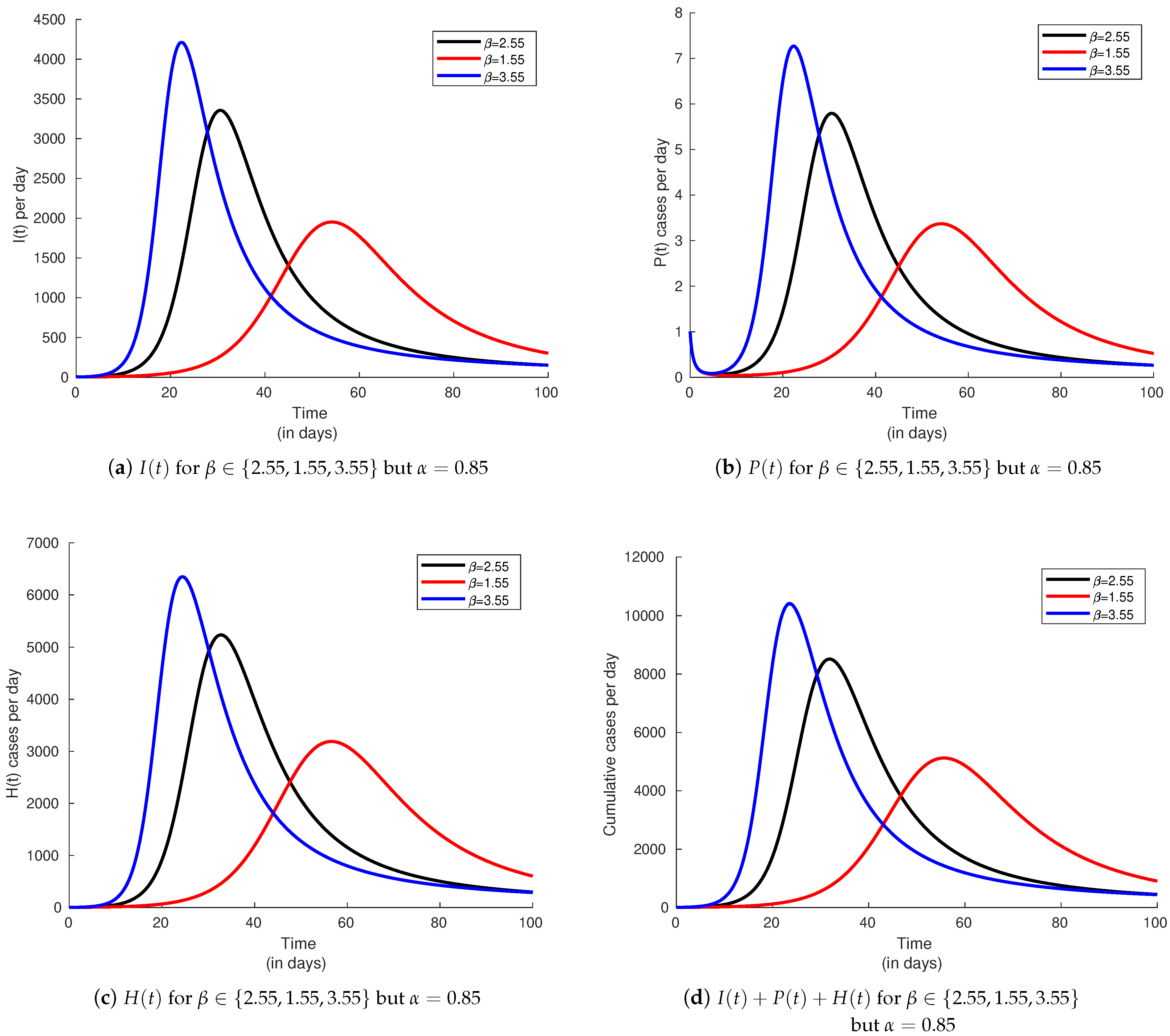
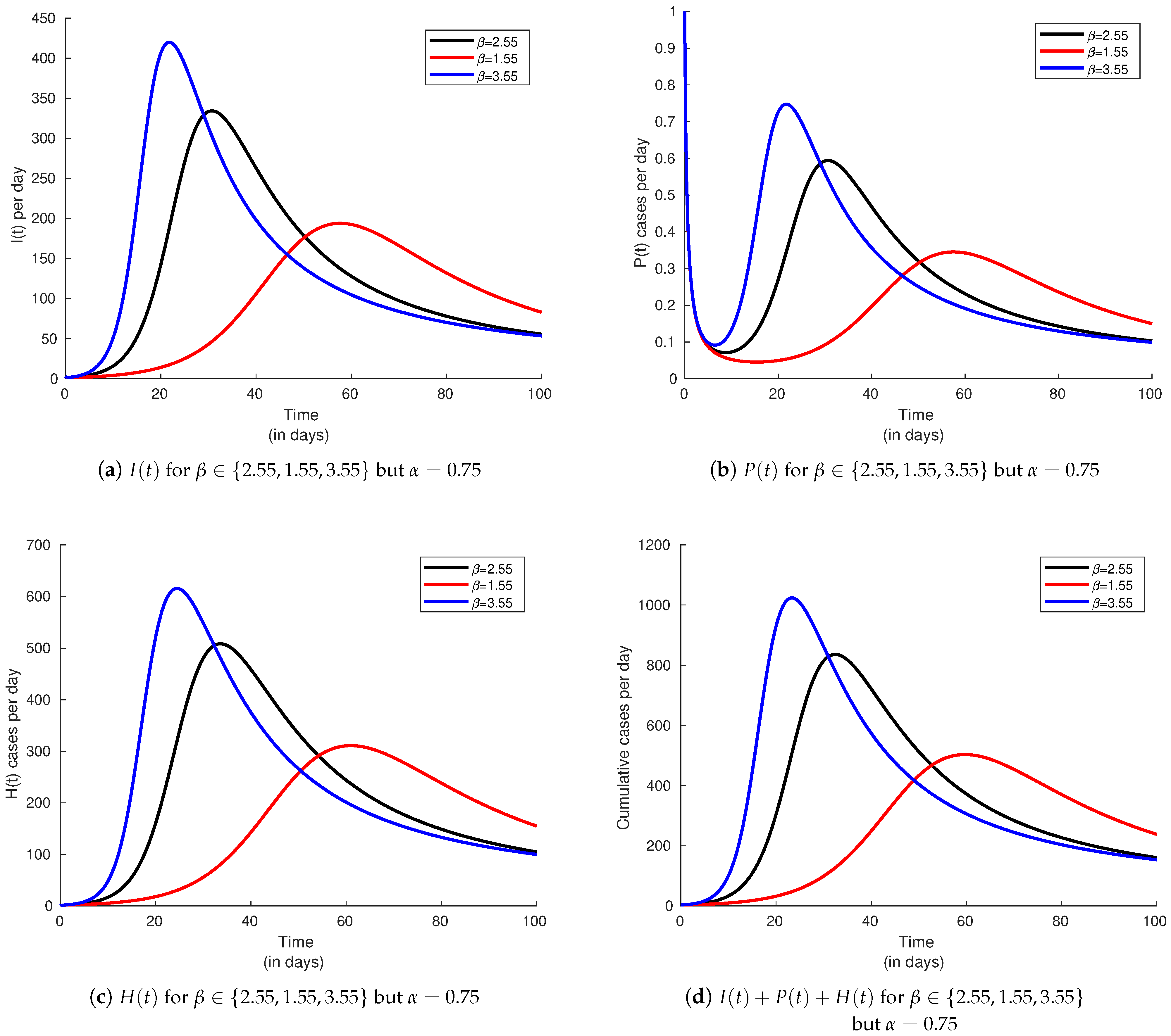
To highlight the effect of the reproduction number R 0 , from Figure 2, Figure 3 and Figure 4, three different scenarios for the infectivity rate β are considered with respect to each value of the index memory. Our results show that there is a significant decrease in the peak values of each infected categories of population when the reproduction number R 0 is reduced. For the case of super-spreaders, the curves always start with a decreasing slope and later change the peak but with lower total number of infected individuals. This makes these classes particularly special and might have a huge effect in the progression of the other infected classes. In the particular case of Portugal, it is remarkable that the peak of infected super-spreaders is less than one.

7. Conclusions

In this paper, we have analyzed in detail a fractional-order COVID-19 model, previously used for fitting the number of confirmed cases of infections from the region of Galicia, Spain, and Portugal [23]. An analytical study on the stability of the steady state was conducted and numerical simulations investigated for all infected compartments of the population. The model qualitative analysis reconfirm stability of the steady state for both classical and fractional-order models, whenever the threshold condition R 0 < 1 holds. Global stability is then deduced by a fractional-order version of LaSalle’s invariant set theorem. Moreover, our numerical solutions show that the time speed evolution for the dynamical model to reach the steady state is affected by the order α of index memory. It remains open the question of how to prove global stability in the case when R 0 > 1 . For all numerical simulations we have done, the equilibrium was always stable.

Author Contributions

Conceptualization, F.N.; methodology, F.N. and D.F.M.T.; software, F.N.; validation, F.N. and D.F.M.T.; formal analysis, F.N. and D.F.M.T.; investigation, F.N. and D.F.M.T.; writing—original draft preparation, F.N. and D.F.M.T.; writing—review and editing, F.N. and D.F.M.T.; supervision, D.F.M.T. All authors have read and agreed to the published version of the manuscript.

Funding

This research was funded by The Portuguese Foundation for Science and Technology (FCT) grant number UIDB/04106/2020 (CIDMA). Faïçal Ndaïrou was also supported by FCT through the PhD fellowship PD/BD/150273/2019.

Institutional Review Board Statement

Not applicable.

Informed Consent Statement

Not applicable.

Data Availability Statement

Not applicable.

Acknowledgments

The authors are grateful to two reviewers for their comments and suggestions.

Conflicts of Interest

The authors declare no conflict of interest. The funders had no role in the design of the study; in the collection, analyses, or interpretation of data; in the writing of the manuscript, or in the decision to publish the results.

References

  1. Oukouomi Noutchie, S.C.; Atangana, A.; Goufo, E.F.D. On the Mathematical Analysis of Ebola Hemorrhagic Fever: Deathly Infection Disease in West African Countries. BioMed Res. Int. 2014, 2014, 261383. [Google Scholar]
  2. Yanover, C.; Ngwa, G.A.; Teboh-Ewungkem, M.I. A Mathematical Model with Quarantine States for the Dynamics of Ebola Virus Disease in Human Populations. Comput. Math. Methods Med. 2016, 2016, 9352725. [Google Scholar]
  3. Yuan, S.; Rachah, A.; Torres, D.F.M. Mathematical Modelling, Simulation, and Optimal Control of the 2014 Ebola Outbreak in West Africa. Discret. Dyn. Nat. Soc. 2015, 2015, 842792. [Google Scholar]
  4. Djordjevic, J.; Silva, C.J.; Torres, D.F.M. A stochastic SICA epidemic model for HIV transmission. Appl. Math. Lett. 2018, 84, 168–175. [Google Scholar] [CrossRef] [Green Version]
  5. Duwal, S.; Winkelmann, S.; Schütte, C.; von Kleist, M. Optimal treatment strategies in the context of ’Treatment for Prevention’ against HIV-1 in resource-poor settings. PLoS Comput. Biol. 2015, 11, e1004200. [Google Scholar] [CrossRef] [Green Version]
  6. Silva, C.J.; Torres, D.F.M. A TB-HIV/AIDS coinfection model and optimal control treatment. Discret. Contin. Dyn. Syst. A 2015, 35, 4639–4663. [Google Scholar] [CrossRef]
  7. Hu, Z.; Ma, W.; Ruan, S. Analysis of SIR epidemic models with nonlinear incidence rate and treatment. Math. Biosci. 2012, 238, 12–20. [Google Scholar] [CrossRef] [PubMed]
  8. Hethcote, H.W.; van den Driessche, P. Some epidemiological models with nonlinear incidence. J. Math. Biol. 1991, 29, 271–287. [Google Scholar] [CrossRef] [PubMed] [Green Version]
  9. Moreno, V.M.; Espinoza, B.; Bichara, D.; Holechek, S.A.; Castillo-Chavez, C. Role of short-term dispersal on the dynamics of Zika virus in an extreme idealized environment. Infect. Dis. Model. 2017, 2, 21–34. [Google Scholar] [CrossRef] [PubMed]
  10. Ndaïrou, F.; Area, I.; Nieto, J.J.; Silva, C.J.; Torres, D.F.M. Mathematical modeling of Zika disease in pregnant women and newborns with microcephaly in Brazil. Math. Methods Appl. Sci. 2018, 41, 8929–8941. [Google Scholar] [CrossRef] [Green Version]
  11. Ndaïrou, F.; Area, I.; Torres, D.F.M. Mathematical Modeling of Japanese Encephalitis under Aquatic Environmental Effects. Mathematics 2020, 8, 1880. [Google Scholar] [CrossRef]
  12. Rodrigues, H.S.; Monteiro, M.T.T.; Torres, D.F.M. Seasonality effects on dengue: Basic reproduction number, sensitivity analysis and optimal control. Math. Methods Appl. Sci. 2016, 39, 4671–4679. [Google Scholar] [CrossRef] [Green Version]
  13. Kermack, W.O.; McKendrick, A.G. Contributions to the mathematical theory of epidemics I. Proc. R. Soc. Lond. 1927, 115, 700–721. [Google Scholar]
  14. Kermack, W.O.; McKendrick, A.G. Contributions to the mathematical theory of epidemics II. Proc. R. Soc. Lond. 1932, 138, 55–83. [Google Scholar]
  15. Kermack, W.O.; McKendrick, A.G. Contributions to the mathematical theory of epidemics III. Proc. R. Soc. Lond. 1933, 141, 94–112. [Google Scholar]
  16. Area, I.; Losada, J.; Ndaïrou, F.; Nieto, J.J.; Tcheutia, D.D. Mathematical modeling of 2014 Ebola outbreak. Math. Methods Appl. Sci. 2017, 40, 6114–6122. [Google Scholar] [CrossRef]
  17. Jordan, Y.A.; Smith, P. Nonlinear Ordinary Differential Equations. An Introduction to Dynamical Systems; Oxford University Press Inc.: New York, NY, USA, 1999. [Google Scholar]
  18. Melnik, A.V.; Korobeinikov, A. Lyapunov functions and global stability for SIR and SEIR models with age-dependent susceptibility. Math. Biosci. Eng. 2013, 10, 369–378. [Google Scholar]
  19. Strogatz, S.H. Nonlinear Dynamics and Chaos: With Applications to Physics, Biology, Chemistry, and Engineering; Addison-Wesley Pub: Reading, MA, USA, 1994. [Google Scholar]
  20. Teschl, G. Ordinary Differential Equations and Dynamical Systems; American Mathematical Society: Providence, RI, USA, 2012. [Google Scholar]
  21. Al-Sulami, H.; El-Shahed, M.; Nieto, J.J. On fractional order dengue epidemic model. Math. Probl. Eng. 2014. [Google Scholar] [CrossRef]
  22. Rosa, S.; Torres, D.F.M. Optimal control and sensitivity analysis of a fractional order TB model. Stat. Optim. Inf. Comput. 2019, 7, 617–625. [Google Scholar] [CrossRef] [Green Version]
  23. Ndaïrou, F.; Area, I.; Nieto, J.J.; Silva, C.J.; Torres, D.F.M. Fractional model of COVID-19 applied to Galicia, Spain and Portugal. Chaos Solitons Fractals 2021, 144, 110652. [Google Scholar] [CrossRef]
  24. Du, M.; Wang, Z.; Hu, H. Measuring memory with the order of fractional derivative. Sci. Rep. 2013, 3, 3431. [Google Scholar] [CrossRef] [PubMed]
  25. Noeiaghdam, S.; Micula, S.; Nieto, J.J. A Novel Technique to Control the Accuracy of a Nonlinear Fractional Order Model of COVID-19: Application of the CESTAC Method and the CADNA Library. Mathematics 2021, 9, 1321. [Google Scholar] [CrossRef]
  26. Rosa, S.; Torres, D.F.M. Optimal control of a fractional order epidemic model with application to human respiratory syncytial virus infection. Chaos Solitons Fractals 2018, 117, 142–149. [Google Scholar] [CrossRef] [Green Version]
  27. Boukhouima, A.; Lotfi, E.M.; Mahrouf, M.; Rosa, S.; Torres, D.F.M.; Yousfi, N. Stability analysis and optimal control of a fractional HIV-AIDS epidemic model with memory and general incidence rate. Eur. Phys. J. Plus 2021, 136. [Google Scholar] [CrossRef]
  28. Samko, S.G.; Kilbas, A.A.; Marichev, O.I. Fractional Integrals and Derivatives; Gordon and Breach Science Publishers: Yverdon, Switzerland, 1993. [Google Scholar]
  29. Kilbas, A.A.; Srivastava, H.M.; Trujillo, J.J. Theory and Applications of Fractional Differential Equations; North-Holland Mathematics Studies; Elsevier Science B.V.: Amsterdam, The Netherlands, 2006. [Google Scholar]
  30. Podlubny, I. Fractional Differential Equations; Academic Press, Inc.: San Diego, CA, USA, 1999. [Google Scholar]
  31. Sidi Ammi, M.R.; Tahiri, M.; Torres, D.F.M. Global Stability of a Caputo Fractional SIRS Model with General Incidence Rate. Math. Comput. Sci. 2021, 15, 91–105. [Google Scholar] [CrossRef] [Green Version]
  32. Lin, W. Global existence theory and chaos control of fractional differential equations. J. Math. Anal. Appl. 2007, 332, 709–726. [Google Scholar] [CrossRef] [Green Version]
  33. Almeida, R.; Brito da Cruz, A.M.C.; Martins, N.; Monteiro, M.T.T. An epidemiological MSEIR model described by the Caputo fractional derivative. Int. J. Dyn. Control 2019, 7, 776–784. [Google Scholar] [CrossRef] [Green Version]
  34. Ndaïrou, F.; Area, I.; Nieto, J.J.; Torres, D.F.M. Mathematical modeling of COVID-19 transmission dynamics with a case study of Wuhan. Chaos Solitons Fractals 2020, 135, 109846, reprinted in Chaos Solitons Fractals 2020, 141, 110311. [Google Scholar] [CrossRef]
  35. Van den Driessche, P.; Watmough, J. Reproduction numbers and sub-threshold endemic equilibria for compartmental models of disease transmission. Math. Biosci. 2002, 180, 29–48. [Google Scholar] [CrossRef]
  36. Diekmann, O.; Heesterbeek, J.A.P.; Metz, J.A.J. On the definition and the computation of the basic reproduction ratio R0 in models for infectious diseases in heterogeneous populations. J. Math. Biol. 1990, 28, 365–382. [Google Scholar] [PubMed] [Green Version]
  37. Huo, J.; Zhao, H.; Zhu, L. The effect of vaccines on backward bifurcation in a fractional order HIV model. Nonlinear Anal. Real World Appl. 2015, 26, 289–305. [Google Scholar] [CrossRef]
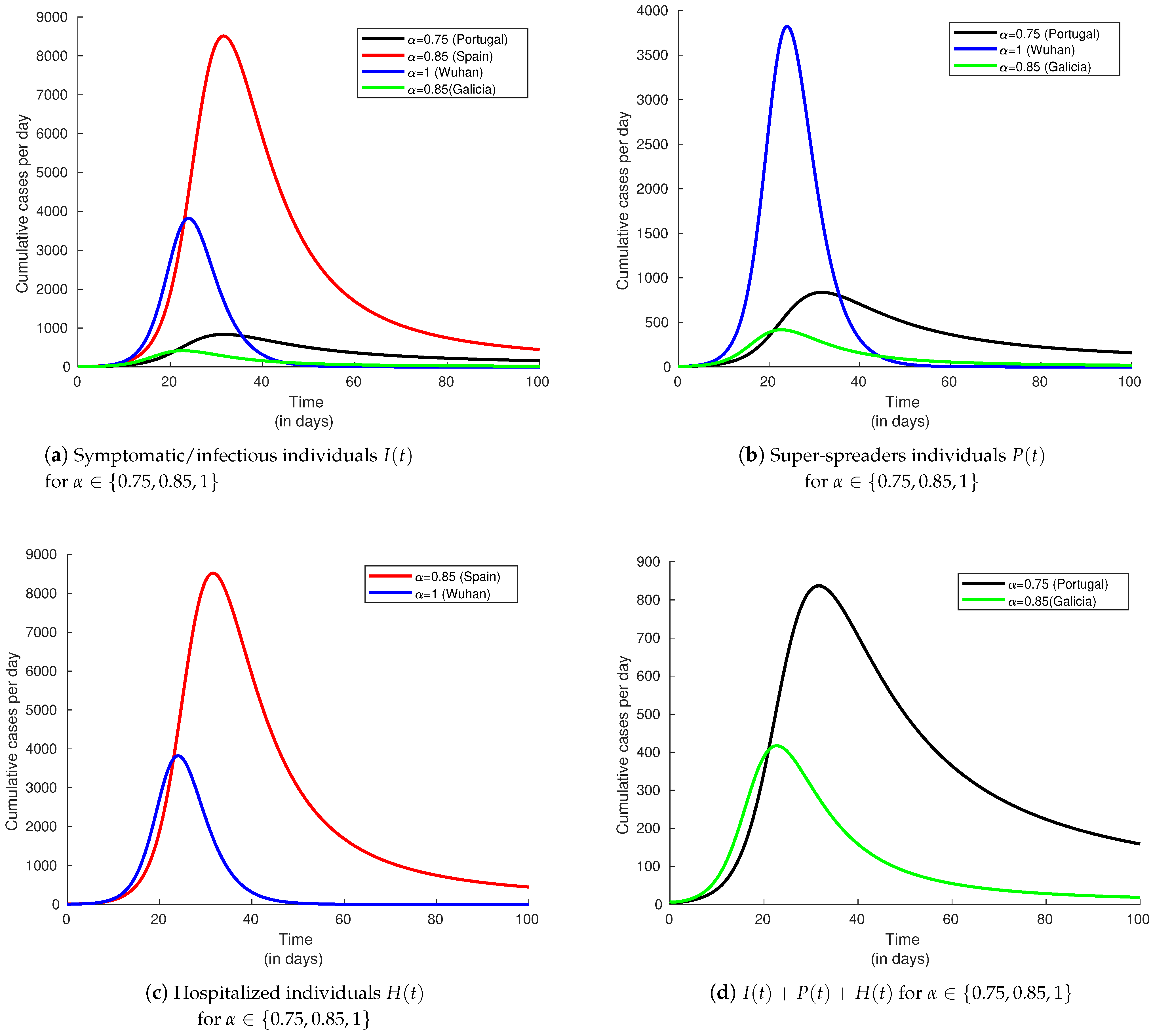
Figure 1. Evolution of infected populations by varying the order of differentiation α : the data of Portugal is well described with α = 0.75 ; the data of Spain, and Galicia alone, with α = 0.85 ; the data of Wuhan with α = 1 .
Axioms 10 00135 g001
Figure 2. Evolution of infected populations ( I ( t ) , P ( t ) , H ( t ) , and I ( t ) + P ( t ) + H ( t ) ) by varying the infectivity rate β by 1.55 , 2.55 , and 3.55 , corresponding, respectively, to the basic reproduction number 2.662 , 4.375 , and 6.088 , while fixing index memory α = 1 (Wuhan).
Axioms 10 00135 g002
Figure 3. Evolution of infected populations ( I ( t ) , P ( t ) , H ( t ) , and I ( t ) + P ( t ) + H ( t ) ) by varying the infectivity rate β by 1.55 , 2.55 , and 3.55 , corresponding, respectively, to the basic reproduction number 2.662 , 4.375 , and 6.088 , while fixing index memory α = 0.85 (Spain).
Axioms 10 00135 g003
Figure 4. Evolution of infected populations ( I ( t ) , P ( t ) , H ( t ) , and I ( t ) + P ( t ) + H ( t ) ) by varying the infectivity rate β by 1.55 , 2.55 , and 3.55 , corresponding, respectively, to the basic reproduction number 2.662 , 4.375 , and 6.088 , while fixing index memory α = 0.75 (Portugal).
Axioms 10 00135 g004
Publisher’s Note: MDPI stays neutral with regard to jurisdictional claims in published maps and institutional affiliations.