Abstract
This work proposes an interval-based uncertain Susceptible–Infected–Recovered (SIR) epidemic model. The interval model has been numerically solved by the homotopy analysis method (HAM). The SIR epidemic model is proposed and solved under different uncertain intervals by the HAM to obtain the numerical solution of the model. Furthermore, the SIR ODE model was transformed into a stochastic differential equation (SDE) model and the results of the stochastic and deterministic models were compared using numerical simulations. The results obtained were compared with the numerical solution and found to be in good agreement. Finally, various simulations were done to discuss the solution.
1. Introduction
Interval analysis is a method developed by mathematicians in the 1950s as a way of handling bounds or rounding errors and measurement errors in mathematical computation. It is useful in formulating numerical methods that yield desirable results. In short, it defines each value as a range of possibilities. This work aims to formulate interval arithmetic that solves upper and lower endpoints for the range of values of a particular function in one or more variables. These limitations are not necessarily the supremum or infimum since the exact solution of those values can be very intractable or even impossible. The treatments of interval arithmetic for real intervals of quantities with the form , where and , are permitted. The permission is based on the fact that if one of the real intervals is infinite, we would have an unbounded interval, and if both are infinite, we would have the extended real number system. Considering the classical calculation with real numbers, simple arithmetic operations and functions on elementary intervals must initially be defined. It is after this that complicated functions can be evaluated from the basic elements. In interval arithmetic, we state the range of possible outcomes explicitly.
Thus, the results are no longer stated as numbers but as intervals, which denotes imprecise values. With the size of the intervals, we express the extent of uncertainties, which are similar to error bars to a metric. The evaluations of the outer bounds of intervals are enabled by simple arithmetic operations, for example, basic arithmetic and trigonometric. Interval arithmetic was introduced by [1] as an approach to bound rounding errors in mathematical computation. The theory of interval analysis emerged considering the computation of both the exact solution and the error term as a single entity, that is, the interval. Though a simple idea, it is a very powerful technique with numerous applications in mathematics, computer science, and engineering.
In their survey, they discussed the basic concepts of interval arithmetic and some of its extensions. They also reviewed the successful application of this theory in computer science, in particular. The authors of [2] investigated the solution of linear and nonlinear ordinary differential equations with the fuzzy initial condition. They proposed two Euler-type methods to obtain a numerical solution to the problem. They also compared their solution with existing results. They observed that the results obtained were tighter than the results from the existing method. The authors of [3] also investigated the numerical solution of -th order fuzzy differential equations in the fuzzy environment using a homotopy perturbation method (HPM). They used triangular fuzzy convex normalized sets for the fuzzy parameter and variables.
They also compared their results obtained with the existing solution in terms of plots to show the efficiency of their method. The authors of [4] gave an overview of applications of interval arithmetic and discussed the verification methods for linear and nonlinear systems of equations. They also then discussed item software in the field and gave some historical remarks. The authors of [5] provided algorithms for computing the operations of interval arithmetic. They generated data that are sufficiently detailed to convert directly to a program to efficiently implement the interval operations. Finally, they extended these results to the case of general intervals, which are defined as connected sets of rules that are not necessarily closed. For this present work, we considered an interval-based uncertain epidemic model.
A related mathematical model was proposed first for SIR transmission dynamics and then the HAM was applied to find the solution. This method employs the concept of the homotopy from topology to generate a convergent series solution of nonlinear systems. The convergent series solution of nonlinear systems was enabled by utilizing a homotopy–MacLaurin series to deal with the nonlinearity in the system. The HAM is much better than most of the existing analytic approximation method because most of the existing methods are valid only for weakly nonlinear problems [6]. It overcomes the restrictions of all other analytic approximation methods and is valid for highly nonlinear problems [6]. The HAM is always valid even if small physical parameters exist or not, it provides an easy way to guarantee the convergence of approximation series, and lastly, it provides sufficient freedom to choose the equation type of sub-problems and the base function of solutions [6]. The strength of the HAM to naturally exhibit convergence of the series solution is strange in most analytic and semi-analytic approaches to nonlinear PDEs [7]. Recently, [8] used the HAM approach to solve the SIS and SIR models of [9]. The authors of [10], extended the work of [8] to solve the SIR epidemic model in the presence of a constant vaccination strategy. The authors of [7] also applied the HAM to solve the SIR epidemic model. They obtained an explicit analytic solution of the coupled nonlinear differential equations describing the epidemic model proposed. They also compared the numerical results, which showed that the two results are in good agreement. The authors of [11] studied a new approach for solving the SIR epidemic model using the HAM that was based on dividing the entire domain into subintervals.
Other works on the homotopy analysis method with the SIR model can be found in [12,13,14,15,16,17,18,19,20]. The aim of this work was to obtain the numerical solution of an interval-based uncertain SIR epidemic model using the HAM and comparing their stochastic version. The homotopy analysis method (HAM) has been applied here to study the solution of the epidemic model under uncertain intervals. The results obtained by the HAM were compared with the approximate solution and were found to be in strong agreement. We have also developed the stochastic version of the SIR epidemic model presented in this paper in order to measure the effect of randomness of the variables in the model. To the best of our knowledge, no work has been done in the area of an interval-based uncertain SIR epidemic model and very few works have been done on the stochastic model of SIR epidemic models so far. The paper is organized as follows: in Section 2, preliminaries and basic definitions are presented. In Section 3, the presentation of the proposed model is made. In Section 4, we describe the interval-based uncertain model. In Section 5, we present the homotopy analysis approach to a non-linear system, while in Section 6, we present the solution of the SIR epidemic model by the HAM. In Section 7, we present the solution, numerical results, and a discussion on the interval-based uncertain SIR epidemic model. Section 8 showcases the stochastic version of the model. In Section 9, the graphical illustrations of our results are discussed. In Section 10, the numerical solution of the SDE model are discussed. In Section 11, we present the discussion, conclusion, and possible extensions, and finally, the references are presented.
2. Preliminaries
In this section, we present some notations, definitions, and preliminaries that are used further in this paper.
- Interval Arithmetic [1]
Interval arithmetic is defined on the sets of intervals, instead of sets of real numbers. Interval arithmetic defines a set of operations on intervals, as follows:
where u and v are intervals.
- B.
- Closed Interval [1]
A closed interval, denoted by [m, n], is the set of real numbers given by
- C.
- Endpoint notation, interval equality [1]
Two intervals, A and B, are said to be equal if they are the same sets. Hence, operationally this occurs if their corresponding endpoints are equal; if and . Here , represents the left endpoint of an interval A while represents the right endpoint of an interval A, such that .
- D.
- Midpoint of A [1]
The midpoint of A is given by
- E.
- Interval Arithmetic and Operations [1]
The key point in the definition of arithmetic operations is that computing intervals are computing with sets. Let
Then, the following properties hold:
- (i)
- The sum of two intervals, A and B, is the set
- (ii)
- The difference of two intervals, A and B, is the set
- (iii)
- The product of A and B is given by
- (iv)
- The quotient of A/B is defined as
3. Model Formulation
A population comprising three kinds of individuals, denoted by S (susceptible human), I (infected human), and R (recovered human), are considered. The susceptible human ((S(t)) is the number of susceptible humans at time t, that is, humans who are vulnerable and are yet to contract the disease but have a probability of contracting it. The infected human ((I(t)) is the population of the infected and infectious persons who have the disease and can transmit it to others, while the recovered human ((R(t)) is the population of recovered humans who cannot get the disease or transmit it, because they have natural immunity, they have recovered from the disease and are immune to re-infection, they have been placed in isolation, or they have died.
The population of susceptible humans is generated through the reduction of the rate of transmission β with the infected, such that the rate of change of the population of susceptible humans is given by the following:
The rate of change of the population of infected humans is increased by the rate of transmission β with the susceptible, and reduced by the rate at which the infected population becomes isolate or recovered γ. Hence it is given by
The population of recovered humans is generated by the rate at which the infected population becomes isolated or recovered. Hence it is given by
Hence, the governing equation by [9] related to the present model is given by
Subject to the initial conditions,
4. Interval-Based Uncertain Model
As mentioned in the introduction, if we assumed that the parameters involved in a model are given in terms of an interval then it will become an interval-based model and the solution has to be handled carefully. As such, let us suppose that we have the rate of transmission β and the rate at which the infected population become isolated or recovered γ in terms of intervals and then the corresponding interval model may be written as
with the initial conditions
where S, I, and R are all now in interval form.
It may be noted from the open literature that the involved parameters, such as β and γ, are usually given in term of some ranges, so we have investigated the problem considering those ranges in terms of intervals. Hence, the intervals of β and γ are taken as the following:
- (i)
- (ii)
- .
Next, the above interval model has been solved by the homotopy analysis method (HAM). We provide, in the next section, some mathematical results.
5. Mathematical Results
We assume here that all parameters in Equation (5) are positive intervals. For the SIR model (5) to be meaningful biologically, we need to prove that all its stated variables are non-negative (except S) for all time, that is, the solutions of the Equation (5) with non-negative initial data will remain non-negative for all time .
Proposition 1.
If the initial values , then the solutions of the model (5) are non-negative for all .
Proof.
Let , We say that, from the equations of Equation (5) that
where and Therefore,
Hence,, so .
Then,
Such that
Similarly,
Hence, the solutions of the Equation (5) are non-negative (except S) for all □
Proposition 2.
Suppose Equation (5) has a unique interval-based positive solution defined on a horizon of infinite time.
Proof.
We established that Equation (5) can be rewritten in the following form:
where , so .
The functions and are . Thus, according to the Cauchy–Lipschitz theorem [21], Equation (5) has a unique positive solution on the infinite time horizon, whenever □
Corollary 1.
The compact domain is positively invariant and attracts all trajectories from Ω.
Proposition 3.
The domain Ω is positively invariant through the positive semi-wave produced by Equation (5).
Proof.
Equation (5) can be rewritten as follows:
Applying the assumption that
Thus, the field remains on the domain Ω.
In contrast, we show that by setting and as continuous intervals, such that and , if , then by the intermediate value theorem, there exists , such that . By applying the second equation of Equation (5), we obtain for , where g is the base of − Therefore, for which is a contradiction. We apply the same arguments to We show this according to Proposition 4. □
Proposition 4
([22]). Suppose is a solution of Equation (5), then , and for all .
If we add the first two equations of Equation (5) together, we obtain
Now, by applying Proposition 4 and , we have . From Proposition 4, we also have . Hence, we conclude that . From Proposition 4, we have , which implies that . Therefore, because
then
Therefore,
The quantity is positive if . From Equation (5), it is clear that and .
Hence, there exists a point , uniquely, such that and for . The point is called the equilibrium point of the first two Equations of (5) since both and vanish at . We show this according to Proposition 5.
Proposition 5
([22]). If (, is a solution of the interval base uncertain model Equation (5) then and for all .
By dividing by , which yields
therefore, . By the initial condition, we obtain
So that and
From Proposition 5, and we have that . Because , we conclude that for all We show this according to Lemma 1.
Lemma 1
([22]). Suppose be a solution of Equation (5) in the domain then and for all .
Recall that from the first equation of Equation (5) and Proposition 5, we have and we say S(t) is a decreasing function, then , such that is a finite number. Recall also from Equation (5), the third equation and we say R(t) is an increasing function. Hence, by Proposition 5,, then is a finite number. We show this according to Lemma 2.
Lemma 2
([22]). If is a solution of Equation (5), then as as , such that and are finite numbers.
Recall from Proposition 5 and from Lemma 2, So that Therefore, implies that . Then, converges. Therefore, is convergent and .
Alternately, we integrate the first equation of Equation (5):
Because and then
which implies that I(t) is integrable in the interval , and hence, . We show this according to Lemma 3.
Lemma 3
([20]). If is a solution of Equation (5) then as .
We hereby present below the procedure for the HAM for the benefit of finding the numerical solution of our interval-based uncertain model. Consider a nonlinear equation of the form
where A is a linear operator, t denotes the time, and v(t) is an unknown function. Let v0(t) denote an initial approximation of v(t) and Z denote an auxiliary linear operator [21]. We construct the zero-order deformation equation
where is the embedding parameter and is a non-zero auxiliary function. When q = 0 and q = 1, the zero-order deformation equation becomes, respectively,
and
Thus, as q increases from 0 to 1, the solution varies continuously from the initial approximation of the exact solution . Such a kind of continuous variation is called deformation in topology. Expanding by the Taylor series in the power series of q, we have
where
is the deformation derivative. If the auxiliary linear operator A, the initial approximation v0(t), the auxiliary parameter and the auxiliary function H(t) are properly chosen so that
- (i)
- the solution of the zero-order deformation Equation (6) exists for all ,
- (ii)
- the deformation derivative (11) exists for all ,
- (iii)
- the series (10) converge at q = 1,
then, we have the series solution:
Define the vector as
According to the definition (10), the governing equation can be derived from the zero-order deformation Equation (6). Differentiating (6) m-times with respect to the embedding parameter q, then by setting q = 0, and finally, dividing by m, we have the m-th order deformation equation
where
Note that according to definition (16), the right-hand side of (15) depends only on . Thus, we easily gain the series by solving the linear higher-order deformation Equation (15) using the well-known symbolic computation software such as Maple, Matlab, or Mathematica. Prediction and controlling the infection was studied in detail not only in [22] but also in other papers, for example [4,23,24,25,26,27,28,29,30,31,32,33,34,35,36]. We discuss in the next section the homotopy analysis method.
6. Homotopy Analysis Method
For this section, we solved the interval-based uncertain model (5) by considering intervals of the transmission as and the interval of recovery as , respectively. To solve the interval-based uncertain model Equation (5) by the HAM, we consider the first equation in the interval-based uncertain model Equation (5) and choose the linear operator
with the property that
where α1 is a constant of integration. The inverse operator A−1 is given by
Let the nonlinear operator be defined as
The proper selection of the auxiliary parameter and function during the implementation of the HAM method can yield uniformly valid and accurate solutions [19].
By constructing the zero-order deformation equation we have the following:
where
- (i)
- if q = 0 then ,
- (ii)
- if q = 1 then .
Therefore, we have the m-th order deformation equation
where
The solution of the m-th order deformation Equation (22) for m > 1 and using h1 = −1 and H(t) = 1 is given by
Following earlier steps, we obtain
and
where m ≥ 1 in both last equations.
7. Numerical Results and Discussion
In this section, we present the results of the homotopy analysis method for solving an interval-based uncertain model. The solutions of the interval-based uncertain model with interval and constant value γ = 0.01 in Table A1, and with interval and constant value β = 0.01 in Table A2. Table A3 and Table A4 present the minimum, maximum, and midpoints of the susceptible, infected, and recovered human population with intervals of β and γ. The results of the HAM show strong agreement with the approximation technique. In Table A3, we present the result obtained by the Runge–Kutta of fourth order method for the susceptible, infected, and recovered humans. Then, we observed that the results are in good agreement with the homotopy analysis method (HAM) in Table A4.
In Table A1, we present the result of the susceptible, infected, and recovered humans, where β is considered an interval and γ is given as a constant. In Table A2, β is considered a constant and γ is given as an interval. It is observed from Table A1 that as time increases, the lower bound (minimum) and the upper bound (maximum) are decreasing for the susceptible human population. It is also detected that the lower bound (minimum) and the upper bound (maximum) of both the infected and recovered human populations increase with time.
In Table A2, it is observed that the same situation seems to be occurring in both the lower bound (minimum) and the upper bound (maximum) for the susceptible humans. It is also noticed that the lower bound (minimum) and the upper bound (maximum) of both the infected and recovered human populations increase with time.
It is seen from Table A3 and Table A4 that the lower bound (minimum) and the upper bound of the susceptible population is decreasing with time, as seen from Table A1 and Table A2. At the same time, the lower bound (minimum) and the upper bound (maximum) of both the infected and recovered human populations increase with time. In Table A3 and Table A4, the interval denotes the center for the intervals and , while in Table A1 and Table A2, the interval represents the center for β and constant value γ. In the next section we discuss the stochastic version of the model.
8. Stochastic Version of the Model
In this part, we denote the complete probability space with a filtration with and it satisfies the condition that it is increasing and continuous while have every Q-empty sets. We introduce randomness into Equation (5) and assume that the white noise depends on the size of the corresponding populations where we applied the corresponding pattern , such that represents the intensity of the random perturbation and is a single dimensional Brownian motion that is defined on a complete probability space . Then, the stochastic model of the SIR system (5) is described by the stochastic differential equations (SDEs):
Let . Then, we can rewrite Equation (5) in the pattern of a single dimensional SDE of the form
such that , which is given by
and the function is given by
In the next section, we discuss the graphical illustration of our results.
9. Graphical Illustration of Our Results
Figure 1 shows the plot of the maximum, midpoint, and the minimum of the susceptible human intervals and . It reveals that as the maximum value is decreasing, the midpoint is also decreasing, as is the minimum point. It is clearly seen from the plot that the uncertainty lies between the upper and lower bounds. Figure 2 shows the plot of the maximum, midpoint, and the minimum of the infected human intervals and . It reveals that as the maximum value is increasing, the midpoint is also increasing, as is the minimum point. It is clearly seen from the plot that the uncertainty lies between the upper and lower bounds. Figure 3 shows the plot of the maximum, midpoint, and the minimum of the recovered human intervals and . It reveals that as the maximum value is increasing, the midpoint is also increasing, as is the minimum point. It is clearly seen from the plot that the uncertainty lies between the upper and lower bounds. We discuss in Section 10 the numerical solutions of the stochastic differential equation model.
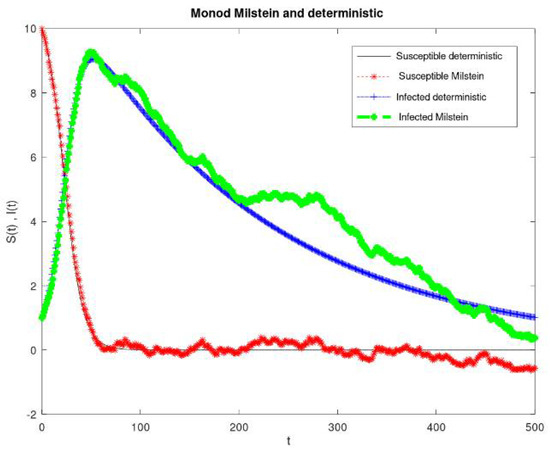
Figure 1.
Plot of the dynamic behaviors of the susceptible and infected populations under the intervals = 0.01 and = 0.01.
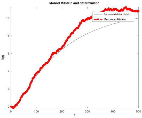
Figure 2.
Plot of the dynamic behaviors of the susceptible and infected populations under the intervals = 0.01 and = 0.01.
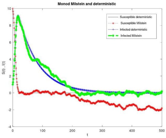
Figure 3.
Plot of the dynamic behaviors of the susceptible and infected populations under the intervals = 0.03 and = 0.015.
10. Numerical Solution of the SDE Model
In this section, we present the simulation of the SDE model (27) with the use of the Milstein method given the parameter value intervals and We obtained our numerical results of the SDE model for 500 runs of the stochastic model simulation and the results of the corresponding deterministic model are presented in Figure 1, Figure 2, Figure 3 and Figure 4, in which we display the time series solution of all the variables in the SDE model. It was obtained that in the Figure 1, Figure 2, Figure 3 and Figure 4, the SDE model simulations are lower than their deterministic model simulation.
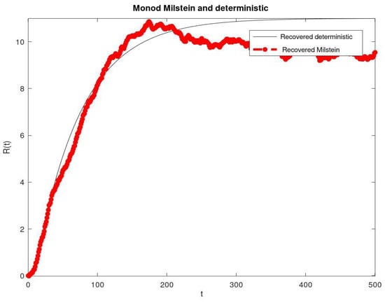
Figure 4.
Plot of the dynamic behaviors of the susceptible and infected populations under the intervals = 0.03 and = 0.015.
Figure 1 shows the simulations of the dynamic behaviors of the susceptible and the infected populations under the intervals and . It was observed that the stochastic simulations of the susceptible and the infected populations were lower than their deterministic simulations. Figure 2 shows the simulations of the dynamic behaviors of the recovered population under the intervals and . It was observed that the stochastic simulations of the recovered population were higher than their deterministic simulations. Figure 3 shows the simulations of the dynamic behaviors of the susceptible and the infected populations under the intervals and . It was observed that the stochastic simulations of the susceptible and the infected populations were lower than their deterministic simulations. Figure 4 shows the simulations of the dynamic behaviors of the recovered populations under the intervals and . It was observed that the stochastic simulations of the recovered population were lower than their deterministic simulations.
11. Discussion and Conclusions
In this work, we have studied the interval-based uncertain model of a three-compartment mathematical model rigorously. The homotopy analysis approach has been employed to solve the system of nonlinear equations of SIR interval uncertainty, in particular. The results obtained were compared with the known solution and are found to be in good agreement. Hence, it was established here that the homotopy analysis method has greater advantages over other analytical methods in many different ways. The HAM is a series expansion method that is directly dependent on small or large physical parameters, and hence, it is applicable for not only weakly but also strongly nonlinear problems. It also allows for the strong convergence of the solution over larger spatial and parameter domains. It also gives excellent flexibility in the expression of the solution and how the solution is explicitly obtained. It provides a simple way to ensure the convergence of the solution series. Comparing the stochastic and deterministic versions of the model, we saw that the population of the susceptible, infected, and recovered populations fell between the intervals obtained in the interval-based model. These suggest that the interval-based model give a very good range for the general SIR epidemic model. In the future, we plan to use fuzzy differential equations to capture the dynamics, and we also plan to look into a more practical problem that may be grounded with epidemiological data.
Author Contributions
Conceptualization, E.A.B., S.C. and R.P.; methodology, E.A.B. and S.C.; software, E.A.B.; validation, E.A.B., S.C. and R.P.; formal analysis, investigation, resources, and data curation, E.A.B.; writing—original draft preparation, E.A.B. and R.P.; writing—review and editing, S.C. and R.P.; funding acquisition, R.P. All authors have read and agreed to the published version of the manuscript.
Funding
This research received no external funding. The APC was funded by VAROPS granted by the Ministry of Defense of the Czech Republic.
Data Availability Statement
The data used to support the findings of this study are included within the article.
Acknowledgments
The authors thank the ICT Department of the Federal University Oye Ekiti, Ekiti State, Nigeria for the provision of space to complete this work and for their numerous support, as well as the Department of Science and Technology, Government of India and the Ministry of Defense of the Czech Republic for the support via the VAROPS grant.
Conflicts of Interest
The authors declare no conflict of interest.
Appendix A
The solutions obtained by the homotopy analysis method and the Runge–Kutta of the fourth order method for various intervals and and for various constant values of β and γ are stated in Table A1, Table A2, Table A3 and Table A4. Further, Figure A1, Figure A2 and Figure A3 are plotted with the maximum, center, and minimum of susceptible, infected and recovered humans under the intervals and .

Table A1.
The solutions obtained by the homotopy analysis method with the interval and the constant value of γ = 0.01.
Table A1.
The solutions obtained by the homotopy analysis method with the interval and the constant value of γ = 0.01.
| S | I | R | |||||||
|---|---|---|---|---|---|---|---|---|---|
| Time (t) | [min, max] | Midpoint of [min, max] | [β = 0.02, γ = 0.01] | [min, max] | Midpoint of [min, max] | [β = 0.02, γ = 0.01] | [min, max] | Midpoint of [min, max] | [β = 0.02, γ = 0.01] |
| 0.1 | [19.095, 19.700] | 19.396 | 19.397 | [15.270, 15.875] | 15.573 | 15.587 | [10.015, 10.015] | 10.015 | 10.015 |
| 0.2 | [18.183, 19.398] | 18.791 | 18.791 | [15.542, 16.757] | 16.150 | 16.178 | [10.031, 10.032] | 10.032 | 10.031 |
| 0.3 | [17.268, 19.097] | 18.183 | 18.182 | [15.813, 17.642] | 16.728 | 16.770 | [10.046, 10.049] | 10.048 | 10.048 |
| 0.4 | [16.357, 18.794] | 17.576 | 17.572 | [16.086, 18.524] | 17.305 | 17.363 | [10.062, 10.067] | 10.065 | 10.065 |
| 0.5 | [15.452, 18.492] | 16.972 | 16.962 | [16.358, 19.398] | 17.878 | 17.955 | [10.078, 10.086] | 10.082 | 10.082 |
| 0.6 | [14.560, 18.190] | 16.375 | 16.354 | [16.631, 20.260] | 18.446 | 18.545 | [10.095, 10.106] | 10.101 | 10.101 |
| 0.7 | [13.684, 17.887] | 15.786 | 15.749 | [16.903, 21.107] | 19.418 | 19.131 | [10.112, 10.127] | 10.120 | 10.119 |
| 0.8 | [12.828, 17.585] | 15.207 | 15.149 | [17.176, 21.932] | 19.554 | 19.712 | [10.129, 10.148] | 10.139 | 10.139 |
| 0.9 | [11.997, 17.283] | 14.640 | 14.555 | [17.447, 22.734] | 20.091 | 20.286 | [10.146, 10.170] | 10.158 | 10.159 |
| 1.0 | [11.193, 16.982] | 14.088 | 13.969 | [17.719, 23.508] | 20.614 | 20.852 | [10.164, 10.193] | 10.179 | 10.179 |

Table A2.
The solutions obtained by the homotopy analysis method with the interval and the constant value of β = 0.01.
Table A2.
The solutions obtained by the homotopy analysis method with the interval and the constant value of β = 0.01.
| S | I | R | |||||||
|---|---|---|---|---|---|---|---|---|---|
| Time (t) | [min, max] | Midpoint of [min, max] | [β = 0.02, γ = 0.01] | [min, max] | Midpoint of [min, max] | [β = 0.02, γ = 0.01] | [min, max] | Midpoint of [min, max] | [β = 0.02, γ = 0.01] |
| 0.1 | [19.699, 19.700] | 19.700 | 19.700 | [15.255, 15.286] | 15.270 | 15.270 | [10.015, 10.015] | 10.015 | 10.015 |
| 0.2 | [19.398, 19.399] | 19.399 | 19.398 | [15.511, 15.572] | 15.542 | 15.542 | [10.031, 10.032] | 10.032 | 10.031 |
| 0.3 | [19.095, 19.098] | 19.097 | 19.097 | [15.767, 15.860] | 15.814 | 15.813 | [10.046, 10.049] | 10.048 | 10.048 |
| 0.4 | [18.792, 18.797] | 18.795 | 18.794 | [16.023, 16.148] | 16.086 | 16.086 | [10.062, 10.067] | 10.065 | 10.065 |
| 0.5 | [18.489, 18.496] | 18.493 | 18.492 | [16.280, 16.437] | 16.359 | 16.358 | [10.078, 10.086] | 10.082 | 10.082 |
| 0.6 | [18.184, 18.195] | 18.190 | 18.190 | [16.536, 16.726] | 16.631 | 16.631 | [10.095, 10.106] | 10.101 | 10.101 |
| 0.7 | [17.880, 17.894] | 17.887 | 17.887 | [16.792, 17.015] | 16.904 | 16.903 | [10.112, 10.127] | 10.120 | 10.119 |
| 0.8 | [17.576, 17.594] | 17.585 | 17.585 | [17.047, 17.304] | 17.176 | 17.176 | [10.129, 10.148] | 10.139 | 10.139 |
| 0.9 | [17.272, 17.294] | 17.283 | 17.283 | [17.302, 17.593] | 17.448 | 17.447 | [10.146, 10.170] | 10.158 | 10.159 |
| 1.0 | [16.968, 16.995] | 16.982 | 16.982 | [17.556, 17.881] | 17.719 | 17.719 | [10.164, 10.193] | 10.179 | 10.179 |

Table A3.
The solutions obtained by the Runge–Kutta of the fourth order method with intervals and .
Table A3.
The solutions obtained by the Runge–Kutta of the fourth order method with intervals and .
| S | I | R | |||||||
|---|---|---|---|---|---|---|---|---|---|
| Time (t) | [min, max] | Midpoint of [min, max] | [β = 0.02, γ = 0.01] | [min, max] | Midpoint of [min, max] | [β = 0.02, γ = 0.01] | [min, max] | Midpoint of [min, max] | [β = 0.02, γ = 0.01] |
| 0.1 | [19.095, 19.699] | 19.397 | 19.397 | [15.278, 15.898] | 15.588 | 15.587 | [10.008, 10.023] | 10.015 | 10.015 |
| 0.2 | [18.180, 19.398] | 18.789 | 18.791 | [15.556, 16.804] | 16.179 | 16.178 | [10.015, 10.048] | 10.031 | 10.031 |
| 0.3 | [17.263, 19.095] | 18.179 | 18.182 | [15.835, 17.713] | 16.774 | 16.770 | [10.023, 10.073] | 10.048 | 10.048 |
| 0.4 | [16.347, 18.793] | 17.570 | 17.572 | [16.113, 18.619] | 17.366 | 17.363 | [10.031, 10.101] | 10.066 | 10.065 |
| 0.5 | [15.438, 18.490] | 16.964 | 16.962 | [16.392,19.519] | 17.956 | 17.956 | [10.039, 10.129] | 10.084 | 10.082 |
| 0.6 | 14.541, 18.187] | 16.364 | 16.354 | [16.670, 20.406] | 18.538 | 18.545 | [10.048, 10.159] | 10.103 | 10.101 |
| 0.7 | [13.659, 17.884] | 15.772 | 15.749 | [16.948, 21.277] | 19.113 | 19.131 | [10.056, 10.189] | 10.123 | 10.119 |
| 0.8 | [12.822, 17.581] | 15.202 | 15.149 | [17.225, 22.127] | 19.676 | 19.712 | [10.065, 10.222] | 10.143 | 10.139 |
| 0.9 | [11.962, 17.279] | 14.620 | 14.555 | [17.502, 22.953] | 20.227 | 20.286 | [10.073, 10.256] | 10.165 | 10.159 |
| 1.0 | [11.152, 16.976] | 14.064 | 13.969 | [17.778, 23.750] | 20.764 | 20.852 | [10.083, 10.291] | 10.186 | 10.179 |

Table A4.
The solutions obtained by the homotopy analysis method with intervals and .
Table A4.
The solutions obtained by the homotopy analysis method with intervals and .
| S | I | R | |||||||
|---|---|---|---|---|---|---|---|---|---|
| Time (t) | [min, max] | Midpoint of [min, max] | [β = 0.02, γ = 0.01] | [min, max] | Midpoint of [min, max] | [β = 0.02, γ = 0.01] | [min, max] | Midpoint of [min, max] | [β = 0.02, γ = 0.01] |
| 0.1 | [19.094, 19.699] | 19.397 | 19.399 | [15.255, 15.891] | 15.573 | 15.572 | [10.008, 10.023] | 10.015 | 10.015 |
| 0.2 | [18.181, 19.399] | 18.790 | 18.792 | [15.511, 16.789] | 16.149 | 16.148 | [10.015, 10.048] | 10.031 | 10.031 |
| 0.3 | [17.265, 19.098] | 18.181 | 18.184 | [15.767, 17.690] | 16.729 | 16.726 | [10.023, 10.073] | 10.048 | 10.048 |
| 0.4 | [16.350, 18.797] | 17.574 | 17.576 | [16.024, 18.589] | 17.307 | 17.304 | [10.031, 10.100] | 10.066 | 10.065 |
| 0.5 | [15.443, 18.496] | 16.969 | 16.968 | [16.279, 19.482] | 17.881 | 17.882 | [10.039, 10.129] | 10.084 | 10.082 |
| 0.6 | [14.547, 18.195] | 16.371 | 16.363 | [16.536, 20.363] | 18.500 | 18.457 | [10.048, 10.158] | 10.103 | 10.100 |
| 0.7 | [13.667, 17.894] | 15.780 | 15.761 | [16.792, 21.228] | 19.010 | 19.029 | [10.056, 10.189] | 10.123 | 10.119 |
| 0.8 | [12.807, 17.594] | 15.201 | 15.164 | [17.047, 22.073] | 19.560 | 19.597 | [10.065, 10.221] | 10.143 | 10.138 |
| 0.9 | [11.972, 17.294] | 14.633 | 14.573 | [17.302, 22.893] | 20.098 | 20.158 | [10.073, 10.255] | 10.164 | 10.164 |
| 1.0 | [11.164, 16.968] | 14.066 | 13.989 | [17.556, 23.686] | 20.621 | 20.712 | [10.082, 10.289] | 10.186 | 10.179 |
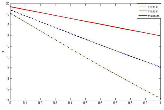
Figure A1.
Plot of the maximum, center, and minimum of susceptible humana under the intervals = [0.01, 0.03] and = [0.01, 0.015].
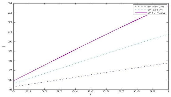
Figure A2.
Plot of the maximum, center, and minimum of infected humans under the intervals = [0.01, 0.03] and = [0.01, 0.015].
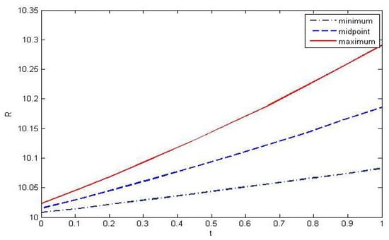
Figure A3.
Plot of the maximum, center, and minimum of recovered humans under the intervals = [0.01, 0.03] and [0.01, 0.015].
References
- Moore, R.E.R.; Baker, K.; Michael, J.C. Introduction to Interval Analysis. Society for Industrial and Applied Mathematics; Society for Industrial and Applied Mathematics: Philadelphia, PA, USA, 2009; 235p, ISBN 978-0-898716-69-6. Available online: https://1lib.cz/book/673847/09274f (accessed on 10 December 2017).
- Tapaswini, S.; Chakraverty, S. A New Approach to Fuzzy Initial Value Problem by Improved Euler Method. Fuzzy Inf. Eng. 2012, 4, 293–312. [Google Scholar] [CrossRef]
- Tapaswini, S.; Chakraverty, S. Numerical Solution of n-th Order Fuzzy Linear Differential Equations by Homotopy Perturbation Method. Int. J. Comput. Appl. 2013, 64. [Google Scholar] [CrossRef]
- Alefeld, G.; Mayer, G. Interval analysis: Theory and applications. J. Comput. Appl. Math. 2000, 121, 421–464. [Google Scholar] [CrossRef]
- Hickey, T.; Ju, Q.; van Emden, M.H. Interval Arithmetic: From Principles to Implementation. J. ACM 2001, 48, 1038–1068. [Google Scholar] [CrossRef]
- Liao, S.J. Homotopy Analysis Method. Available online: https://numericaltank.sjtu.edu.cn/IntroductionHAM.htm (accessed on 27 May 2021).
- Hayat, T.; Sajid, M. Homotopy analysis of MHD boundary layer flow of an upper-convected Maxwell fluid. Int. J. Eng. Sci. 2007, 45, 393–401. [Google Scholar] [CrossRef]
- Khan, H.; Mohapatra, R.N.; Vajravelu, K.; Liao, S. The explicit series solution of SIR and SIS epidemic models. Appl. Math. Comput. 2009, 215, 653–669. [Google Scholar] [CrossRef]
- Kermack, W.O.; McKendrick, A.G. A contribution to the mathematical theory of epidemics. Proc. R. Soc. Lond. Ser. A Math. Phys. Sci. 1927, 115, 700–721. [Google Scholar] [CrossRef]
- Momoh, A.A.; Ibrahim, M.O.; Tahir, A.; Adamu, I.I. Application of homotopy analysis method for solving the SEIR models of epidemics. Nonlinear Anal. Differ. Equ. 2015, 3, 53–68. [Google Scholar] [CrossRef]
- Motsa, S.S. The homotopy analysis method solution of SIR epidemic model. J. Adv. Res. Differ. Equ. 2010, 2, 1–9. [Google Scholar]
- Bataineh, A.S.; Noorani, M.S.M.; Hashim, I. Series Solution of the Multispecies Lotka-Volterra Equations by Means of the Homotopy Analysis Method. Differ. Equ. Nonlinear Mech. 2008, 2008, 816787. [Google Scholar] [CrossRef]
- Ghotbi, A.R. Homotopy analysis method for solving the MHD flow over a non-linear stretching sheet. Commun. Nonlinear Sci. Numer. Simul. 2009, 14, 2653–2663. [Google Scholar] [CrossRef]
- Odibat, Z.; Bataineh, A.S. An adaptation of homotopy analysis method for reliable treatment of strongly nonlinear problems: Construction of homotopy polynomials. Math. Methods Appl. Sci. 2015, 38, 991–1000. [Google Scholar] [CrossRef]
- Shivanian, E.; Abbasbandy, S. Predictor homotopy analysis method: Two points second order boundary value problems. Nonlinear Anal. Real World Appl. 2014, 15, 89–99. [Google Scholar] [CrossRef]
- Jafari, H.; Firoozjare, M.A. Multistage Homotopy Analysis Method for Solving Nonlinear Integral Equations. Appl. Appl. Math. Int. J. 2010, 34–45. Available online: https://www.pvamu.edu/aam/special-issues/august-2010/ (accessed on 10 December 2017).
- Sadaf, M.; Akram, G. An improved adaptation of homotopy analysis method. Math. Sci. 2017, 11, 55–62. [Google Scholar] [CrossRef]
- Liao, S. Homotopy analysis method—A new analytic approach for highly nonlinear problems. AIP Conf. Proc. 2015, 1648, 020011. [Google Scholar] [CrossRef]
- Liao, S.J. Beyond Perturbation: Introduction to Homotopy Analysis Method; Chapman and Hall/CRC Press: Washington, DC, USA, 2003. [Google Scholar]
- Noeiaghdam, S.; Araghi, M.A.F. Application of the CESTAC Method to Find the Optimal Iteration of the Homotopy Analysis Method for Solving Fuzzy Integral Equations. In Progress in Intelligent Decision Science; Springer: Cham, Switzerland, 2020. [Google Scholar] [CrossRef]
- Soltani, L.A.; Shivanian, E.; Ezzati, R. Convection–radiation heat transfer in solar heat exchangers filled with a porous medium: Exact and shooting homotopy analysis solution. Appl. Therm. Eng. 2016, 103, 537–542. [Google Scholar] [CrossRef]
- Rachah, A.; Torres, D.F.M. Predicting and controlling the Ebola infection. Math. Methods Appl. Sci. 2016, 40, 6155–6164. [Google Scholar] [CrossRef]
- Mengxin, H.; Zhong, L.; Fengde, C.; Zhenliang, Z. Dynamic Behaviors of an N-species Lotka-Volterra Model with Nonlinear Impulses. IAENG Int. J. Appl. Math. 2020, 50, 22–30. [Google Scholar]
- Ayub, M.; Zaman, H.; Sajid, M.; Hayat, T. Analytical solution of stagnation-point flow of a viscoelastic fluid towards a stretching surface. Commun. Nonlinear Sci. Numer. Simul. 2008, 13, 1822–1835. [Google Scholar] [CrossRef]
- Holub, M.; Bradac, F.; Pokorny, Z.; Jelinek, A. Application of a Ballbar fordiagnostics of CNC machine tools. MM Sci. J. 2018, 2601–2605. [Google Scholar] [CrossRef]
- Biazar, J. Solution of the epidemic model by Adomian decomposition method. Appl. Math. Comput. 2006, 173, 1101–1106. [Google Scholar] [CrossRef]
- Hethcote, H.W. The Mathematics of Infectious Diseases. SIAM Rev. 2000, 42, 599–653. [Google Scholar] [CrossRef]
- Bakare, E.; Hoskova-Mayerova, S. Optimal Control Analysis of Cholera Dynamics in the Presence of Asymptotic Transmission. Axioms 2021, 10, 60. [Google Scholar] [CrossRef]
- Vagaska, A.; Gombar, M. Mathematical Optimization and Application of Nonlinear Programming. In Algorithms as a Basis of Modern Applied Mathematics; Springer Nature: Cham, Switzerland, 2021; pp. 461–486. ISBN 978-3-030-61333-4. [Google Scholar] [CrossRef]
- Efimov, D.; Ushirobira, R. On an interval prediction of COVID-19 development based on a SEIR epidemic model. Annu. Rev. Control 2021. preprint. Available online: https://hal.inria.fr/hal-02517866v4 (accessed on 27 May 2021). [CrossRef] [PubMed]
- Li, C.; Huang, J.; Chen, Y.-H.; Zhao, H. A Fuzzy Susceptible-Exposed-Infected-Recovered Model Based on the Confidence Index. Int. J. Fuzzy Syst. 2021, 1–11. [Google Scholar] [CrossRef]
- Bao, K.; Rang, L.; Zhang, Q. Analysis of a stochastic SIRS model with interval parameter. Am. Inst. Math. Sci. (AIMS) 2019, 24, 4827–4849. [Google Scholar] [CrossRef]
- Park, S.W.; Champredon, D.; Weitz, J.S.; Dushoff, J. A Practical Generation Interval-Based Approach to Inferring the Strength of Epidemics from Their Speed. 2018. Available online: https://www.biorxiv.org/content/10.1101/312397v2.full.pdf (accessed on 28 May 2021).
- Bracher, J.; Ray, E.L.; Gneiting, T.; Reich, N.G. Evaluating epidemic forecasts in an interval format. PLoS Comput. Biol. 2021, 17, e1008618. [Google Scholar] [CrossRef]
- Bhuju, G.; Phaijoo, G.R.; Gurung, D.B. Fuzzy Approach Analyzing SEIR-SEI Dengue Dynamics. BioMed Res. Int. 2020, 2020, 1508613. [Google Scholar] [CrossRef]
- Dhandapani, P.B.; Baleanu, D.; Thippan, J.; Sivakumar, V. On stiff, fuzzy IRD-14 day average transmission model of COVID-19 pandemic disease. AIMS Bioeng. 2020, 7, 208–223. [Google Scholar] [CrossRef]
Publisher’s Note: MDPI stays neutral with regard to jurisdictional claims in published maps and institutional affiliations. |
© 2021 by the authors. Licensee MDPI, Basel, Switzerland. This article is an open access article distributed under the terms and conditions of the Creative Commons Attribution (CC BY) license (https://creativecommons.org/licenses/by/4.0/).