Abstract
Entrepreneurship is a theme of global interest, and it is the subject of investigations conducted by many researchers and projects. In particular, the Global Entrepreneurship Monitor project is a global project that involves several countries and years of surveys on entrepreneurship indicators. This study focuses on the 12 indicators of the entrepreneurial ecosystem defined by the Entrepreneurial Framework Conditions (EFCs). The EFCs are specifically related to the quality of the entrepreneurial ecosystem. Using clustering techniques, the present study analyzes how European experts’ perceptions on the EFCs of their home country have changed between 2000 and 2019. The main finding is the existence of significant differences between the clusters obtained over the years and between countries. Therefore, in theoretical terms, this dynamical behavior in relation to the entrepreneurial conditions of economies should be considered in future works, namely, those concerning the definition of the number of clusters, which, according to the internal validation measures computed in this work, should be two.
MSC:
62H30; 62P20; 91-10
1. Introduction
In the last decades, the topic of entrepreneurship has gained increasing attention. Political leaders viewed entrepreneurial activity as a source of innovation, competitiveness and economic development, and academics set about deepening the knowledge about this core topic, resulting in it now representing a hybrid field comprised of different perspectives and theories [1]. Entrepreneurship is explained as an individual’s ability to place ideas into practice; articulate project planning and management; take calculated risks; innovate; and creative with the purpose of achieving previously defined goals [2]. Thus, is it suggested that entrepreneurship may be a catalyst for economic growth and national competitiveness. In fact, as [3] explain in their extensive systematic literature review on entrepreneurial ecosystems, the growing interest in this topic is being guided largely by the interest demonstrated by policy makers in increasing entrepreneurial activity via the creation of new companies and promotion of self-employment.
The Global Entrepreneurship Monitor (GEM) research project, funded in 1997, is the largest ongoing study of entrepreneurial dynamics in the world [4]. The first report of this project was launched in 1999 and encompassed 10 developed economies—eight from the OECD (Canada, Denmark, Finland, France, Germany, Israel, Italy and the United Kingdom) as well as Japan and the United States of America [4], and it has grown to include a wide amount of economies over the world [5]. According to the GEM 2019/2020 Global Report, fifty economies participated in the GEM 2019 adult population survey, including 21 European countries.
The GEM survey is based on collecting primary data through an adult population survey (APS) of at least 2000 randomly selected adults (18–64 years of age) in each economy. Additionally, national teams collect experts’ opinions about components of the entrepreneurship ecosystem through a national expert survey (NES) [4].
The present study focus on the 12 indicators compiled by the NES survey data concerning the entrepreneurial ecosystem defined by GEM, i.e., the Entrepreneurial Framework Conditions (EFCs), detailed in Table A1 in Appendix A.
Although the original GEM model expects national business activity to change with general national framework conditions, studies show that entrepreneurial activity varies according to the EFCs [2]. In line with that result, the aim of the present work is to study the changes that have occurred in the European experts’ perceptions over the last two decades (between 2000 and 2019) in different countries.
There are already several studies that use GEM data in their research. Recently, [2], explained the entrepreneurial performance of economies taking into account the variables present in the EFCs combining factorial analysis with cluster analysis to group economies (countries). In addition, Pilar et al. [6] analyzed entrepreneurs’ perceptions about conditions to create new and growing firms and their significance in the economic development level (EDL) of countries, using NES 2013. Braga et al. [7] analyzed GEM data in order to understand what leads certain countries’ individuals to display higher levels of initiative to manage or create a high-growth business. In [8], NES datasets for 2011 until 2013 were analyzed to study the effects of different types of entrepreneurship expert specialization on the perceptions about the EFCs. Furthermore, the work of Autio et. al [9] also contributed to the understanding of the theoretical, managerial and policy implications of entrepreneurial innovation using GEM data.
Based on the similarities in economic performance across European countries, this study is mainly concerned with the evolution of experts’ perceptions on the entrepreneurial framework in Europe, grouping countries in different clusters and analyzing how this grouping differs throughout the years. To achieve this goal, the present study uses multivariate cluster analysis to group all European economies according to the experts’ perceptions on the EFCs of their home country (similarly to the methodology adopted by [2]). In the next section, the dataset, methods and results are presented, and in the last section, the discussion is given and future research directions are suggested.
2. Materials and Methods
2.1. Dataset
For citizens to become entrepreneurs, the conditions for entrepreneurship in their countries must be favorable. The GEM conceptual framework is based on the assumption that national economic growth is the result of the inter-dependencies between the EFCs and the personal traits and capabilities of individuals to identify and seize opportunities [10]. Thus, the behavior of these GEM indicators over the last two decades in Europe (between 2000 and 2019) are studied in this work. Although they do not directly measure the real conditions of the country, they measure them indirectly through the European experts’ perceptions.
The two main sources of primary data of the GEM project are as follows:
- The adult population survey (APS), which provides standardized data on entrepreneurial activities and attitudes within each country—at least 2000 randomly selected adults (18–64 years of age)in each economy.
- The national expert survey (NES) investigates the national framework conditions for entrepreneurship by means of standardized questionnaires; national teams collect experts’ opinions about components of the entrepreneurship ecosystem through a national expert survey.
In a previous study [11], the period from 2010 to 2016 was analyzed. Substantial changes in the clusters of European economies through these years were observed. In particular, it was found that despite the economic and financial similarities between Portugal, Italy, Greece and Spain, countries that all faced a dramatic period between 2010–2012, Portugal took off from the remaining countries after 2012, and only in 2016 was it caught up by Spain.
The present study aims at extending that work by considering the period before the crisis and after 2016 in order to obtain a wider view on European entrepreneurs’ perceptions. For such purpose, multivariate cluster analysis techniques are used to group all of the European economies according to the experts’ perceptions on the EFCs of their home country.
Therefore, the present study considers the 12 indicators of the entrepreneurial ecosystem, i.e., the EFCs, defined by the GEM project, for the whole the period of available data, namely from 2000 until 2019. The description of the EFCs is given in Table A1 in Appendix A.
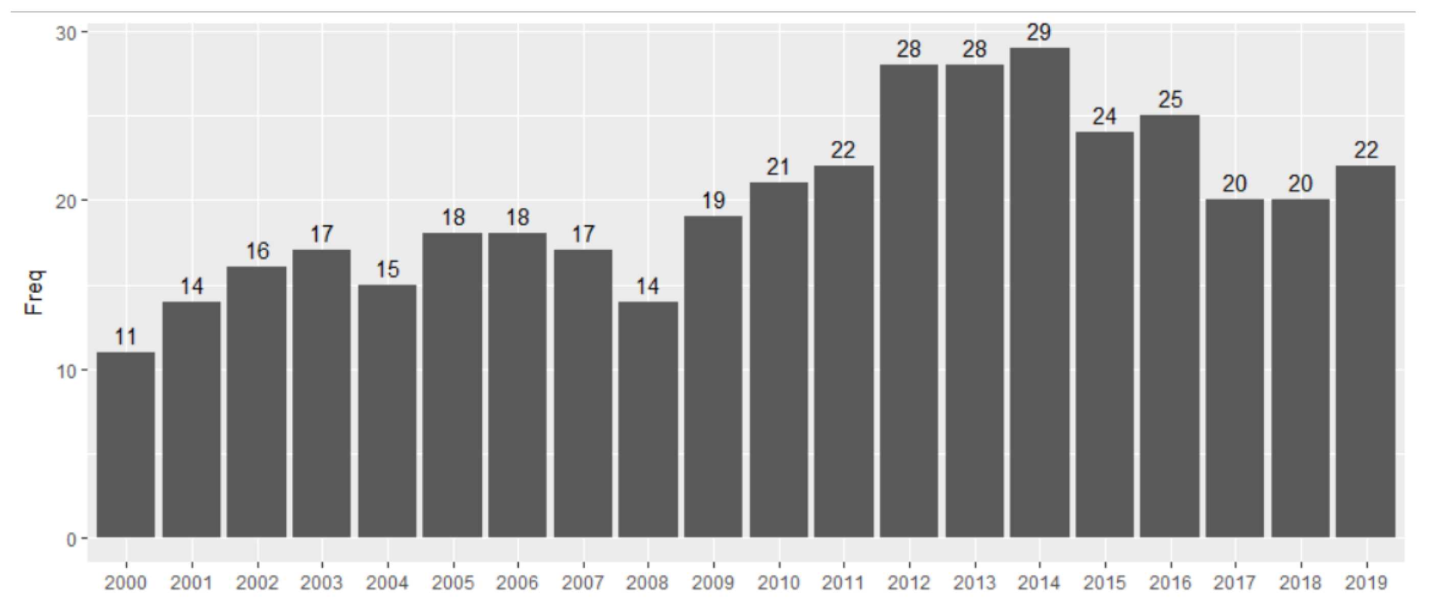
The number of economies that participated in the NES survey between 2000 and 2019 ranges from a minimum of 11 countries in 2000 to a maximum of 29 countries in 2014 (see Figure 1).
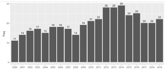
Figure 1.
Number of economies in NES survey between 2000 and 2019.
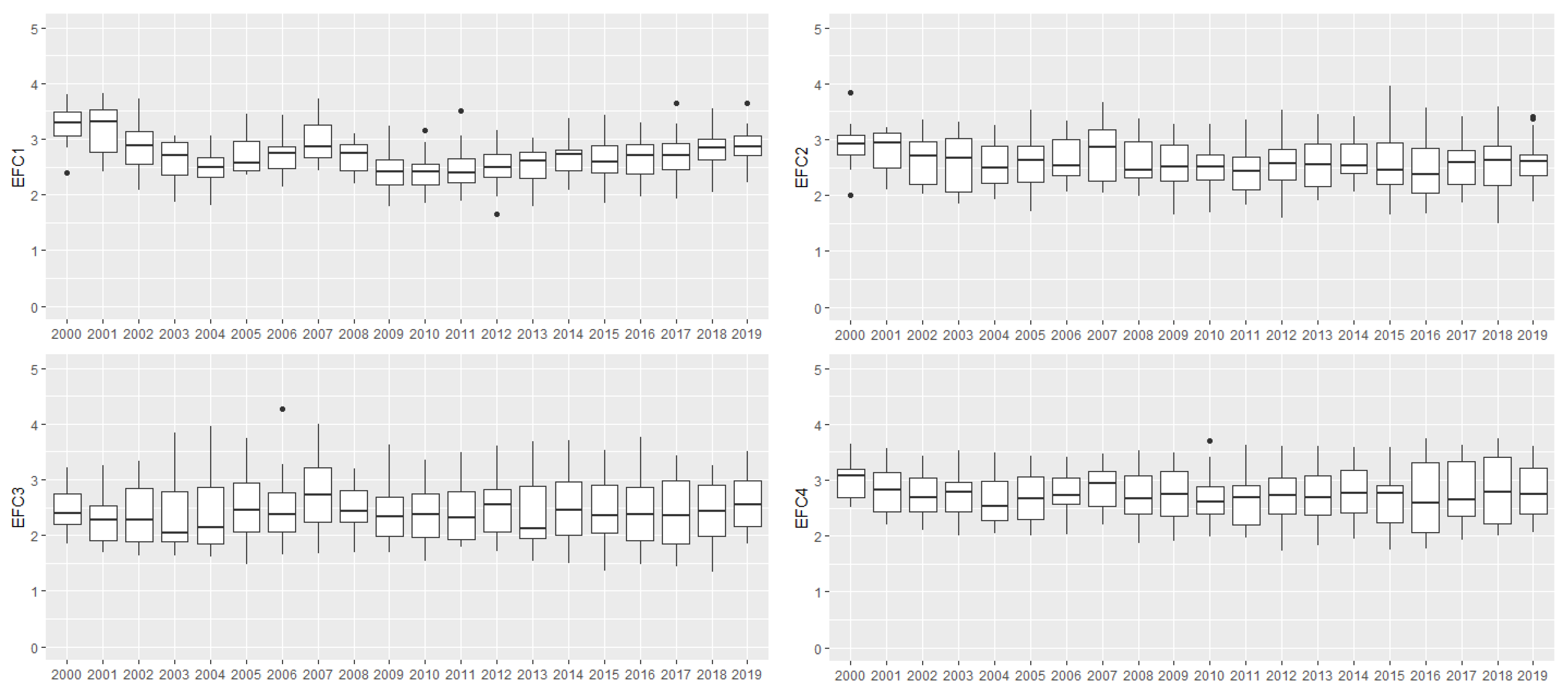
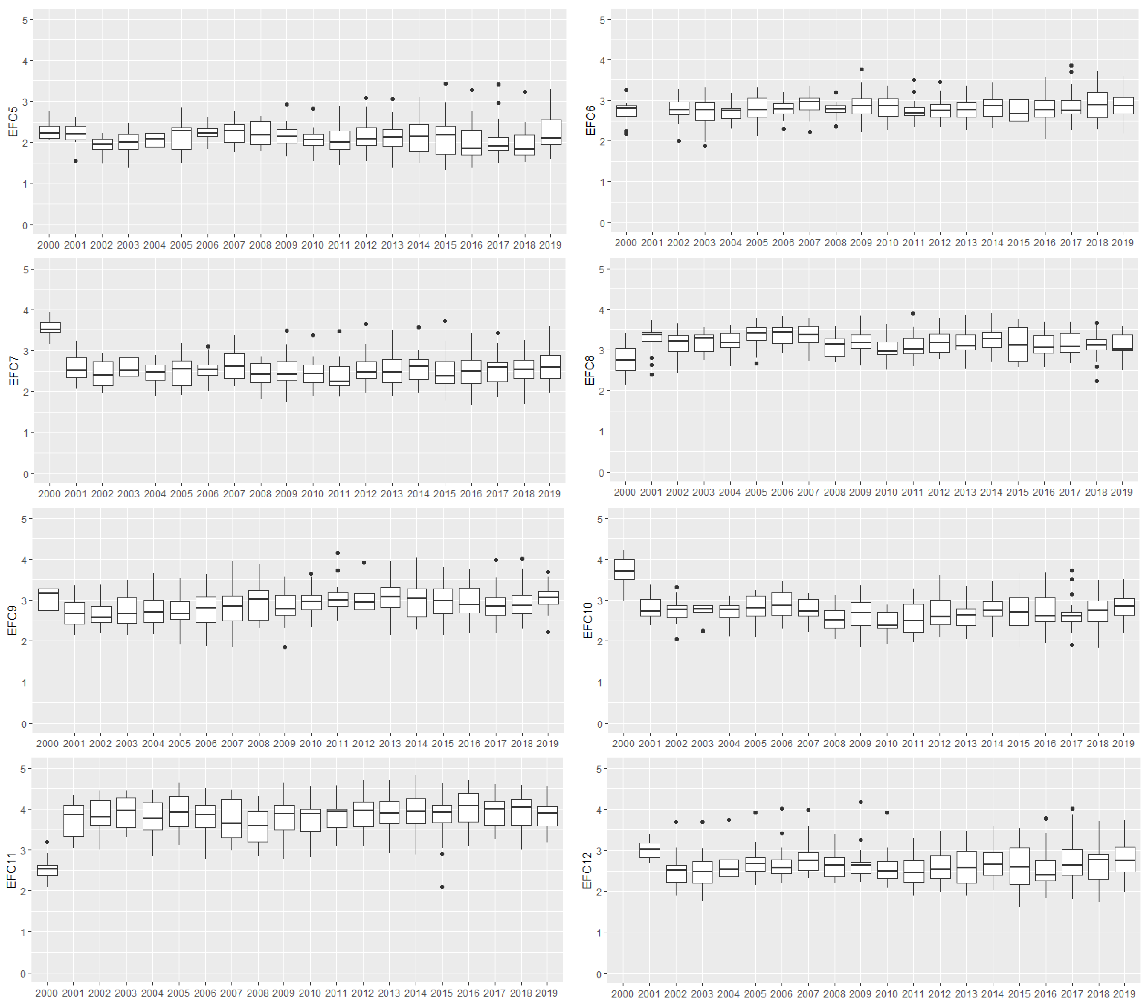
Figure 2 illustrates the variation of each EFCs throughout the years and between countries. In general, large amplitudes, as observed for EFCs 2, 3, 4 and 11, reflect the differences in intra-country perceptions. The longitudinal volatility of the median, easily observed in EFCs 1, 8, 11 and 12, illustrates the annual differences in perceptions. This means that an intra-annual and intra-country difference is to be expected. The purpose of this study is to detect these differences by analyzing how countries are grouped, according to similar perceptions, over the years in the last two decades.
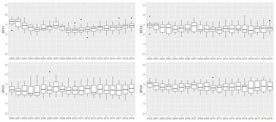
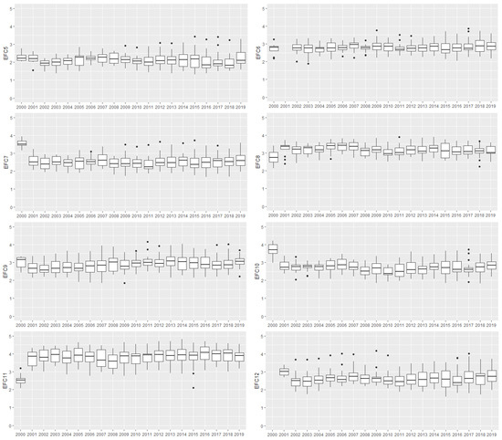
Figure 2.
Box plots of the 12 EFCs in the period of 2010–2019.
2.2. Methodology
Cluster analysis includes several multivariate statistical procedures that can be used to classify objects or individuals into relatively homogeneous groups (clusters), taking into account similarities or dissimilarities between them. Sokal and Sneath presented the most popular application of these methodologies in the book [12] as early as 1963 for biological classification of species. From then on, the use of classification techniques became common practice in the most diverse of areas: in medicine to classify diseases, in the social sciences to define homogeneous cultural and scientific areas [13,14,15] and in marketing for segmenting markets and customers [16,17], among others.
Given a set of n individuals for whom there is information on the form of p variables, a method of cluster analysis proceeds to group individuals according to the existing information in such a way that individuals belonging to the same group are as similar as possible and always more similar to the elements of the same group than to elements of the other groups [18].
An initial difficulty in cluster analysis is that there is no single criterion, similarity measure or technique for defining the groups. The literature on the subject, as well as the available statistical packages, presents us with a very wide range of criteria, always aiming to obtain coherent groups that are significantly different from each other.
The choice of clustering technique depends on the type of variables to be considered (continuous, ratios, ordinal, nominal or binary) and must take into account different scales of measurement of the variables. In this case, it is common practice to standardize the variables, because any measure of similarity/dissimilarity will reflect the weight of the variables that have higher values and dispersion; thus, it is advisable that the variables have the same unit of measure.
Cluster analysis methods can be grouped into four types [18]:
- Optimization techniques—based on the early choice of a number of clusters, k, and a division of all cases is made by the pre-established k groups. Next, the optimization of the chosen criterion is performed. In general, it is intended that within each group, the elements are as similar as possible and as different as possible from elements in other groups;
- Hierarchical techniques—based on a matrix of similarities (or differences) in which each element of the matrix describes the degree of similarity (or difference) between each two cases, based on the chosen variables. These techniques can be agglomerative or divisive. In the first case, the procedure starts with n groups including one individual that are grouped successively until only one group is obtained including all n individuals. In the divisive, 0 the reverse process is applied: one starts from a group with all of the individuals and successive divisions are applied until obtaining n groups;
- Density or mode-seeking techniques—groups are formed by looking for regions that contain a relatively dense concentration of cases.
- Other techniques—these include those that allow groups to overlap (fuzzy clusters), additive partitive methods (kmeans and hill climbing), those that do not use a similarity matrix but that can be directly applied to the original data and others that are not included in the previous types;
Furthermore, there are several measures that can be used as measures of distance or dissimilarity between the elements of a data matrix. The most used distances are as follows:
- Euclidean distance between two cases (i and j) is the square root of the sum of the squares of the differences between values of i and j for all variables (), that is,
- Minkowski distance can be considered as a generalization of Euclidean distance (coincide when r = 2):
- Mahalanobis distance considers the covariance matrix for the calculation of distanceswhere and are the vectors of variable values for individuals i and j, respectively.
Considering the matrix of observed data , where is the value of variable for individual . For a population of dimension N, the covariance matrix is given as
where row u, for individual u, of the matrix X is the vector of the p variables under study, i.e.,
and is the vector of the population means.
Other similarity indices can also be used, as long as they respect the following metric properties: symmetry, triangular inequality, differentiability of non-identicals and indifferentiability of identicals.
The indices used include, in addition to distances, correlation coefficients, association coefficients and probabilistic similarity measures, according to [19]. The correlation coefficients are more suitable if the variables have different scales and dispersion, the association coefficients are particularly useful when the variables are binary qualitative, and the probabilistic similarity measures are only used if the similarity index is to be the probability gaining information based on the initial variables.
Therefore, different definitions of distances may result in different final solutions for grouping individuals.
At each step of the agglomerative process, the similarity/distances matrix is recalculated, and the recurrence (Equation (4)) must be satisfied:
where is the distance between the group k and the group formed by the junction of the groups (or elements) i and j.
Although the recurrence equation is always the same, the coefficients and differ according to the agglomerative method or criterion. The agglomerative method or criterion can be the following:
- Single linkage or criterion of the nearest neighbor, for which the similarity between two groups is the maximum similarity between any two cases belonging to those groups. That is, for the two groups (i, j) and (k), the distance between the two is given by Equation (5).In this case, the coefficients in recurrence Equation (4) are
- Complete linkage or the criterion of the furthest neighbor uses the process inverse to the previous one; that is, given two groups, the distance between the two is given by Equation (6).In this case, the coefficients in recurrence Equation (4) are
- Average defines the distance as the average of the distances between all pairs of individuals constituted by elements of the two groups. This strategy is, in a way, intermediate in relation to the first two described.In this case, the coefficients in recurrence Equation (4) are
- Centroid defines the distance between two groups as the distance between their centroids, points defined by the means of the variables that characterize the individuals in each group.In this case, the coefficients in recurrence Equation (4) are
- Ward method [20] is based on the loss of information resulting from the grouping of individuals and measured by adding the squares of the deviations from individual observations relative to the averages of the groups in which they are classified.In this case, the coefficients in recurrence Equation (4) are
There is no better criterion for (dis)aggregation of cases in cluster analysis. It is common practice to use several criteria and to compare the results. If these are similar, it is possible to conclude that the results have been obtained with a high degree of stability and, therefore, that they are reliable [18].
Another problem with cluster analysis is the adequate number of clusters to consider. Sometimes, there is prior knowledge, on the part of the researcher, of the number of groups in which the study population should be divided; in which case, this information can be used.
Other criteria for defining the number of clusters that can be used are major changes in the fusion coefficient, the co-phenetic correlation values, the comparison of the application of different numbers of clusters and the comparison of the similarity of the results obtained, the degree of convergence of methods and internal and external validation measures.
The connectivity measure, proposed by Handl et al. in [21], the Dunn index [22] and Silhouette Width [23] are the main internal validation measures.
Given a set of n individuals for whom there is information on the form of p variables, the is defined by Equation (7):
where is the jth nearest neighbor of observation i,
is a partition of the n observations into k disjoint clusters and l is a parameter giving the number of nearest neighbors to use, [21]. This measure has values between 0 and ∞ and should be minimized.
The Dunn Index [22] is given by Equation (8),
where is the maximum distance between observations in cluster . This measure has values between 0 and ∞ and should be maximized.
Silhouette Width [23] is given by Equation (9):
where is the average distance between i and all other observations, such as
where is the cluster containing observation i, is the considered distance between observations i and j, and is the cardinality of cluster C. This measure has values between and 1 and should be maximized.
These measures are implemented by Brock et al. [24] in the package clValid. This package comprises the internal validation measures and, in addition, the stability and biological validation measures. Internal validation measures take only the dataset and the clustering partition as input and use intrinsic information in the data to assess the quality of the clustering. The stability measures are a special version of internal measures. They evaluate the consistency of a clustering result by comparing it with the clusters obtained after each column is removed, one at a time. Biological validation evaluates the ability of a clustering algorithm to produce biologically meaningful clusters.
There are several cluster validation measures defined in the literature [25,26,27,28]. It is not possible to obtain the best result always with the same validation measure. Thus, several authors have proposed merging several validation measures, such as the Davies–Bouldin index, the Calinski–Harabasz index and the Dunn index, which allow for comparisons of several solutions and the selection of the internal optimal solution [26,27,28]. However, these validation measures focus on internal validation, but it is also important to take into account the external ones. For this reason, hybrid validation measures that combine these two types of validation have been emerging and are described by Gajawada and Toshniwal (2012) [29]. Improved measures have also been proposed based on the most common ones already mentioned; for example, since the numerical procedure to calculate the Silhouette Width criterion is rather demanding, the Simplified Silhouette Width Criterion (SSWC)—which instead of the average value, uses the distance between the elements and the clusters centroids, thus deeming the partition with the largest SSWC index to be the most appropriate partition—is usually applied [28].
3. Results and Discussion
In order to study the European countries based on the EFCs experts’ perceptions during the period of 2000–2019, cluster analysis was used to group the countries into homogeneous groups. As discussed in Section 2, several measures and methods can be used for grouping countries.
In [11], the hierarchical cluster technique, Euclidean distance and the Ward method were used in order to analyze, for the period of 2010–2016, European entrepreneurs’ perceptions. The present study considers the whole period of available data (between 2000 and 2019), extending that work. In that previous work, the statistical software R version 3.4.0 was used, and three clusters were considered, justified by GEM project’s definition of economic development level, which considers three types of economies: (i) economies driven by factors of production; (ii) efficiency-oriented economies; and (iii) innovation-oriented economies. It was found that for each year, the countries that constitute each of the clusters observe substantial changes in the clusters throughout the years. In particular, while in 2010 and 2011 Portugal was in clusters with the second-best overall average EFCs perceptions, in 2012, Portugal was in the group with the lowest EFCs perceptions. However, from 2013 to 2016, Portugal recovered in terms of experts’ perceptions and moved into the group with the second-best overall average. The behavior of Portugal was compared with that of Italy, Greece and Spain.
Considering the complete set of data, the present work intends to study the behavior of the European Expert’s perceptions about their economies’ entrepreneur conditions.
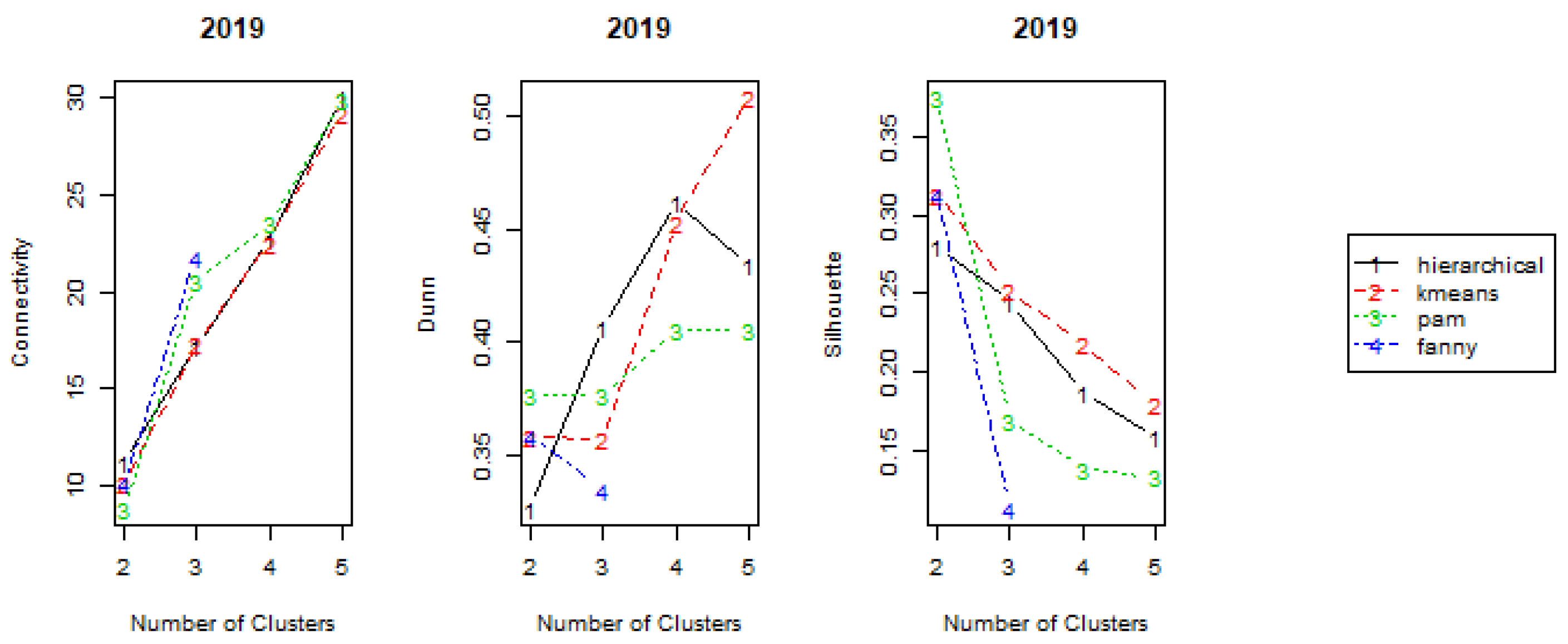
In order to determine the best number of clusters, internal validation measures were computed for all of the years and for hierarchical, pam, kmeans and fanny methods, as illustrated in Figure 3 (for the year 2019) and summarized in Table 1.
Figure 3.
Clusters’ internal validation measures for the year 2019.

Table 1.
Optimal cluster number (k) and method for internal measures.
The connectivity measure, Equation (7), varies between 0 and ∞ and should be minimized. Thus, looking at Figure 3 and Table 1, the optimal score for this measure, and for the year 2019, is obtained using the pam method and clusters. Observing the results for all the years, for most, the optimal connectivity value is found for and for the hierarchical method. The Dunn index, Equation (8), presents values between 0 and ∞ and should be maximized. It can be observed in Figure 3 and Table 1, that the best values of this measure are obtained for larger number of clusters. Silhouette Width, Equation (9), has values between and 1 and should be maximized. This is achieved mostly when clusters are considered and by using the hierarchical method.
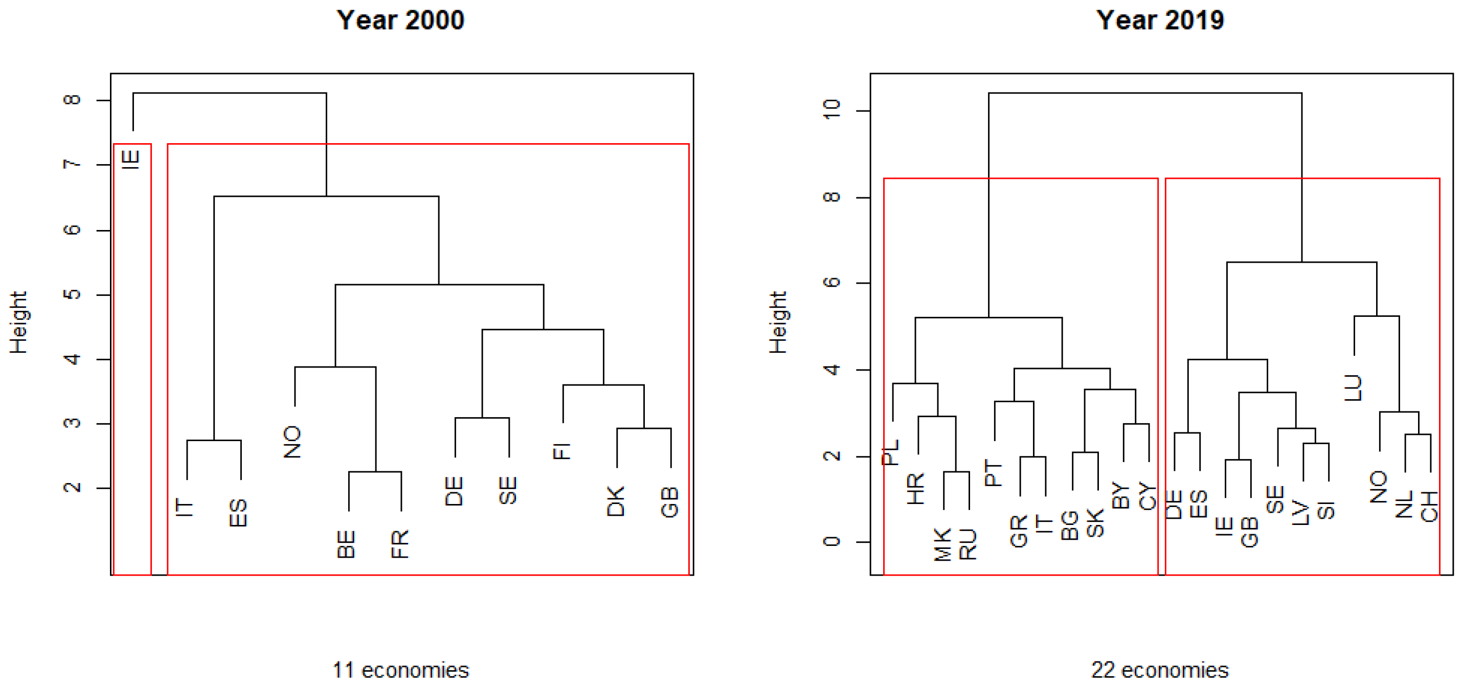
Table 2 shows that the optimal validation measures are obtained mostly for two clusters and for hierarchical methods. Furthermore, observing the dendrograms in Figure 4 for the years 2000 and 2009, and considering the cutting line at height = 7, the same conclusion is reached.
Table 2.
Clusters of European Economies from 2000 until 2019.

Figure 4.
Dendrograms for the years 2000 and 2019.
The software R, version 3.4.0, was used, and clusters were considered, as suggested in Table 1. The agglomeration of countries obtained for each year is presented in Table 2. For each year, the average of all the EFCs is shown in brackets for all countries (first and fourth columns), countries in Cluster 1 (second and fifth columns) and those in Cluster 2 (third and sixth columns). Note that Cluster 1 has an average below the global average and Cluster 2 has an average above the global average.
Analyzing the results inn Table 2, apart from Italy (IT) and Slovakia (SK), which remain in cluster 1, and Ireland (IE), Iceland (IS), Netherlands (NL) and Switzerland (CH), which maintain the allocation to cluster 2 throughout the two decades, the remaining countries’ allocations vary between the two clusters.
The agglomerations of the economies present different numbers of economies and also somewhat different averages and variability. Table 3 shows, for each year, the number of economies in each cluster and for all of the economies. This table also shows the average, standard deviation and coefficient of variation (CV) in %, of the average of the 12 EFCs. The average of the EFCs for all economies varies from 2.67 in 2010 to 2.92 in 2000, while larger variability is observed in 2015 (CV = 12.8%). Since 2009, when the number of economies started to significantly increase, the CV has been larger than 9.5%, reflecting the diversity of the economies participating in the survey. When analyzing each of the clusters, it can be seen that for Cluster 1, the lowest average was 2.37, observed in 2015, and the maximum was 2.88 in 2000. For Cluster 2, the minimum average was 2.78, observed in 2004, and the maximum was 3.4 in 2016. In 2016, only three of the 25 economies (i.e., 12%) were agglomerated in Cluster 2, while the other 22 economies were in Cluster 1, which had a CV of 8.8%, the largest observed in Cluster 1. In 2011 and 2011, Cluster 2 agglomerated only 9% and 14%, respectively, of the economies, leading to large averages—3.24 and 3.18, respectively.
Table 3.
Characterization of the clusters in Table 2.
Some particular cases that are worthy of discussion are as follows: Denmark (DK), which was allocated to the cluster with the lowest average only in 2000, while for the other 11 years for which there are data, it was always in Cluster 2. In fact, for 2000 as well as for 2011, 2013 and 2016, the economies allocated to Cluster 1 represent more than 85% of the economies for which there were data. This could explain why economies such as Germany (DE), Finland (FI), France (FR) Belgium (BE) and the United Kingdom (GB), which for the majority of the years were allocated to Cluster 2, were in most cases in 2000, 2011, 2013 and 2016 allocated to the cluster with the lowest average EFCs. Other countries, such as Portugal (PT), Greece (GR) and Spain (ES)m present more variability in the allocation to the two clusters.
To understand the pattern and exemplify differences in the cluster agglomeration over the years, we compared the allocations of the top European Economies with the best three and the three worst total early-stage entrepreneurial activity (TEA) values. TEA is a GEM indicator that represents the percentage of the 18–64-year-old population who are either a nascent entrepreneur or owner-manager of a new business.
Italy (TEA = 2.79), Poland (TEA = 5.39) and Belarus (TEA = 3.78) are the three countries with lower TEA values, and, in fact, Italy remains in Cluster 1 throughout the two decades, Poland, besides being allocated to Cluster 2 in 2015, is allocated to Cluster 1 in the remaining years. Belarus has only information in 2019, and it is allocated to Cluster 1, as expected.
On the other hand, the allocation of Latvia, which registers a higher TEA value for 2019 (TEA = 15.43), changes between Cluster 1 and Cluster 2, throughout the years. Slovakia, with the second-highest TEA value (TEA = 13.33), contrary to what was excepted, maintains its allocation to Cluster 1 in all years with information. Portugal (TEA = 12.89), the country with the third-highest TEA value, also presents differences in its allocation between Cluster 1 and cluster 2 throughout the years.
The obtained results indicate the need to consider annual and intra-country dynamics in studies on the topic of entrepreneurship, especially if they analyze data from GEM. Most studies (for example, the recent study of [2,11]) perform cross-sectional studies combining information from GEM with group economies. However, neglecting to consider a longitudinal dynamic may result in biased results.
4. Conclusions
In order to understand the dynamics of the European entrepreneurial framework conditions over the last two decades, cluster analysis was used to group the countries in homogeneous groups based on the EFCs experts’ perceptions during the period of 2000–2019.
The cluster analysis revealed that there are significant differences between the clusters obtained over the years and also that the distribution of the countries in each cluster considerably varies.
This study contributes to the existing literature in the sense that it clarifies the existence of a dynamic, entrepreneurial behavior of economies regarding entrepreneurial framework conditions, which should be considered in future works.
In the future, as a result of the differences encountered in countries’ agglomerations through time, a longitudinal clustering approach will be performed to compare results instead of the desegregated cross-sectional approach for each year. Furthermore, we intend to analyze the impact of the EFCs on entrepreneurship intentions and on total early-stage entrepreneurial activity (TEA) in Europe, making use of dynamic longitudinal models, in particular the system GMM procedure, to capture the intra-year and intra-country variability.
Author Contributions
This work was conducted by the three authors in collaboration through joint and distributed tasks. Joint tasks included conceptualization, writing—original draft preparation and writing—review and editing. Major contribution in software implementation, validation and visualization was given by E.C.e.S., A.B. mostly contributed with state-of-the-art investigations, formal analysis of the results and the finalization of the conclusions. A.C. defined the methodology, collected the resources and contributed to the interpretation and organization of the paper. All authors have read and agreed to the published version of the manuscript.
Funding
This work has been supported by national funds from FCT—Fundação para a Ciência e Tecnologia through project UIDB/04728/2020.
Institutional Review Board Statement
Not applicable.
Informed Consent Statement
Not applicable.
Data Availability Statement
Data used in this work is available on the GEM project website at https://www.gemconsortium.org/data and accessed 29 June 2020.
Conflicts of Interest
The authors declare no conflict of interest.
Abbreviations
The following abbreviations are used in this manuscript:
| APS | adult population survey |
| EDL | economic development level |
| EFCs | Entrepreneurial Framework Conditions |
| GEM | Global Entrepreneurship Monitor |
| NES | national expert survey |
| TEA | total early-stage entrepreneurial activity |
Appendix A
Table A1.
Description of Entrepreneurial Framework Conditions (EFCs). Source: [11].
Table A1.
Description of Entrepreneurial Framework Conditions (EFCs). Source: [11].
| EFC | Description | Indicator |
|---|---|---|
| 1 | The availability of financial resources—equity and debt—for small and medium enterprises (SMEs) (including grants and subsidies) | Financing for entrepreneurs |
| 2 | The extent to which public policies support entrepreneurship—entrepreneurship as a relevant economic issue | Governmental support and policies |
| 3 | The extent to which public policies support entrepreneurship—taxes or regulations are either size neutral or encourage new and SMEs | Taxes and bureaucracy |
| 4 | The presence and quality of programs directly assisting SMEs at all levels of government (national, regional, municipal) | Governmental programs |
| 5 | The extent to which training in creating or managing SMEs is incorporated within the education and training system at primary and secondary levels | Basic school entrepreneurial education and training |
| 6 | The extent to which training in creating or managing SMEs is incorporated within the education and training system in higher education, such as vocational education, college, business schools, etc. | Post-school entrepreneurial education and training |
| 7 | The extent to which national research and development will lead to new commercial opportunities and is available to SMEs | R&D transfer |
| 8 | The presence of property rights, commercial, accounting and other legal and assessment services and institutions that support or promote SMEs | Commercial and professional infrastructure |
| 9 | The level of change in markets from year to year | Internal market dynamics |
| 10 | The extent to which new firms are free to enter existing markets | Internal market openness |
| 11 | Ease of access to physical resources—communication, utilities, transportation, land or space—at a price that does not discriminate against SMEs | Physical and services infrastructure |
| 12 | The extent to which social and cultural norms encourage or allow actions leading to new business methods or activities that can potentially increase personal wealth and income | Cultural and social norms |
References
- Fernandes, A.J.; Ferreira, J.J. Entrepreneurial ecosystems and networks: A literature review and research agenda. Rev. Manag. Sci. 2021, 1–59. [Google Scholar] [CrossRef]
- Farinha, L.; Lopes, J.; Bagchi-Sen, S.; Sebastião, J.R.; Oliveira, J. Entrepreneurial dynamics and government policies to boost entrepreneurship performance. Socio Econ. Plan. Sci. 2020, 72, 100950. [Google Scholar] [CrossRef]
- De Brito, S.; Leitão, J. Mapping and defining entrepreneurial ecosystems: A systematic literature review. Knowl. Manag. Res. Pract. 2020, 19, 1–22. [Google Scholar] [CrossRef]
- Herrington, M.; Kew, P.K. Global Entrepreneurship Monitor: 2016/17 Global Report; Technical Report; Global Entrepreneurship Research Association (GERA): London, UK, 2017. [Google Scholar]
- Kelley, D.; Bosma, N.; Amorós, J.E. Global Entrepreneurship Monitor 2010 Global Report; Technical Report; Global Entrepreneurship Research Association (GERA): London, UK, 2011. [Google Scholar]
- Pilar, M.D.F.; Marques, M.; Correia, A. New and growing firms entrepreneurs’ perceptions and their discriminant power in edl countries. Glob. Bus. Econ. Rev. 2018, 21, 474–499. [Google Scholar] [CrossRef]
- Braga, V.; Queirós, M.; Correia, A.; Braga, A. High-Growth Business Creation and Management: A Multivariate Quantitative Approach Using GEM Data. J. Knowl. Econ. 2017, 9, 424–445. [Google Scholar] [CrossRef]
- Correia, A.; Costa e Silva, E.; Lopes, I.C.; Braga, A.; Braga, V. Experts’ perceptions on the entrepreneurial framework conditions. In AIP Conference Proceedings; AIP Publishing: New York, NY, USA, 2017; Volume 1906, p. 110004. [Google Scholar]
- Autio, E.; Kenney, M.; Mustar, P.; Siegel, D.; Wright, M. Entrepreneurial innovation: The importance of context. Res. Policy 2014, 43, 1097–1108. [Google Scholar] [CrossRef]
- Singer, S.; Herrington, M.; Menipaz, E. Global Entrepreneurship Monitor: Global Report 2017/18; Technical Report; Global Entrepreneurship Research Association (GERA): London, UK, 2018. [Google Scholar]
- Costa e Silva, E.; Correia, A.; Duarte, F. How Portuguese experts’ perceptions on the entrepreneurial framework conditions have changed over the years: A benchmarking analysis. In AIP Conference Proceedings; AIP Publishing LLC: New York, NY, USA, 2018; Volume 2040, p. 110005. [Google Scholar]
- Sokal, R.R. The principles and practice of numerical taxonomy. Taxon 1963, 12, 190–199. [Google Scholar] [CrossRef]
- Driver, H.E. Survey of numerical classification in anthropology. In The Use of Computers in Anthropology; De Gruyter Mouton: Berlin, Germany, 2011; pp. 301–344. [Google Scholar]
- Johnson, M.E. Multivariate Statistical Simulation: A Guide to Selecting and Generating Continuous Multivariate Distributions; John Wiley & Sons: Hoboken, NJ, USA, 1987; Volume 192. [Google Scholar]
- Walter, G.A.; Barney, J.B. Management objectives in Mergers and Acquisitions. Strateg. Manag. J. II(I) 1990, 11, 79–86. [Google Scholar] [CrossRef]
- Doyle, P.; Saunders, J. Market segmentation and positioning in specialized industrial markets. J. Mark. 1985, 49, 24–32. [Google Scholar] [CrossRef]
- Green, P.E.; Schaffer, C.; Patterson, K. A reduced space approach to the clustering of categorical data in market segmentation. J. Mark. 1991, 55, 20–31. [Google Scholar] [CrossRef]
- Reis, E. Estatística Multivariada Aplicada, 2nd ed.; Edições Sílabo: Lisboa, Portugal, 2001; ISBN 972-618-247-6. [Google Scholar]
- Aldenderfer, M.S.; Blashfield, R.K. Cluster analysis software and the literature on clustering. In Cluster Analysis; SAGE Publications Inc.: Thousand Oaks, CA, USA, 1984; pp. 75–81. [Google Scholar] [CrossRef]
- Ward, J.H., Jr. Hierarchical grouping to optimize an objective function. J. Am. Stat. Assoc. 1963, 58, 236–244. [Google Scholar] [CrossRef]
- Handl, J.; Knowles, J.; Kell, D.B. Computational cluster validation in post-genomic data analysis. Bioinformatics 2005, 21, 3201–3212. [Google Scholar] [CrossRef] [PubMed] [Green Version]
- Dunn, J.C. Well-separated clusters and optimal fuzzy partitions. J. Cybern. 1974, 4, 95–104. [Google Scholar] [CrossRef]
- Rousseeuw, P.J. Silhouettes: A graphical aid to the interpretation and validation of cluster analysis. J. Comput. Appl. Math. 1987, 20, 53–65. [Google Scholar] [CrossRef] [Green Version]
- Brock, G.; Pihur, V.; Datta, S.; Datta, S. clValid, an R package for cluster validation. J. Stat. Softw. 2008, 5, 1–22. [Google Scholar] [CrossRef] [Green Version]
- Bezdek, J.C.; Keller, J.; Krisnapuram, R.; Pal, N. Fuzzy Models and Algorithms for Pattern Recognition and Image Processing; Springer Science & Business Media: Berlin, Germany, 1999; Volume 4. [Google Scholar]
- Scitovski, R.; Sabo, K.; Martínez Álvarez, F.; Ungar, S. Cluster Analysis and Applications; Springer International Publishing: Berlin, Germany, 2021. [Google Scholar]
- Theodoridis, S.; Koutroumbas, K. Pattern Recognition, 4th ed.; Academic Press: Cambridge, MA, USA, 2009. [Google Scholar]
- Vendramin, L.; Campello, R.J.; Hruschka, E.R. On the comparison of relative clustering validity criteria. In Proceedings of the 2009 SIAM International Conference on Data Mining, SIAM, Sparks, NV, USA, 30 April–2 May 2009; pp. 733–744. [Google Scholar]
- Gajawada, S.; Toshniwal, D. Hybrid cluster validation techniques. In Advances in Computer Science, Engineering & Applications; Springer: Berlin, Germany, 2012; pp. 267–273. [Google Scholar]
Publisher’s Note: MDPI stays neutral with regard to jurisdictional claims in published maps and institutional affiliations. |
© 2021 by the authors. Licensee MDPI, Basel, Switzerland. This article is an open access article distributed under the terms and conditions of the Creative Commons Attribution (CC BY) license (https://creativecommons.org/licenses/by/4.0/).