Article

Modeling and Forecasting of COVID-19 Spreading by Delayed Stochastic Differential Equations

1
Laboratory of Analysis, Modeling and Simulation (LAMS), Faculty of Sciences Ben M’sik, Hassan II University of Casablanca, Sidi Othman, P.B. 7955 Casablanca, Morocco
2
Center for Research and Development in Mathematics and Applications (CIDMA), Department of Mathematics, University of Aveiro, 3810-193 Aveiro, Portugal
*
Author to whom correspondence should be addressed.
Axioms 2021, 10(1), 18; https://doi.org/10.3390/axioms10010018
Submission received: 3 December 2020 / Revised: 25 January 2021 / Accepted: 25 January 2021 / Published: 7 February 2021
(This article belongs to the Special Issue Axioms on Advanced Differential Equations for Mathematical Modeling)

Abstract

:
The novel coronavirus disease (COVID-19) pneumonia has posed a great threat to the world recent months by causing many deaths and enormous economic damage worldwide. The first case of COVID-19 in Morocco was reported on 2 March 2020, and the number of reported cases has increased day by day. In this work, we extend the well-known SIR compartmental model to deterministic and stochastic time-delayed models in order to predict the epidemiological trend of COVID-19 in Morocco and to assess the potential role of multiple preventive measures and strategies imposed by Moroccan authorities. The main features of the work include the well-posedness of the models and conditions under which the COVID-19 may become extinct or persist in the population. Parameter values have been estimated from real data and numerical simulations are presented for forecasting the COVID-19 spreading as well as verification of theoretical results.

1. Introduction

Coronaviruses are a large family of viruses that cause illnesses, ranging from the common cold to more serious illnesses such as Middle Eastern Respiratory Syndrome (MERS-CoV) and Severe Acute Respiratory Syndrome (SARS-CoV). The new coronavirus COVID-19 corresponds to a new strain that has not previously been identified in humans. On 11 March 2020, COVID-19 was reclassified as a pandemic by the World Health Organization (WHO). The disease has spread rapidly from country to country, causing enormous economic damage and many deaths around the world, prompting governments to issue a dramatic decree, ordering the lockdown of entire countries.
Since the confirmation of the first case of COVID-19 in Morocco on 2 March 2020 in the city of Casablanca, numerous preventive measures and strategies to control the spread of diseases have been imposed by the Moroccan authorities. In addition, Morocco declared a health emergency during the period from 20 March to 20 April 2020 and gradually extended it until 10 June 2020 in order to control the spread of the disease. In this paper, we report the assessment of the evolution of COVID-19 outbreak in Morocco. Besides shedding light on the dynamics of the pandemic, the practical intent of our analysis is to provide officials with the tendency of COVID-19 spreading, as well as gauge the effects of preventives measures using mathematical tools. Several other papers developed mathematical models for COVID-19 for particular regions in the globe and particular intervals of time, e.g., in [1] a Susceptible–Infectious–Quarantined–Recovered (SIQR) model to the analysis of data from the Brazilian Department of Health, obtained from 26 February 2020 to 25 March 2020 is proposed to better understand the early evolution of COVID-19 in Brazil; in [2], a new COVID-19 epidemic model with media coverage and quarantine is constructed on the basis of the total confirmed new cases in the UK from 1 February 2020 to 23 March 2020; while in [3] SEIR modelling to forecast the COVID-19 outbreak in Algeria is carried out by using available data from 1 March to 10 April 2020.
Mathematical modeling, particularly in terms of differential equations, is a strong tool that attracts the attention of many scientists to study various problems arising from mechanics, biology, physics, and so on. For instance, in [4], a system of differential equations with density-dependent sublinear sensitivity and logistic source is proposed and blow up properties of solutions are investigated; paper [5] presents a mathematical model with application in civil engineering related to the equilibrium analysis of a membrane with rigid and cable boundaries; [6] studies nonnegative and classical solutions to porous medium problems; and [7] a two-dimensional boundary value problem under proper assumptions on the data. Herein, we will focus on the dynamic of COVID-19. Tang et al. [8] used a Susceptible–Exposed–Infectious–Recovered (SEIR) compartmental model to estimate the basic reproduction number of COVID-19 transmission, based on data of confirmed cases for the disease in mainland China. Wu et al. [9] provided an estimate of the size of the epidemic in Wuhan on the basis of the number of cases exported from Wuhan to cities outside mainland China by using a SEIR model. In [10], Kuniya applied the SEIR compartmental model for the prediction of the epidemic peak for COVID-19 in Japan, using real-time data from 15 January to 29 February, 2020. Fanelli and Piazza [11] analyzed and forecasted the COVID-19 spreading in China, Italy and France, by using a simple Susceptible–Infected–Recovered–Deaths (SIRD) model. A more elaborate model, which includes the transmissibility of super-spreader individuals, is proposed in Ndaïrou et al. [12]. The model we propose here is new and has completely different compartments: in the paper [12], they model susceptible, exposed, symptomatic and infectious, super-spreaders, infectious but asymptomatic, hospitalized, recovered and the fatality class, with the main contribution being the inclusion of super-spreader individuals; in contrast, here we consider susceptible individuals, symptomatic infected individuals, which have not yet been treated, the asymptomatic infected individuals who are infected but do not transmit the disease, patients diagnosed and under quarantine and subdivided into three categories—benign, severe and critical forms—recovered and dead individuals. Moreover, our model has delays, while the previous model [12] has no delays; our model is stochastic, while the previous model [12] is deterministic. In fact, all mentioned models are deterministic and neglect the effect of stochastic noises derived from environmental fluctuations. To the best of our knowledge, research works that predict the COVID-19 outbreak taking into account a stochastic component, are a rarity [13,14,15]. The novelty of our work is twofold: the extension of the models cited above to a more accurate model with time delay, suggested biologically in the first place; secondly, to combine between the deterministic and the stochastic approaches in order to well-describe reality. To do this, Section 2 deals with the formulation and the well-posedness of the models. Section 3 is devoted to the qualitative analysis of the proposed models. Parameters estimation and forecast of COVID-19 spreading in Morocco is presented in Section 4 and Section 5, respectively. The paper ends with discussion and conclusions, in Section 6.

2. Models Formulation and Well-Posedness

Based on the epidemiological feature of COVID-19 and the several strategies imposed by the government, with different degrees, to fight against this pandemic, we extend the classical SIR model to describe the transmission of COVID-19 in the Kingdom of Morocco. In particular, we divide the population into eight classes, denoted by S, I s , I a , F b , F g , F c , R and M, where S represents the susceptible individuals; I s the symptomatic infected individuals, which have not yet been treated; I a the asymptomatic infected individuals who are infected but do not transmit the disease; F b , F g and F c denote the patients diagnosed, supported by the Moroccan health system and under quarantine, and subdivided into three categories: benign, severe and critical forms, respectively. Finally, R and M are the recovered and fatality classes. This model satisfies the following assumptions:
(1)
all coefficients involved in the model are positive constants;
(2)
natural birth and death rate are not factors;
(3)
true asymptomatic patients will stay asymptomatic until recovery and do not spread the virus;
(4)
patients who are temporarily asymptomatic are included on symptomatic ones;
(5)
the second infection is not considered in the model;
(6)
the Moroccan health system is not overwhelmed.
According to the above assumptions and the actual strategies imposed by the Moroccan authorities, the spread of COVID-19 in the population is modeled by the following system of delayed differential equations (DDEs):
d S ( t ) d t = β ( 1 u ) S ( t ) I s ( t ) N , d I s ( t ) d t = β ϵ ( 1 u ) S ( t τ 1 ) I s ( t τ 1 ) N α I s ( t ) ( 1 α ) ( μ s + η s ) I s ( t ) , d I a ( t ) d t = β ( 1 ϵ ) ( 1 u ) S ( t τ 1 ) I s ( t τ 1 ) N η a I a ( t ) , d F b ( t ) d t = α γ b I s ( t τ 2 ) μ b + r b F b ( t ) , d F g ( t ) d t = α γ g I s ( t τ 2 ) μ g + r g F g ( t ) , d F c ( t ) d t = α γ c I s ( t τ 2 ) μ c + r c F c ( t ) , d R ( t ) d t = η s ( 1 α ) I s ( t τ 3 ) + η a I a ( t τ 3 ) + r b F b ( t τ 4 ) + r g F g ( t τ 4 ) + r c F c ( t τ 4 ) , d M ( t ) d t = μ s ( 1 α ) I s ( t τ 3 ) + μ b F b ( t τ 4 ) + μ g F g ( t τ 4 ) + μ c F c ( t τ 4 ) ,
where t R + , N represents the total population size and u [ 0 , 1 ] denotes the level of the preventive strategies on the susceptible population. The parameter β indicates the transmission rate and ϵ [ 0 , 1 ] is the proportion for the symptomatic individuals. The parameter α denotes the proportion of the diagnosed symptomatic infected population that moves to the three forms: F b , F g and F c , by the rates γ b , γ g and γ c , respectively. The mean recovery period of these forms are denoted by 1 / r b , 1 / r g and 1 / r c , respectively. The latter forms die also with the rates μ b , μ g and μ c , respectively. Asymptomatic infected population, which are not diagnosed, recover with rate η a and the symptomatic infected ones recover or die with rates η s and μ s , respectively. The time delays τ 1 , τ 2 , τ 3 and τ 4 denote the incubation period, the period of time needed before the charge by the health system, the time required before the death of individuals coming from the compartments I s , F b , F g , and F c , respectively. At each instant of time,
D ( t ) = : μ s ( 1 α ) I s ( t τ 3 ) + μ b F b ( t τ 4 ) + μ g F g ( t τ 4 ) + μ c F c ( t τ 4 ) = d M ( t ) d t
gives the number of new death due to the disease (cf. [12]).
Remark 1.
In system (1), delays occur at the entrances, when the actions of infection take charge or the actions by the health system begin, and not at exits. Let us see an example. A susceptible individual, after contact with an infected person at instant t, becomes himself infected at instant t + τ 1 . Suddenly, the compartment of the infected is fed at the instant t by the susceptible infected at the instant t τ 1 . The same operation occurs at the level of the other interactions between the compartments of the model.
Remark 2.
We assume that the compartment of symptomatic infected I s does not completely empty at any time t. For this reason, one has μ s + η s < 1 . Note also that the diagnosed symptomatic infected population is completely distributed into one of three possible forms: F b , F g and F c , respectively by the rates γ b , γ g and γ c . Then, γ b + γ g + γ c = 1 .
Remark 3.
Biologically, τ 3 = 21 days and τ 4 = 13.5 days are the time periods needed before dying, deriving from I s and the three forms F b , F g , F c , respectively. That is why we inserted these delays in the last equation of system (1).
Remark 4.
We consider only a short time period in comparison to the demographic time-frame. From a biological point of view, this means that we can assume that there is neither entry (recruitment rate) nor exit (natural mortality rate), and vital parameters can be neglected. Note also that in our model, the individuals that die due to the disease are included in the population. Therefore, the total population is here assumed to be constant, that is, N ( t ) N during the period under study. This assumption is also reinforced by the fact that the Moroccan authorities have closed geographic borders.
The initial conditions of system (1) are
S ( θ ) = φ 1 ( θ ) 0 , I s ( θ ) = φ 2 ( θ ) 0 , I a ( θ ) = φ 3 ( θ ) 0 , F b ( θ ) = φ 4 ( θ ) 0 , F g ( θ ) = φ 5 ( θ ) 0 , F c ( θ ) = φ 6 ( θ ) 0 , R ( θ ) = φ 7 ( θ ) 0 , M ( θ ) = φ 8 ( θ ) 0 , θ [ τ , 0 ] ,
where τ = max { τ 1 , τ 2 , τ 3 , τ 4 } . Let C = C ( [ τ , 0 ] , R 8 ) be the Banach space of continuous functions from the interval [ τ , 0 ] into R 8 equipped with the uniform topology. It follows from the theory of functional differential equations [16] that system (1) with initial conditions
( φ 1 , φ 2 , φ 3 , φ 4 , φ 5 , φ 6 , φ 7 , φ 8 ) C
has a unique solution. On the other hand, due to continuous fluctuation in the environment, the parameters of the system are actually not absolute constants and always fluctuate randomly around some average value. Hence, using delayed stochastic differential equations (DSDEs) to model the epidemic provide some additional degree of realism compared to their deterministic counterparts. The parameters β and α play an important role in controlling and preventing COVID-19 spreading and they are not completely known, but subject to some random environmental effects. We introduce randomness into system (1) by applying the technique of parameter perturbation, which has been used by many researchers (see, e.g., [17,18,19]). In agreement, we replace the parameters β and α by β β + σ 1 B ˙ 1 ( t ) and α α + σ 2 B 2 ˙ ( t ) , where B 1 ( t ) and B 2 ( t ) are independent standard Brownian motions defined on a complete probability space ( Ω , F , P ) with a filtration { F t } t 0 satisfying the usual conditions (i.e., it is increasing and right continuous while F 0 contains all P-null sets) and σ i represents the intensity of B i for i = 1 , 2 . Therefore, we obtain the following model governed by delayed stochastic differential equations:
d S ( t ) = β ( 1 u ) S ( t ) I s ( t ) N d t σ 1 ( 1 u ) S ( t ) I s ( t ) N d B 1 ( t ) , d I s ( t ) = β ϵ ( 1 u ) S ( t τ 1 ) I s ( t τ 1 ) N α I s ( t ) ( 1 α ) ( μ s + η s ) I s ( t ) d t + σ 1 ϵ ( 1 u ) S ( t τ 1 ) I s ( t τ 1 ) N d B 1 ( t ) + σ 2 ( μ s + η s 1 ) I s ( t ) d B 2 ( t ) , d I a ( t ) = β ( 1 ϵ ) ( 1 u ) S ( t τ 1 ) I s ( t τ 1 ) N η a I a ( t ) d ( t ) + σ 1 ( 1 ϵ ) ( 1 u ) S ( t τ 1 ) I s ( t τ 1 ) N d B 1 ( t ) , d F b ( t ) = ( α γ b I s ( t τ 2 ) μ b + r b F b ( t ) ) d t + σ 2 γ b I s ( t τ 2 ) d B 2 ( t ) , d F g ( t ) = ( α γ g I s ( t τ 2 ) μ g + r g F g ( t ) ) d t + σ 2 γ g I s ( t τ 2 ) d B 2 ( t ) , d F c ( t ) = ( α γ c I s ( t τ 2 ) μ c + r c F c ( t ) ) d t + σ 2 γ c I s ( t τ 2 ) d B 2 ( t ) , d R ( t ) = ( η s ( 1 α ) I s ( t τ 3 ) + η a I a ( t τ 3 ) + r b F b ( t τ 4 ) + r g F g ( t τ 4 ) + r c F c ( t τ 4 ) ) d t σ 2 η s I s ( t τ 3 ) d B 2 ( t ) , d M ( t ) = ( μ s ( 1 α ) I s ( t τ 3 ) + μ b F b ( t τ 4 ) + μ g F g ( t τ 4 ) + μ c F c ( t τ 4 ) ) d t σ 2 μ s I s ( t τ 3 ) d B 2 ( t ) ,
where the coefficients are locally Lipshitz with respect to all the variables, for all t R + .
Let us denote R + 8 = { ( x 1 , x 2 , x 3 , x 4 , x 5 , x 6 , x 7 , x 8 ) x i > 0 , i = 1 , 2 , , 8 } . We have the following result.
Theorem 1.
For any initial value satisfying condition (3), there is a unique solution
x ( t ) = ( S ( t ) , I s ( t ) , I a ( t ) , F b ( t ) , F g ( t ) , F c ( t ) , R ( t ) , M ( t ) )
to the COVID-19 stochastic model (4) that remains in R + 8 with a probability of one.
Proof. 
Since the coefficients of the stochastic differential equations with several delays (4) are locally Lipschitz continuous, it follows from [20] that for any square integrable initial value x ( 0 ) R + 8 , which is independent of the considered standard Brownian motion B, there exists a unique local solution x ( t ) on t [ 0 , τ e ) , where τ e is the explosion time. For showing that this solution is global, knowing that the linear growth condition is not verified, we need to prove that τ e = . Let k 0 > 0 be sufficiently large for 1 k 0 < x ( 0 ) < k 0 . For each integer k k 0 , we define the stopping time τ k = inf t [ 0 , τ e ) s . t . x i ( t ) 1 k , k for some i = 1 , 2 , 3 , where inf = . It is clear that τ k τ e . Let T > 0 be arbitrary. Define the twice differentiable function W on R + * 3 R + as follows:
W ( x ) = ( x 1 + x 2 + x 3 ) 2 + 1 x 1 + 1 x 2 + 1 x 3 .
By Itô’s formula, for any 0 t τ k T and k 1 , we have
d W ( x ( t ) ) = L W ( x ( t ) ) d t + ζ ( x ( t ) ) d B ( t ) ,
where ζ is a continuous functional defined on [ 0 , + ) × C ( [ τ , 0 ] , R 3 × 2 ) by
ζ ( x ( t ) ) = σ 1 ( 1 u ) S ( t ) I s ( t ) N 0 σ 1 ϵ ( 1 u ) S ( t τ 1 ) I s ( t τ 1 ) N σ 2 ( μ s + η s 1 ) I s ( t ) σ 1 ( 1 ϵ ) ( 1 u ) S ( t τ 1 ) I s ( t τ 1 ) N 0 ,
B ( t ) = ( B 1 ( t ) , B 2 ( t ) ) T with the superscript “ T ” representing transposition, and L is the differential operator of function W defined by
L W ( x ( t ) ) = 2 ( S ( t ) + I s ( t ) + I a ( t ) ) 1 S 2 ( t ) β ( 1 u ) S ( t ) I s ( t ) N   + 1 + 1 S 3 ( t ) σ 1 ( 1 u ) S ( t ) I s ( t ) N 2   + 2 ( S ( t ) + I s ( t ) + I a ( t ) ) 1 I s 2 ( t ) β ϵ ( 1 u ) S ( t τ 1 ) I s ( t τ 1 ) N α I s ( t ) ( 1 α ) ( μ s + η s ) I s ( t )   + 1 + 1 I s 3 ( t ) σ 1 ϵ ( 1 u ) S ( t τ 1 ) I s ( t τ 1 ) N 2 + σ 2 ( μ s + η s 1 ) I s ( t ) 2   + 2 ( S ( t ) + I s ( t ) + I a ( t ) ) 1 I a 2 ( t ) β ( 1 ϵ ) ( 1 u ) S ( t τ 1 ) I s ( t τ 1 ) N η a I a ( t )   + 1 + 1 I a 3 ( t ) σ 1 ( 1 ϵ ) ( 1 u ) S ( t τ 1 ) I s ( t τ 1 ) N 2 .
Thus,
L W ( x ( t ) ) β ( 1 u ) S ( t ) I s ( t ) N S 2 ( t ) + 1 + 1 S 3 ( t ) σ 1 ( 1 u ) S ( t ) I s ( t ) N 2 + 2 β ϵ ( 1 u ) S ( t ) + I s ( t ) + I a ( t ) S ( t τ 1 ) I s ( t τ 1 ) N + α + ( 1 α ) ( μ s + η s ) I s ( t ) + 1 + 1 I s 3 ( t ) σ 1 ϵ ( 1 u ) S ( t τ 1 ) I s ( t τ 1 ) N 2 + σ 2 ( μ s + η s 1 ) I s ( t ) 2 + 2 β ( 1 ϵ ) ( 1 u ) S ( t ) + I s ( t ) + I a ( t ) S ( t τ 1 ) I s ( t τ 1 ) N + η a I a ( t ) + 1 + 1 I a 3 ( t ) σ 1 ( 1 ϵ ) ( 1 u ) S ( t τ 1 ) I s ( t τ 1 ) N 2 .
We now apply the elementary inequality 2 x y x 2 + y 2 , valid for any x , y R , by firstly taking x = β ϵ ( 1 u ) and y = S ( t ) + I s ( t ) + I a ( t ) and, secondly, x = β ( 1 ϵ ) ( 1 u ) and y = S ( t ) + I s ( t ) + I a ( t ) . In this way, we easily increase the right-hand side of inequality (5) to obtain that
L W ( x ( t ) ) b 1 + ψ S ( t ) + I s ( t ) + I a ( t ) 2 + b 2 S ( t ) + b 3 I s ( t ) + b 4 I a ( t ) D ( 1 + W ( x ( t ) ) ) ,
where ψ , b 1 , b 2 , b 3 , and b 4 are positive constants and D = max ψ , b 1 , b 2 , b 3 , b 4 . By integrating both sides of equality
d W ( x ( t ) ) = L W ( x ( t ) ) d t + ζ ( x ( t ) ) d B ( t )
between t 0 and t τ k and acting the expectation, which eliminates the martingale part, we get
E ( W ( x ( t τ k ) ) = E ( W ( x 0 ) ) + E t 0 t τ k L W ( x ( s ) ) ) d s E ( W ( x 0 ) ) + E t 0 t τ k D ( 1 + W ( x ( s ) ) ) d s E ( W ( x 0 ) ) + D T + t 0 t τ k E W ( x ( s ) ) ) d s
and Gronwall’s inequality implies that
E ( W ( x ( t τ k ) ) ( E W ( x 0 ) + D T ) exp ( C T ) .
For ω { τ k T } , x i ( τ k ) equals k or 1 k for some i = 1 , 2 , 3 . Hence,
W ( x i ( τ k ) ) k 2 + 1 k 1 k 2 + k .
It follows that
( E W ( x 0 ) + D T ) exp ( C T ) E χ { τ k T } ( ω ) W ( x τ k ) k 2 + 1 k 1 k 2 + k P ( τ k T ) .
Letting k , we get P ( τ e T ) = 0 . Since T is arbitrary, we obtain P ( τ e = ) = 1 . By defining the stopping time τ ˜ k = inf t [ 0 , τ e ) s . t . x i ( t ) 1 k , k for some i = 4 , , 8 , and considering the twice differentiable function W ˜ on R + * 5 R + as
W ˜ ( x ) = i = 4 8 x i 2 + i = 4 8 1 x i ,
we deduce, with the same technique, that all the variables of the system are positive on [ 0 , ) . □

3. Qualitative Analysis of the Models

The basic reproduction number, as a measure for disease spread in a population, plays an important role in the course and control of an ongoing outbreak [21]. This number is defined as the expected number of secondary cases produced, in a completely susceptible population, by a typical infective individual. Note that the calculation of the basic reproduction number R 0 does not depend on the variables of the system but depends on its parameters. In addition, the R 0 of our model does not depend on the time delays. For this reason, we use the next-generation matrix approach outlined in [22] to compute R 0 . Precisely, the basic reproduction number R 0 of system (1) is given by
R 0 = ρ ( F V 1 ) = β ϵ ( 1 u ) ( 1 α ) ( η s + μ s ) + α ,
where ρ is the spectral radius of the next-generation matrix F V 1 with
F = β ϵ ( 1 u ) 0 0 0 and V = ( 1 α ) ( η s + μ s ) + α 0 0 η a .
Noting that the classes that are directly involved in the spread of disease are only I s , I a , F b , F g and F c , we can reduce the local stability of system (1) to the local stability of
d I s ( t ) d t = β ϵ ( 1 u ) S ( t τ 1 ) I s ( t τ 1 ) N α I s ( t ) ( 1 α ) ( μ s + η s ) I s ( t ) , d I a ( t ) d t = β ( 1 ϵ ) ( 1 u ) S ( t τ 1 ) I s ( t τ 1 ) N η a I a ( t ) , d F b ( t ) d t = α γ b I s ( t τ 2 ) μ b + r b F b ( t ) , d F g ( t ) d t = α γ g I s ( t τ 2 ) μ g + r g F g ( t ) , d F c ( t ) d t = α γ c I s ( t τ 2 ) μ c + r c F c ( t ) .
The other classes are uncoupled to the equations of system (1) and the total population size N is constant. Then, we can easily obtain the following analytical results:
S ( t ) = N I s ( t ) + I a ( t ) + F b ( t ) + F g ( t ) + F c ( t ) + R ( t ) + M ( t ) , R ( t ) = 0 t η s ( 1 α ) I s ( δ τ 3 ) + η a I a ( δ τ 3 ) + r b F b ( δ τ 4 ) + r g F g ( δ τ 4 ) + r c F c ( δ τ 4 ) d δ , M ( t ) = 0 t μ s ( 1 α ) I s ( δ τ 3 ) + μ a I a ( δ τ 3 ) + μ b F b ( δ τ 4 ) + μ g F g ( δ τ 4 ) + μ c F c ( δ τ 4 ) d δ .
Let E ¯ = ( I s ¯ , I a ¯ , F b ¯ , F g ¯ , F c ¯ ) be an arbitrary equilibrium, and consider into system (7), the following change of unknowns:
U 1 ( t ) = I s ( t ) I s ¯ , U 2 ( t ) = I a ( t ) I a ¯ , U 3 ( t ) = F b ( t ) F b ¯ , U 4 ( t ) = F g ( t ) F g ¯ and U 5 ( t ) = F c ( t ) F c ¯ .
By substituting U i ( t ) , i = 1 , 2 , , 5 , into system (7) and linearizing around the free equilibrium, we get a new system that is equivalent to
d X ( t ) d t = A X ( t ) + B X ( t τ 1 ) + C X ( t τ 2 ) ,
where X ( t ) = ( U 1 ( t ) , U 2 ( t ) , U 3 ( t ) , U 4 ( t ) , U 5 ( t ) ) T and A, B, C are the Jacobian matrix of (7) given by
A = α ( 1 α ) ( μ s + η s ) 0 0 0 0 0 η a 0 0 0 0 0 ( μ b + r b ) 0 0 0 0 0 ( μ g + r g ) 0 0 0 0 0 ( μ c + r c ) ,
B = β ϵ ( 1 u ) 0 0 0 0 β ( 1 ϵ ) ( 1 u ) 0 0 0 0 0 0 0 0 0 0 0 0 0 0 0 0 0 0 0 ,
and
C = 0 0 0 0 0 0 0 0 0 0 α γ b 0 0 0 0 α γ g 0 0 0 0 α γ c 0 0 0 0 .
The characteristic equation of system (7) is given by
P ( λ ) = ( λ a 1 ( R 0 e λ τ 1 1 ) ) ( λ + η a ) ( λ + ( μ b + r b ) ) ( λ + ( μ g + r g ) ) ( λ + ( μ c + r c ) ) ,
where
a 1 = α + ( 1 α ) ( μ s + η s ) .
Clearly, the characteristic Equation (10) has the roots λ 1 = η a , λ 2 = ( μ b + r b ) , λ 3 = ( μ g + r g ) , λ 4 = ( μ c + r c ) and the root of the equation
λ a 1 ( R 0 e λ τ 1 1 ) = 0 .
We suppose R e ( λ ) 0 . From (11), we get
R e ( λ ) = a 1 ( R 0 e R e ( λ ) τ 1 cos ( I m λ τ 1 ) 1 ) < 0 ,
if R 0 < 1 , which contradicts R e ( λ ) 0 . On the other hand, we show that (11) has a real positive root when R 0 > 1 . Indeed, we put
Φ ( λ ) = λ a 1 ( R 0 e λ τ 1 1 ) .
We have that Φ ( 0 ) = a 1 ( R 0 1 ) < 0 , lim λ + Φ ( λ ) = + and function Φ is continuous on ( 0 , + ) . Consequently, Φ has a positive root and the following result holds.
Theorem 2.
The disease free equilibrium of system (1), that is, ( N , 0 , 0 , 0 , 0 , 0 , 0 , 0 ) , is locally asymptotically stable if R 0 < 1 and unstable if R 0 > 1 .
Knowing the value of the deterministic threshold R 0 characterizes the dynamical behavior of system (1) and guarantees persistence or extinction of the disease. Similarly, now we characterize the dynamical behavior of system (4) by a sufficient condition for extinction of the disease.
Theorem 3.
Let x ( t ) = S ( t ) , I s ( t ) , I a ( t ) , F b ( t ) , F g ( t ) , F c ( t ) , R ( t ) , M ( t ) be the solution of the COVID-19 stochastic model (4) with initial value x ( 0 ) defined in (3). Assume that
σ 1 2 > β 2 2 ( α + ( 1 α ) ( μ s + η s ) ) .
Then,
lim sup t + ln I s ( t ) t < 0 .
Namely, I s ( t ) tends to zero exponentially almost surely, that is, the disease dies out with a probability of one.
Proof. 
Let
d ln I s ( t ) = 1 I s ( t ) β ϵ ( 1 u ) S ( t τ 1 ) I s ( t τ 1 ) N α I s ( t ) ( 1 α ) ( μ s + η s ) I s ( t ) 1 2 I s 2 ( t ) σ 1 β ϵ ( 1 u ) S ( t τ 1 ) I s ( t τ 1 ) N 2 + σ 2 ( μ s + η s 1 ) I s ( t ) 2 d t + σ 1 β ϵ ( 1 u ) S ( t τ 1 ) I s ( t τ 1 ) N I s ( t ) d B 1 ( t ) + σ 2 ( μ s + η s 1 ) d B 2 ( t ) .
To simplify, we set
G ( t ) = ϵ ( 1 u ) S ( t τ 1 ) I s ( t τ 1 ) N , R 1 ( t ) = σ 1 β G ( t ) I s ( t ) , R 3 = σ 2 ( μ s + η s 1 ) , H = α ( 1 α ) ( μ s + η s ) .
Then, we get
d ln I s ( t ) = β G ( t ) I s ( t ) + H 1 2 σ 1 G ( t ) I s ( t ) 2 + R 3 2 d t + R 1 ( t ) d B 1 ( t ) + R 3 d B 2 ( t ) = σ 1 2 2 G ( t ) I s ( t ) 2 2 β σ 1 2 G ( t ) I s ( t ) + H R 3 2 2 d t + R 1 ( t ) d B 1 ( t ) + R 3 d B 2 ( t ) = σ 1 2 2 G ( t ) I s ( t ) β σ 1 2 2 β 2 σ 1 4 + H R 3 2 2 d t + R 1 ( t ) d B 1 ( t ) + R 3 d B 2 ( t ) β 2 2 σ 1 2 + H d t + R 1 ( t ) d B 1 ( t ) + R 3 d B 2 ( t ) .
Integrating both sides of the above inequality between 0 and t, one has
ln I s ( t ) t ln I s ( 0 ) t + β 2 2 σ 1 2 + H + M 1 ( t ) t + M 3 ( t ) t ,
where
M 1 ( t ) = 0 t R 1 ( s ) d B 1 ( s ) and M 3 ( t ) = 0 t R 3 d B 2 ( s ) .
We have
< M 1 , M 1 > t = 0 t σ 1 2 ϵ 2 ( 1 u ) 2 S ( s τ 1 ) 2 I s ( s τ 1 ) 2 N 2 I s 2 ( s ) d s 0 t σ 1 2 ϵ 2 ( 1 u ) 2 N 4 N 2 1 I s 2 ( s ) d s 0 t σ 1 2 ϵ 2 ( 1 u ) 2 d s .
Then,
lim sup t < M 1 , M 1 > t t σ 1 2 ϵ 2 ( 1 u ) 2 < + .
From the large number theorem for martingales [23], we deduce that
lim t M 1 ( t ) t = 0 .
We also have
< M 3 , M 3 > t = 0 t σ 3 2 ( μ s + η s 1 ) 2 d s = σ 3 2 ( μ s + η s 1 ) 2 t .
Then,
lim sup t < M 3 , M 3 > t t σ 3 2 ( μ s + η s 1 ) < +
and
lim t M 3 ( t ) t = 0 .
Subsequently,
lim sup t + ln I s ( t ) t β 2 2 σ 1 2 α ( 1 α ) ( μ s + η s ) .
We conclude that if β 2 2 σ 1 2 α ( 1 α ) ( μ s + η s ) < 0 , then lim I ( t ) t = 0 . This completes the proof. □

4. Assessment of Parameters

Estimating the model parameters poses a big challenge because the COVID-19 situation changes rapidly and from one country to another. The parameters are likely to vary over time as new policies are introduced on a day-to-day basis. For this reason, in order to simulate the COVID-19 models (1) and (4), we consider some parameter values from the literature, while the remaining ones are estimated or fitted.
As the transmission rate β is unknown, we carry out the least-square method [10] to estimate this parameter, based on the actual official reported confirmed cases from 2 March to 20 March, 2020 [24]. Through this method, we estimated β as 0.4517 (95%CI, 0.4484–0.455). Since the life expectancy for symptomatic individuals is 21 days on average and the crude mortality ratio is between 3 % to 4 % [25], we estimated μ s = 0.01 / 21 per day and η s = 0.8 / 21 per day. Furthermore, since the hospitals are not yet saturated and the epidemic situation is under control, we assume that mortality comes mainly from critical forms with a percentage of 40 % for an average period of 13.5 days [25]. Then, we choose μ c = 0.4 / 13.5 per day and r c = 0.6 / 13.5 per day. According to [26], the proportion of asymptomatic individuals varies from 20.6 % to 39.9 % and of symptomatic individuals from 60.1 % and 79.4 % of the infected population. The progression rates γ b , γ g and γ c , from symptomatic infected individuals to the three forms, are assumed to be 80 % of diagnosed cases for benign form, 15 % of diagnosed cases for severe form, and 5 % of diagnosed cases for critical form, respectively [25]. The incubation period is estimated to be 5.5 days [27,28] while the time needed before hospitalization is to be 7.5 days [29,30,31]. Following a clinical observation related to the situation of COVID-19 in Morocco, an evolution of symptomatic individuals is estimated towards recovery or death after 21 days without any clinical intervention. In the case when clinical intervention is applied, we estimate the evolution of the critical forms towards recovery or death after 13.3 days. The rest of the parameter values are shown in Table 1.

5. Numerical Simulation of Moroccan COVID-19 Evolution

In this section, we present the forecasts of COVID-19 in Morocco related to different strategies implemented by Moroccan authorities.
Taking into account the four levels of measures attached to containment, the effectiveness level of the applied Moroccan preventive measures is estimated to be
u = 0.2 , on ( 2 March , 10 March ] ; 0.3 , on ( 10 March , 20 March ] ; 0.4 , on ( 20 March , 6 April ] ; 0.8 , after 6 April .
In Figure 1, we see that the plots and the clinical data are globally homogeneous.
In addition, the last daily reported cases in Morocco [32], confirm the biological tendency of our model. Thus, our models are efficient to describe the spread of COVID-19 in Morocco. However, we note that some clinical data are far from the values of the models due to certain foci that appeared in some large areas or at the level of certain industrial areas. We conclude also that the stochastic behavior of COVID-19 presents certain particularities contrary to the deterministic one, namely the magnitude of its peak is higher and the convergence to eradication is faster. On the other hand, the conditions in Theorems 2 and 3 are verified. More precisely, the basic reproduction number R 0 = 0.5230 is less than one from 12 May 2020 and σ 1 2 = 1.0609 > 1.0598 = β 2 2 ( α + ( 1 α ) ( μ s + η s ) ) , which means that the eradication of disease is ensured.
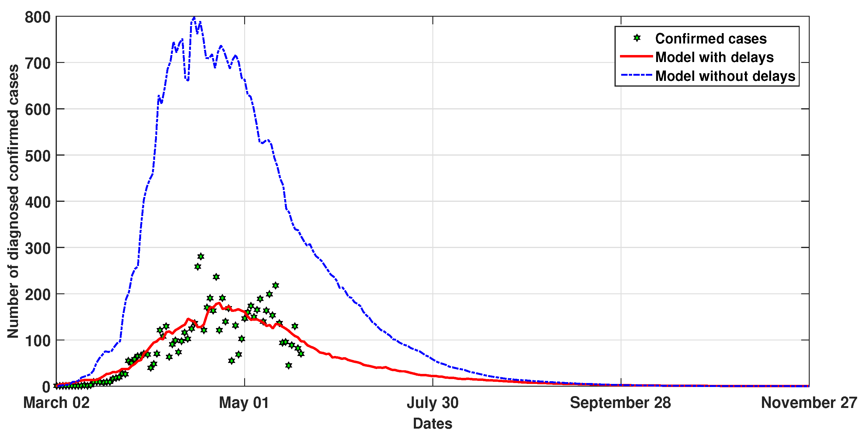
To prove the biological importance of delay parameters, we give the graphical results of Figure 2, which describe the evolution of diagnosed positive cases with and without delays.
We observe in Figure 2, a high impact of delays on the number of diagnosed positive cases, thereby the plot of model (4) without delays ( τ i = 0 , i = 1 , 2 , 3 , 4 ) is very different to that of the clinical data. Thus, we conclude that delays play an important role in the study of the dynamic behavior of COVID-19 worldwide, especially in Morocco, and allow us to better understand the reality.
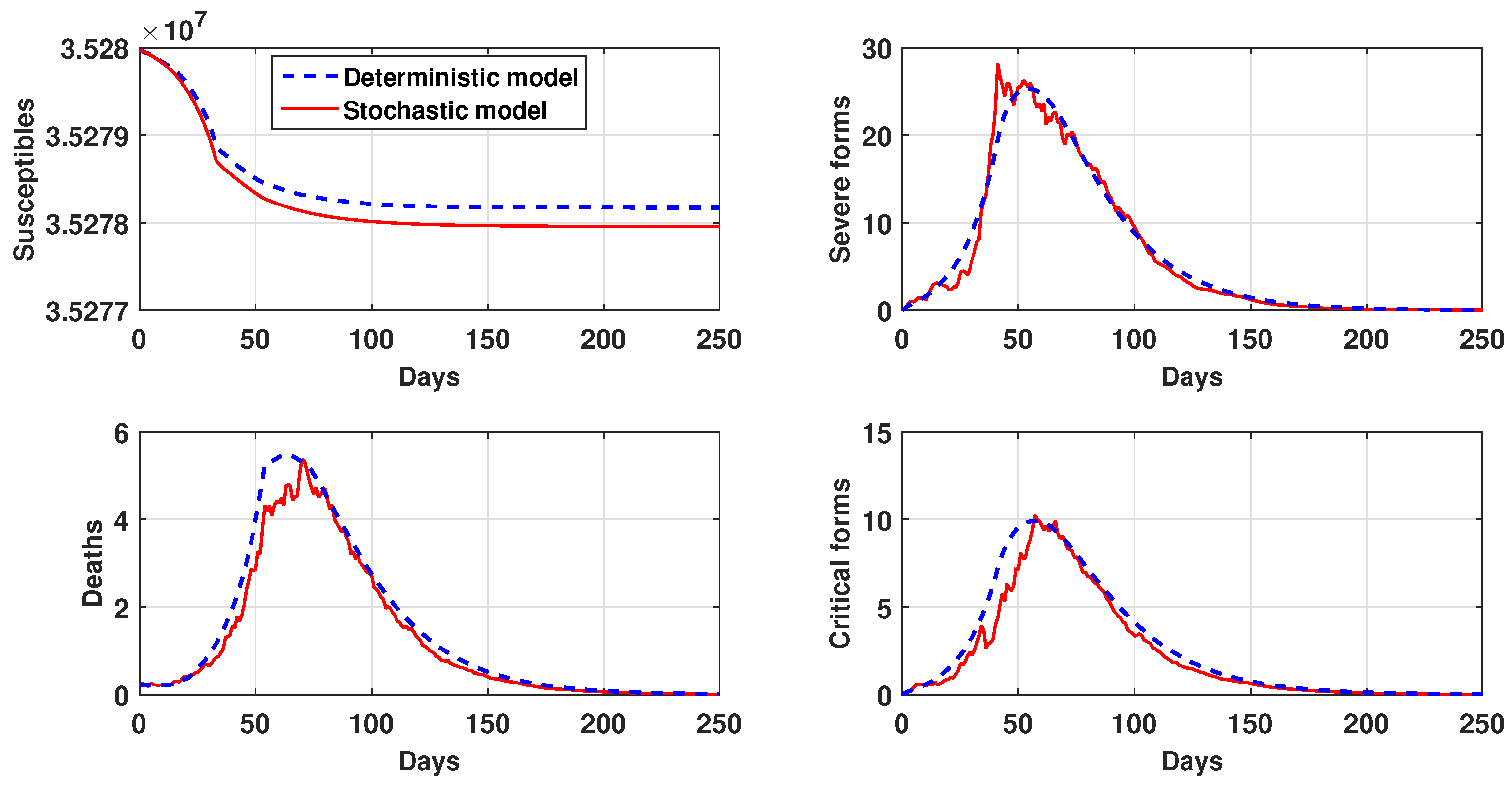
In Figure 3, we present the forecast of susceptible, severe forms of deaths and critical forms, from which we deduce that COVID-19 will not attack the total population.
In addition, the number of hospitalization beds or artificial respiration apparatus required can be estimated by the number of different clinical forms. Moreover, we see that the number of deaths given by the model is less than those declared in other countries [33], which shows that Morocco has avoided a dramatic epidemic situation by imposing the described strategies.
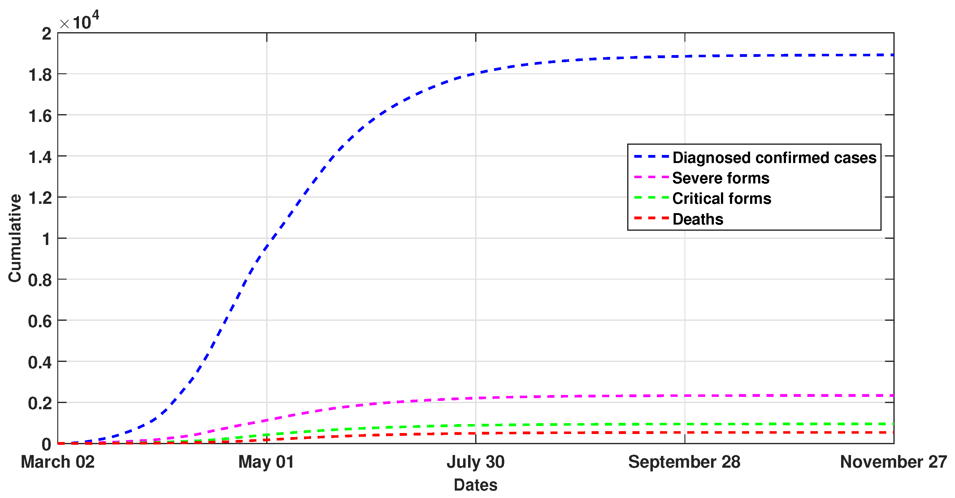
Finally, we present in Figure 4, the cumulative diagnosed cases, severe forms, deaths and critical forms 240 days from the start of the pandemic in Morocco. We summarize some important numbers in Table 2, which gives us some information about the future epidemic situation in Morocco.

6. Conclusions

In this study, we proposed a new deterministic model with delay and its corresponding stochastic model to describe the dynamic behavior of COVID-19 in Morocco. These models provide us with the evolution and prediction of important categories of individuals to be monitored, namely, the positive diagnosed cases, which can help to examine the efficiency of the measures implemented in Morocco, and the different developed forms, which can quantify the capacity of the public health system as well as the number of new deaths. Firstly, we have shown that our models are mathematically and biologically well posed by proving global existence and uniqueness of positive solutions. Secondly, the extinction of the disease was established. By analyzing the characteristic equation, we proved that if R 0 < 1 , then the disease free equilibrium of the deterministic model is locally asymptotically stable (Theorem 2). Based on the Lyapunov analysis method, a sufficient condition for the extinction was obtained in the stochastic case (Theorem 3). Thirdly, and since there is a substantial interest in estimating the parameters, we applied the least square method to determine the confidence interval of the transmission rate β as 0.4517 (95%CI, 0.4484–0.455). In addition, the rest of the parameters were either assumed, based on some daily observations, or taken from the available literature. Finally, some numerical simulations were performed to gather information in order to be able to fight against the propagation of the new coronavirus. In 12 May 2020, the basic reproduction number was less than one ( R 0 = 0.5230 ), which means that the epidemic was tending toward eradication, which is conditional on strict compliance with the implemented measures. Currently, the consequences of the measures taken against COVID-19 in Morocco encourage their maintenance to control the spread of the epidemic and quickly move towards extinction.
As future work, we intend to study the regional evolution of COVID-19 in Morocco.

Author Contributions

Conceptualization, M.M., A.B., H.Z., E.M.L., D.F.M.T. and N.Y.; Formal analysis, M.M., A.B., H.Z., E.M.L., D.F.M.T. and N.Y.; Investigation, M.M., A.B., H.Z., E.M.L., D.F.M.T. and N.Y.; Writing—original draft, M.M., A.B., H.Z., E.M.L., D.F.M.T. and N.Y.; Writing—review & editing, M.M., A.B., H.Z., E.M.L., D.F.M.T. and N.Y. All authors participated in the writing and reviewing of the paper. All authors have read and agreed to the published version of the manuscript.

Funding

H.Z. and D.F.M.T. were supported by FCT within project UIDB/04106/2020 (CIDMA).

Institutional Review Board Statement

Not applicable.

Informed Consent Statement

Not applicable.

Data Availability Statement

The data used in this study is available from the Government of Morocco, being given in Figure 1.

Acknowledgments

We would like to express our gratitude to the editor and the anonymous reviewers, for their constructive comments and suggestions, which helped us to enrich the paper.

Conflicts of Interest

The authors declare no conflict of interest. The funders had no role in the design of the study; in the collection, analyses, or interpretation of data; in the writing of the manuscript, or in the decision to publish the results.

References

  1. Crokidakis, N. Modeling the early evolution of the COVID-19 in Brazil: Results from a susceptible-infectious-quarantined-recovered (SIQR) model, Internat. J. Mod. Phys. C 2020, 31, 2050135. [Google Scholar] [CrossRef]
  2. Feng, L.-X.; Jing, S.-L.; Hu, S.-K.; Wang, D.-F.; Huo, H.-F. Modelling the effects of media coverage and quarantine on the COVID-19 infections in the UK. Math. Biosci. Eng. 2020, 17, 3618–3636. [Google Scholar] [CrossRef]
  3. Moussaoui, A.; Auger, P. Prediction of confinement effects on the number of Covid-19 outbreak in Algeria. Math. Model. Nat. Phenom. 2020, 15, 14. [Google Scholar] [CrossRef]
  4. Tanaka, Y.; Yokota, T. Blow-up in a parabolic-elliptic Keller-Segel system with density-dependent sublinear sensitivity and logistic source. Math. Methods Appl. Sci. 2020, 43, 7372–7396. [Google Scholar] [CrossRef]
  5. Viglialoro, G.; Murcia, J. A singular elliptic problem related to the membrane equilibrium equations. Int. J. Comput. Math. 2013, 90, 2185–2196. [Google Scholar] [CrossRef]
  6. Li, T.; Pintus, N.; Viglialoro, G. Properties of solutions to porous medium problems with different sources and boundary conditions. Z. Angew. Math. Phys. 2019, 70, 18. [Google Scholar] [CrossRef] [Green Version]
  7. Li, T.; Viglialoro, G. Analysis and explicit solvability of degenerate tensorial problems. Bound. Value Probl. 2018, 2018, 13. [Google Scholar] [CrossRef] [Green Version]
  8. Tang, B.; Wang, X.; Li, Q.; Bragazzi, N.L.; Tang, S.; Xiao, Y.; Wu, J. Estimation of the Transmission Risk of the 2019-nCoV and Its Implication for Public Health Interventions. J. Clin. Med. 2020, 9, 462. [Google Scholar] [CrossRef] [Green Version]
  9. Wu, J.T.; Leung, K.; Leung, G.M. Nowcasting and forecasting the potential domestic and international spread of the 2019-nCoV outbreak originating in Wuhan, China: A modelling study. Lancet 2020, 395, 689–697. [Google Scholar] [CrossRef] [Green Version]
  10. Kuniya, T. Prediction of the Epidemic Peak of Coronavirus Disease in Japan, 2020. J. Clin. Med. 2020, 9, 789. [Google Scholar] [CrossRef] [Green Version]
  11. Fanelli, D.; Piazza, F. Analysis and forecast of COVID-19 spreading in China, Italy and France. Chaos Solitons Fractals 2020, 134, 109761. [Google Scholar] [CrossRef] [PubMed]
  12. Ndaïrou, F.; Area, I.; Nieto, J.J.; Torres, D.F.M. Mathematical modeling of COVID-19 transmission dynamics with a case study of Wuhan. Chaos Solitons Fractals 2020, 135, 109846. [Google Scholar] [CrossRef] [PubMed]
  13. Simha, A.; Prasad, R.V.; Narayana, S. A simple stochastic SIR model for COVID 19 infection dynamics for Karnataka: Learning from Europe. arXiv 2020, arXiv:2003.11920. [Google Scholar]
  14. He, S.; Tang, S.; Rong, L. A discrete stochastic model of the COVID-19 outbreak: Forecast and control. Math. Biosci. Eng. 2020, 17, 2792–2804. [Google Scholar] [CrossRef]
  15. Bardina, X.; Ferrante, M.; Rovira, C. A stochastic epidemic model of COVID-19 disease. arXiv 2020, arXiv:2005.02859. [Google Scholar] [CrossRef]
  16. Hale, J.; Lunel, S.M.V. Introduction to Functional Differential Equations; Springer: New York, NY, USA, 1993. [Google Scholar]
  17. Mahrouf, M.; Hattaf, K.; Yousfi, N. Dynamics of a stochastic viral infection model with immune response. Math. Model. Nat. Phenom. 2017, 12, 15–32. [Google Scholar] [CrossRef]
  18. Hattaf, K.; Mahrouf, M.; Adnani, J.; Yousfi, N. Qualitative analysis of a stochastic epidemic model with specific functional response and temporary immunity. Phys. A Stat. Mech. Appl. 2018, 490, 591–600. [Google Scholar] [CrossRef]
  19. Dalal, N.; Greenhalgh, D.; Mao, X. A stochastic model of AIDS and condom use. J. Math. Anal. Appl. 2007, 325, 36–53. [Google Scholar] [CrossRef] [Green Version]
  20. Mao, X. Stochastic Differential Equations and Applications; Elsevier: Amsterdam, The Netherlands, 2007. [Google Scholar]
  21. Diekmann, O.; Heesterbeek, J.A.P.; Metz, J.A.J. On the definition and the computation of the basic reproduction ratio R0 in models for infectious diseases in heterogeneous populations. J. Math. Biol. 1990, 28, 365–382. [Google Scholar] [CrossRef] [Green Version]
  22. Driessche, P.V.; Watmough, J. Reproduction numbers and sub-threshold endemic equilibria for compartmental models of disease transmission. Math. Biosci. 2002, 180, 29–48. [Google Scholar] [CrossRef]
  23. Grai, A.; Greenhalgh, D.; Hu, L.; Mao, X.; Pan, J. A stochastic differential equations SIS epidemic model. SIAM J. Appl. Math. 2011, 71, 876–902. [Google Scholar] [CrossRef] [Green Version]
  24. Ministry of Health, Morocco. Department of Epidemiology and Disease Control. Available online: http://www.sante.gov.ma/Pages/Accueil.aspx (accessed on 30 May 2020).
  25. WHO. Coronavirus Disease 2019 (COVID-19); Situation Report 46, 6 March 2020; WHO: Geneva, Switzerland, 2020. [Google Scholar]
  26. Mizumoto, K.; Kagaya, K.; Zarebski, A.; Chowell, G. Estimating the asymptomatic proportion of coronavirus disease 2019 (COVID-19) cases on board the Diamond Princess cruise ship, Yokohama, Japan, 2020. Euro Surveill. 2020, 25, 2000180. [Google Scholar] [CrossRef] [PubMed] [Green Version]
  27. WHO. Coronavirus Disease 2019 (COVID-19); Situation Report 73, 2 April 2020; WHO: Geneva, Switzerland, 2020. [Google Scholar]
  28. Baum, S.G. COVID-19 Incubation Period: An Update. Available online: https://www.jwatch.org/na51083/2020/03/13/covid-19-incubation-period-update (accessed on 13 March 2020).
  29. Huang, C.; Wang, Y.; Li, X.; Ren, L.; Zhao, J.; Hu, Y.; Zhang, L.; Fan, G.; Xu, J.; Gu, X.; et al. Clinical features of patients infected with 2019 novel coronavirus in Wuhan, China. Lancet 2020, 395, 497–506. [Google Scholar] [CrossRef] [Green Version]
  30. Wang, D.; Hu, B.; Hu, C.; Zhu, F.; Liu, X.; Zhang, J.; Wang, B.; Xiang, H.; Cheng, Z.; Xiong, Y.; et al. Clinical Characteristics of 138 Hospitalized Patients with 2019 Novel Coronavirus-Infected Pneumonia in Wuhan, China. J. Am. Med. Assoc. 2020, 323, 1061–1069. [Google Scholar] [CrossRef] [PubMed]
  31. Haut Conseil de la Santé Publique. Avis Relatif aux Recommandations Thérapeutiques dans la Prise en Charge du COVID-19 (Complémentaire à l’avis du 5 mars 2020), 23 Mars 2020. Available online: https://splf.fr/wp-content/uploads/2020/03/HCSP-Avis-relatif-aux-recommandations-therapeutiques-dans-la-prise-en-charge-du-COVID-19-complementaire-a-avis-du-5-mars-2020-le23-03-20.pdf (accessed on 30 May 2020).
  32. Ministry of Health of Morocco. The Official Portal of Corona Virus in Morocco. Available online: https://www.sante.gov.ma/Pages/Accueil.aspx (accessed on 30 May 2020).
  33. COVID-19 Coronavirus Pandemic, View by Country. Available online: https://www.worldometers.info/coronavirus/#countries (accessed on 30 May 2020).
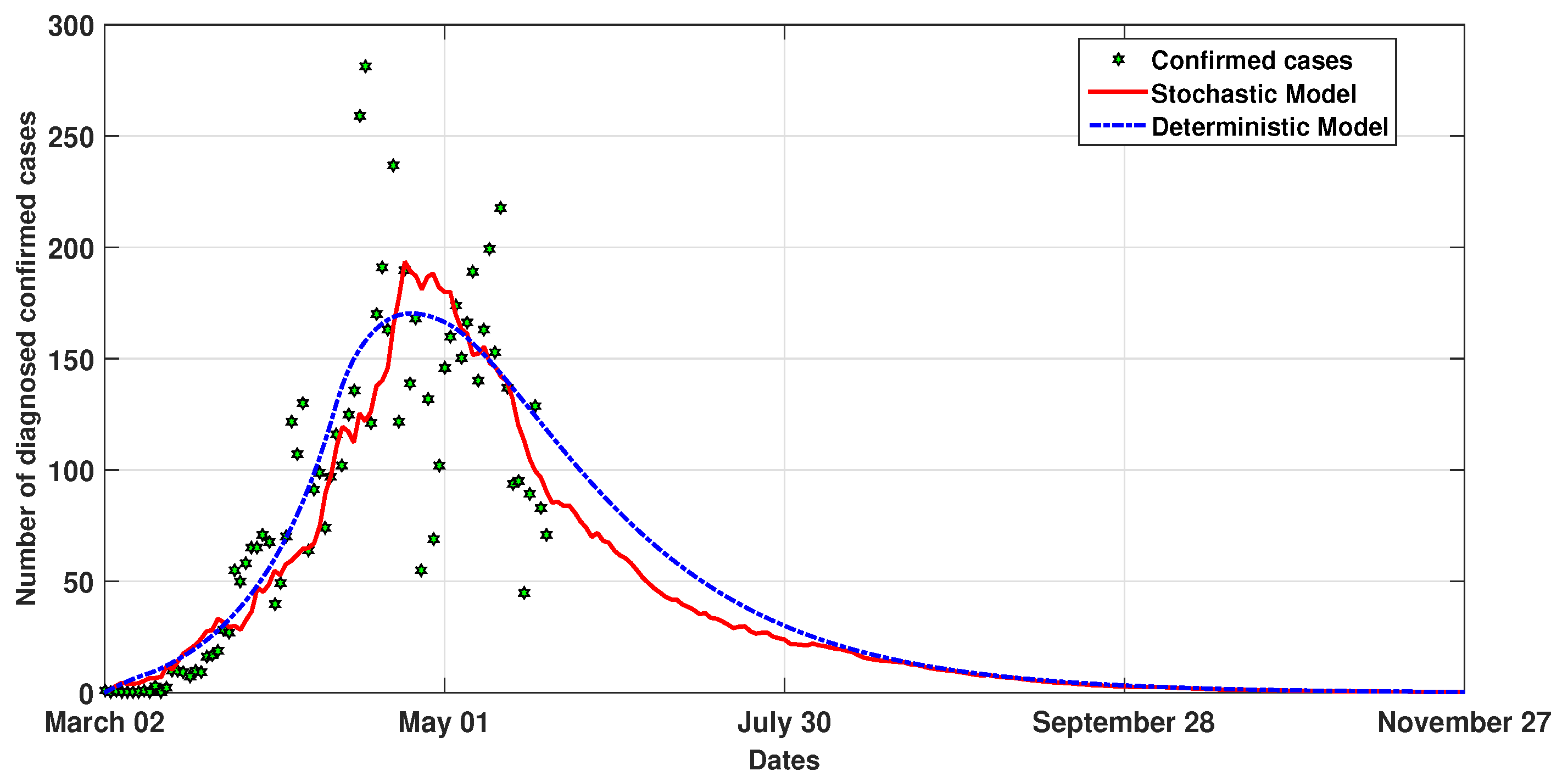
Figure 1. Comparison of the deterministic and the stochastic dynamical behavior with the daily reported cases of COVID-19 in Morocco.
Axioms 10 00018 g001
Figure 2. Effect of delays on the diagnosed confirmed cases.
Axioms 10 00018 g002
Figure 3. The evolution of susceptible, deaths, severe and critical forms from 2 March 2020.
Axioms 10 00018 g003
Figure 4. Cumulative diagnosed cases, severe forms, critical forms and deaths 240 days from the start of the COVID-19 pandemic in Morocco.
Axioms 10 00018 g004
Table 1. Parameter values of models (1) and (4).
ParameterValueSourceParameterValueSource
β 0.4517 Estimatedu[0–1]Varied
ϵ 0.794 [26] γ b 0.8 [25]
γ g 0.15 [25] γ c 0.05 [25]
α 0.06Assumed η a 1 / 21 Calculated
η s 0.8 / 21 Calculated μ s 0.01 / 21 Calculated
μ b 0Assumed μ g 0Assumed
μ c 0.4 / 13.5 Calculated r b 1 / 13.5 Calculated
r g 1 / 13.5 Calculated r c 0.6 / 13.5 Calculated
τ 1 5.5 [27,28] τ 2 7.5 [29,30,31]
τ 3 21Assumed τ 4 13.5 Assumed
σ 1 1.03 Calculated σ 2 0.1 Assumed
Table 2. Estimated peaks and cumulative of diagnosed cases, severe forms, critical forms and deaths.
CompartmentsPeakCumulative
DiagnosedAround 19018,890
Severe formsAround 282233
Critical formsAround 10997
DeathsAround 5468
Publisher’s Note: MDPI stays neutral with regard to jurisdictional claims in published maps and institutional affiliations.