Multivariate Simulation in Non-Stationary Domains: A Framework for Accurate Data Reproduction

Abstract

Accurate multivariate Gaussian simulation is critical for resource assessment and mine planning, especially in polymetallic deposits where strong trends, data bias, and multivariate outliers introduce complexity. In this scenario, standard workflows applied to non-stationary domains may result in undesirable data statistics reproduction, especially the multivariate relationships between variables. This study proposes an enhanced simulation framework that integrates data standardization, multivariate outlier detection, trend modeling and removal, and a dual application of the Projection Pursuit Multivariate Transform (PPMT). The approach is demonstrated within a high-grade mineralized breccia domain of the Peñasquito deposit, utilizing data from diamond core and reverse circulation (RC) drill holes, including Au, Ag, Pb, and Zn. Bias in RC data was corrected using data standardization, and multivariate outliers were identified through the application of a robust Mahalanobis distance. Trend modeling was performed using a moving window average and was removed using the Gaussian Mixture Model and Stepwise Conditional Transform. PPMT was applied both before and after trend modeling in order to improve decorrelation and simulation performance. Results show improved data reproduction through histograms, variograms, and complex relationships, as well as correlation coefficients. Cross-validation confirms reduced bias and improved accuracy. This research highlights the importance of treating multivariate outliers and applying PPMT both before and after trend modeling. The study demonstrates that applying PPMT twice is more effective for managing persistent non-stationary features, especially in high-grade domains.

1. Introduction

Mining operations rely on accurate orebody characterization and modeling for effective decision-making in resource assessment, process optimization, and environmental management. Multivariate simulation is used to quantify uncertainty that, in turn, enables risk-qualified decision-making. This is performed by generating multiple realizations that capture the correct variability [1] of the orebody under evaluation, resulting in more globally accurate results.

Geostatistical simulation assumes stationarity [2,3]; however, natural phenomena, especially mineral deposits, often exhibit trends (non-stationarity) in the data. These trends violate the assumption of stationarity, making geostatistical modeling more challenging [3]. Before performing a simulation, it is necessary to model and remove these trends. The Moving Window Average (MWA) method offers a flexible, data-driven approach to trend modeling by averaging nearby samples within a centered window [4]. This produces a smooth, large-scale deterministic trend surface that reflects the distribution of high- and low-grade areas. The conventional trend removal approach involves subtracting the trend surface from the observed data. Estimation or simulation is then performed on the residuals, followed by reintroducing the trends in the final results [5,6]. However, this has limitations in capturing the complex relationships between the residuals and trends. A more modern approach addresses these limitations by utilizing a Gaussian Mixture Model (GMM) and Stepwise Conditional Transform (SCT) to remove the dependency between the data and trend. Both the data and trend are transformed into Normal Score (NS) units. A GMM is then fitted to the collocated pairs to capture their joint distribution [6,7]. Using the GMM, SCT [8,9] is then applied, resulting in uncorrelated residuals with respect to the trend. While this modern approach overcomes many of the limitations, it still depends on subjective judgments when choosing the optimal trend model and fitting parameters.

In multivariate simulation, the residuals are decorrelated using linear and non-linear methods. This approach is less time-consuming than traditional co-simulation [10,11,12,13] because the variables are modeled individually. Various decorrelation methods have been used [14,15,16,17,18,19,20,21,22,23] for Gaussian simulations. Projection pursuit multivariate transform (PPMT) is widely used to decorrelate non-linear and complex relationships [20,24]. It transforms multivariate data into independent Gaussian components, enabling independent simulations. PPMT has generally been shown to deliver the most accurate results when compared with other methods.

Using real geological data presents numerous challenges that add to the complexity when performing simulations in complex deposits. One of the most common issues is data bias, particularly when samples are collected by different drilling methods [1], such as diamond drilling (DDH) versus reverse circulation (RC) drilling. In particular, RC drilling introduces bias due to contamination, loss of fines, sample recovery issues, and other sampling-related problems. While discarding RC data is not recommended, identifying and correcting this bias should be considered standard practice before performing estimation or simulation. Additionally, the presence of outliers in multivariate data challenges the accuracy of simulation results. Outliers are typically managed in a univariate context. This approach is insufficient for multivariate data, where remnant outliers can significantly distort variogram structures and compromise the effectiveness of trend models and decorrelation techniques, such as PPMT. In domains with strong trends, complex spatial patterns, and complex non-linear relationships, advanced methods of trend modeling and decorrelation may be insufficient to accurately simulate multivariate data. An appropriate simulation, for example, should accurately reproduce the variable distribution [25,26] through histograms, spatial continuity through variograms, and multivariate relationships through correlation matrices or scatter plots. Poor data reproduction often leads to misinterpretations, including biased results. Importantly, this can directly affect the accuracy of the resource model and mine planning decisions, which ultimately affect the economic viability of a given orebody.

This study proposes an enhanced multivariate simulation workflow designed for complex non-stationary domains. The methodology addresses four key issues: data bias, multivariate outliers, trend modeling, and decorrelation. This approach applies PPMT both before and after trend modeling, followed by Gaussian simulation. This double application of the PPMT was implemented to enhance data reproduction, including statistical distributions, correlation coefficients, and spatial continuity.

Accurate data statistics reproduction is one of the main objectives of geostatistical simulation. In contrast, poor reproduction of histograms can distort grade-tonnage relationships and result in misleading resource estimates. Inaccurate variogram reproduction can lead to a misrepresentation of the spatial extent and connectivity of geological features. Additionally, poor reproduction of multivariate relationships can negatively impact blending strategies, metallurgical recovery, and the overall mine plan for the deposit. The following proposed workflow addresses these challenges using a systematic approach for simulating multivariate data in geologically complex, non-stationary domains.

2. Proposed Methodology and Practical Application

Building on the outlined theoretical framework, this study explores the practical application of the proposed multivariate simulation workflow using a case study of a mineralized breccia domain within the Peñasquito mine.

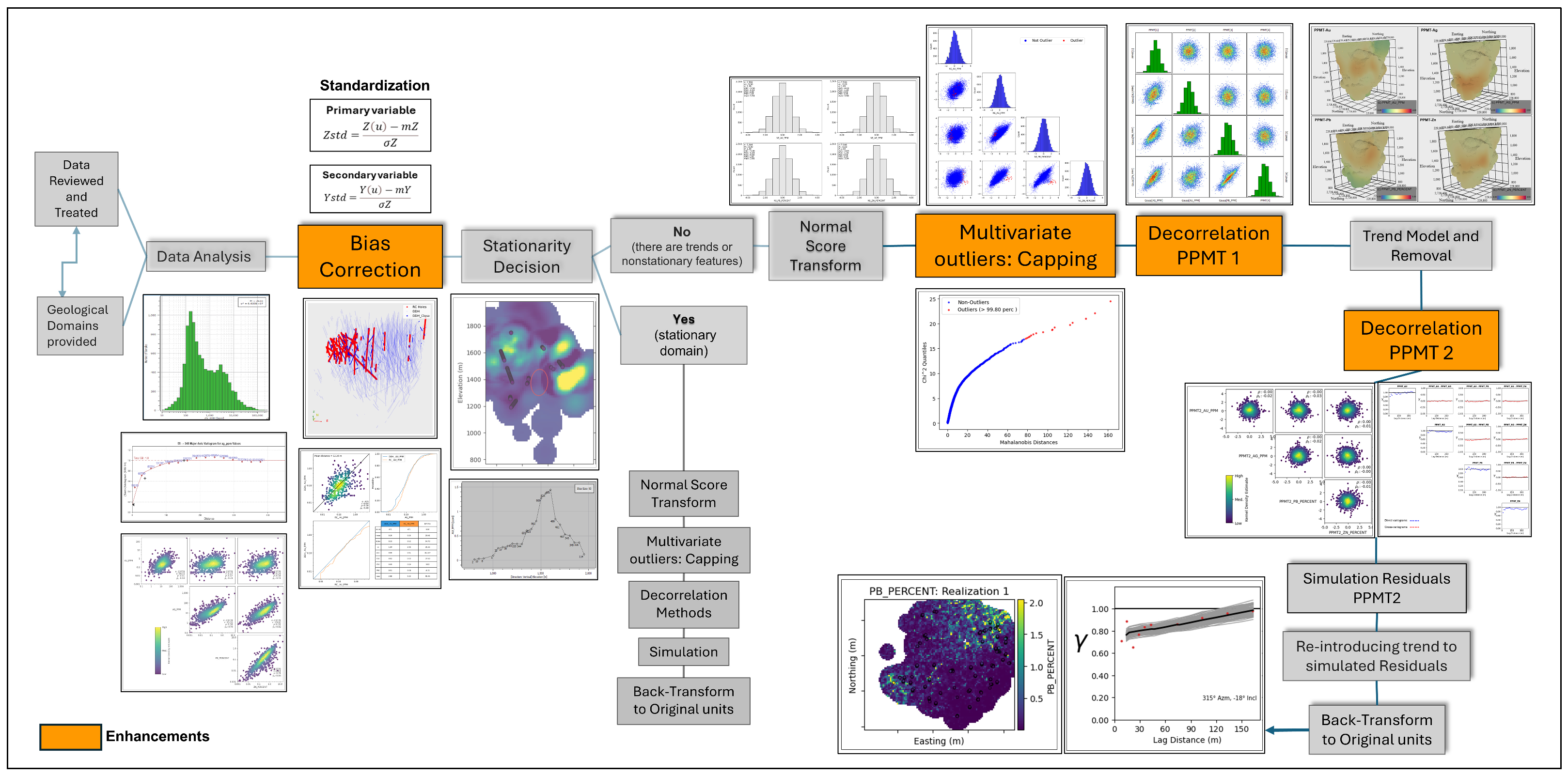
This study proposes a multivariate simulation workflow designed for modeling complex, non-stationary geological domains. The methodology addresses key challenges, including data bias from drilling methods, multivariate outliers, strong trends, and non-linear complex correlations between variables. The process begins with data standardization, where the bias in the variables under evaluation is addressed, along with the RC data correction process. In the multivariate outlier treatment stage, multivariate outliers are identified and evaluated using robust Mahalanobis distance. This is completed using standardized data that was previously capped (univariate capping). For trend modeling, the moving window average method is applied to model the trend, which is then removed using the GMM and SCT approaches. The PPMT method is applied both before and after trend modeling. Gaussian simulation is then performed on the PPMT2 residuals. The double application of PPMT is a key component of the proposed framework, which also addresses biases between drillhole types and treats multivariate outliers using the Mahalanobis distance. Explicitly managing outliers in a multivariate context is rarely performed in Gaussian simulation workflows. The motivation for applying PPMT twice is practical rather than theoretical. The first PPMT ensures variables are Gaussian and nearly independent before trend modeling. The second PPMT addresses any residual dependencies that were reintroduced during the trend modeling and removal. This approach allows more effective management of persistent non-stationary features compared to only NS transformation before trend modeling. Figure 1 illustrates a schematic flow diagram of the proposed workflow, which highlights enhancements shown in orange [27].

The dataset used in this study includes composited drill hole samples obtained from both the DDH and RC drilling methods. The multivariate simulation included Au, Ag, Pb, and Zn (homotopic data) using one representative domain as a proof of the concept. The primary, DDH, and secondary RC holes data are non-collocated, where the primary data are more abundant than the secondary data. Grade capping was performed in the univariate space to reduce the influence of extreme values. Declustering was then applied to correct sampling bias, ensuring that both densely and sparsely drilled areas were appropriately represented in this study. The details of the research data and deposit type are covered in the case study section. This study was primarily conducted using RMSP software (version 1.14.1), with additional use of Isatis.neo Mining software (version 2024.04.2).

2.1. Bias Detection and Correction

To evaluate and correct the systematic bias between primary (DDH) and secondary (RC) drilling data, a spatial pairing analysis was performed [28]. This approach involves matching nearby DDH and RC samples within a specified search distance range to assess relative differences. To apply the correction, the mean and standard deviation differences from the pairing analysis were used to infer adjusted DDH statistics. The secondary data $Y\left(u\right)$ were standardized by subtracting the mean ($mY)$ and dividing it by the standard deviation ($\sigma Y)$ as follows:

$$Ystd={\displaystyle \frac{Y\left(u\right)-mY}{\sigma Y}}$$

(1)

This results in a normalized dataset with a mean of zero and a standard deviation of one, using the standardization approach described by [1] in the context of cokriging. These standardized values were then transformed back to the original units using the following:

$$CorrectedRC=\left(Ystd\times Infer.DDHStd\right)+Infer.DDHmean$$

(2)

This correction was applied to all secondary samples prior to geostatistical analysis. By incorporating multiple data types, particularly in areas with limited sampling, the goal was to improve the data reproduction and overall accuracy of the simulation results.

2.2. Multivariate Outlier Detection

Multivariate outliers are observations that do not follow the overall pattern when multiple variables are analyzed together. Although univariate capping is commonly applied before grade modeling and variogram analysis, it is insufficient for detecting multivariate outliers when working with complex multivariate datasets. Identifying and managing these outliers should be standard practice in simulation workflows, as they can affect data analysis, variogram modeling, decorrelation, and simulation results. Multivariate outliers were identified using the Mahalanobis Distance method, which measures the distance of a point from the multivariate mean, simultaneously accounting for the covariance between variables [29]. Notably, this particular method is also sensitive to extreme values. Therefore, instead, the Robust Mahalanobis Distance (MCD) was used. This approach estimates the mean and covariance from the most central subset of data, yielding more stable results [30]. Prior to the calculation, the data were transformed to normal scores to ensure that no single variable dominated the distance calculation. Sensitivity analysis and cross-validation guided the capping strategy.

2.3. Trend Modeling and Removal

Gaussian simulation relies on the assumption of stationarity, but overall scale trends violate this assumption and challenge geostatistical modeling [3]. Trend modeling was applied to the normal score data. The Moving Window Average (MWA) method was used to fit a trend by centering a window on each grid location and assigning the weighted average of samples within that window [4,6]. The search strategy was defined based on the variogram anisotropy. The minimum number of samples included in the window and the scale factor for smoothing were selected based on the data density and anisotropy, following guidelines such as the square root of the anisotropy rule to mitigate directional effects [3]. This is critical for domains with strong anisotropy. All these parameters are included in the optimization using the TrendEstimator function [28], along with a review of the minimum number of composites to minimize trend residual correlation. The result is a smooth trend model that captures large-scale patterns without introducing overfitting or artifacts. The following step involves removing the dependency between the trend and the data as part of the trend removal step using a Trend Transformer function [28]. This approach fits a GMM to the paired data values and trends and then applies SCT to yield uncorrelated residuals. After the simulation, the trend was then reintroduced into the realizations.

2.4. Multivariate Decorrelation

In multivariate simulation, one important goal is to simulate multiple variables while preserving their relationships in the final results. Multivariate decorrelation was performed using PPMT. This technique was derived from Projection Pursuit Density Estimation (PPDE), a non-parametric method introduced by [31] in 1987. PPMT aims to find a linear combination of multivariate data that results in a Gaussian distribution and uncorrelated variables [20,24]. Three main steps include: i. Preprocessing: NS transformation followed by data sphering using spectral decomposition sphering (SDS) [16,19,32]. ii. Projection Pursuit: Iteratively transforms data for a Gaussian distribution. iii. Stopping Criteria: Stops at a targeted percentile or after a specific number of iterations.

A key enhancement of the workflow is applying PPMT twice: first to the normal score variables before trend modeling, and secondly after trend removal. The first PPMT helps manage the remaining non-stationarity in the data and improves the quality of the trend model. The second application (PPMT2) allowed for a more effective decorrelation of the residuals prior to simulation. The target normality percentile and iteration limits were adjusted between these steps to obtain the best decorrelation outcome. Importantly, visual tools, such as histograms and scatter plots, were used to assess decorrelation performance. The final PPMT2 residuals were checked to confirm that the declustered mean was near zero and the standard deviation was near one. The goal was to improve the reproduction of histograms, variograms, cross-variograms, correlation coefficients, and complex relationships in the simulation results. These decorrelated residuals were used as inputs for the Gaussian simulation.

2.5. Simulation and Back Transformation

Independent Gaussian simulation was conducted using the turning bands method [33,34]. Detrended variogram models were used for each variable in the simulation, with each consisting of 100 realizations. These realizations in the PPMT2 units were back-transformed to detrended realizations in the PPMT1 units. Subsequently, the trend was reintroduced into the realizations. The realizations in the PPMT1 units were then back-transformed to normal score realizations, which were then finally transformed back to the original units. This full back-transformation process ensures that both multivariate relationships and non-stationarity (trends) are properly reintroduced adequately into the final simulated realizations.

The realizations were validated against the sample data using the following confirmation methods: visual inspection, histograms, variograms, cross-variograms, correlation coefficients, and scatter plots to evaluate the univariate and multivariate reproduction.

The following case study illustrates the practical implementation of the proposed workflow within a high-grade, complex, and non-stationary domain.

3. Case Study

This case study used data from Newmont’s Peñasquito mine, a complex polymetallic deposit located in the state of Zacatecas, Mexico. In this deposit, epithermal-style mineralization occurs primarily as Au, Ag, Pb, and Zn-bearing disseminations and veinlets hosted within and around the Peñasco and Brecha Azul diatreme breccia complexes [35]. Most of the high-grade mineralization is associated with strong quartz–sericite–pyrite (QSP) alteration. The Peñasco breccia, which hosts most of the mineralization, measures approximately 800 by 900 m and extends at depth for at least 1200 m, as defined by current drilling.

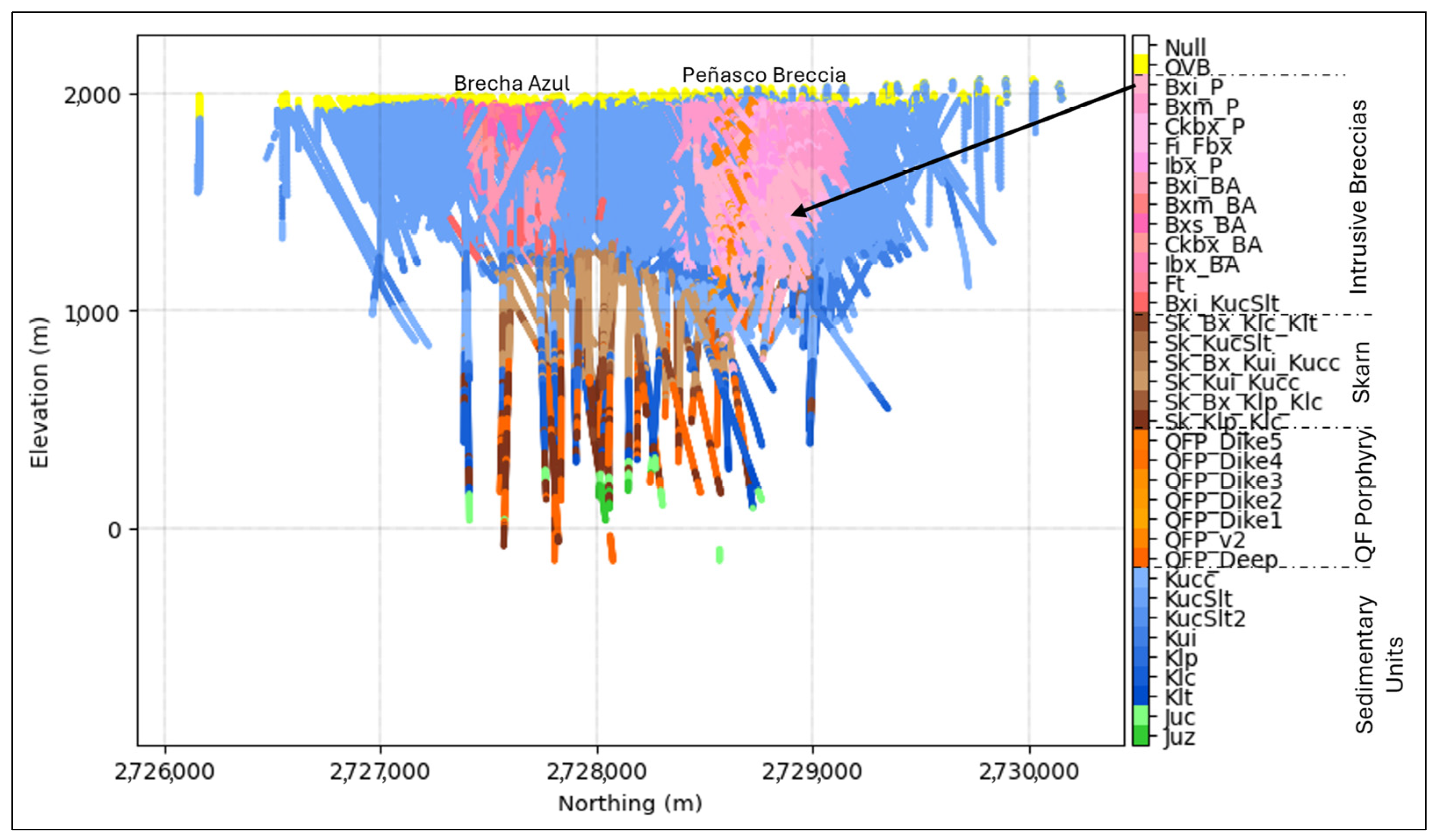
Building on the proposed methodology, this case study applies the enhanced multivariate simulation workflow to the intrusive breccia (Bxi_P) domain characterized by strong QSP alteration. This high-grade domain within the Peñasco breccia complex represents the core of the deposit. Figure 2 displays a north–south lithology section highlighting multiple breccia domains in shades of pink, which also includes the Bxi_P domain.

The goal of this case study is to demonstrate the implementation of the proposed workflow and its impact on the results, with a focus on data reproduction.

3.1. Dataset Overview

The dataset consisted of 7946 samples (4 m composites) with assays for Au, Ag, Pb, and Zn, which were sampled equally. Univariate capping was applied to the composites as follows: Au at 35 ppm, Ag at 640 ppm, Pb at 9%, and Zn at 11%. The samples were collected using two drilling methods: DDH preferentially, with fewer RC drill holes restricted to the northwest portion of the domain. In total, the dataset consists of 297 DDH holes representing 7685 samples and nine RC holes representing 261 samples. The drill hole pattern consisted of a combination of vertical and inclined drill holes, covering an area of approximately 800 m by 800 m that extended to a maximum vertical depth of approximately 1200 m from the surface. The drilling pattern was irregular, with an average spacing of approximately 30 m. The eastern portion of the domain exhibits a tighter drill spacing, which follows a circular pattern close to the breccia domain boundary.

Analyzing the main characteristics of this dataset provided a robust foundation for the subsequent bias correction and multivariate outlier treatment steps, which are critical for improving the simulation results.

3.2. Univariate and Multivariate Statistics

The grade distributions of Au, Ag, Pb, and Zn within the selected domain exhibited significant variability, particularly in relation to elevation. The highest concentrations of these metals were generally observed between elevations of 1400 m and 1650 m. Silver exhibits elevated values at higher elevations, reflecting a cupola-shaped geometry, as shown in Figure 3. All four variables exhibit a positively skewed distribution. Despiking is necessary because of 238 repeated values in the Au dataset at the detection limit of 0.025 ppm [36], a common issue in geochemical datasets that can distort statistical analyses [37]. A multivariate despiking approach was applied using the rmsp.DespikeMVSpatial method [37] to address these spikes while preserving variable relationships and spatial continuity.

High-grade areas often contain more drill holes, whereas low-grade regions tend to have fewer drill holes. Declustering helps correct this imbalance by assigning weights to the data, allowing both densely and sparsely sampled areas to contribute to the analysis properly. An inverse distance declustering approach is used to obtain representative statistics for each variable.

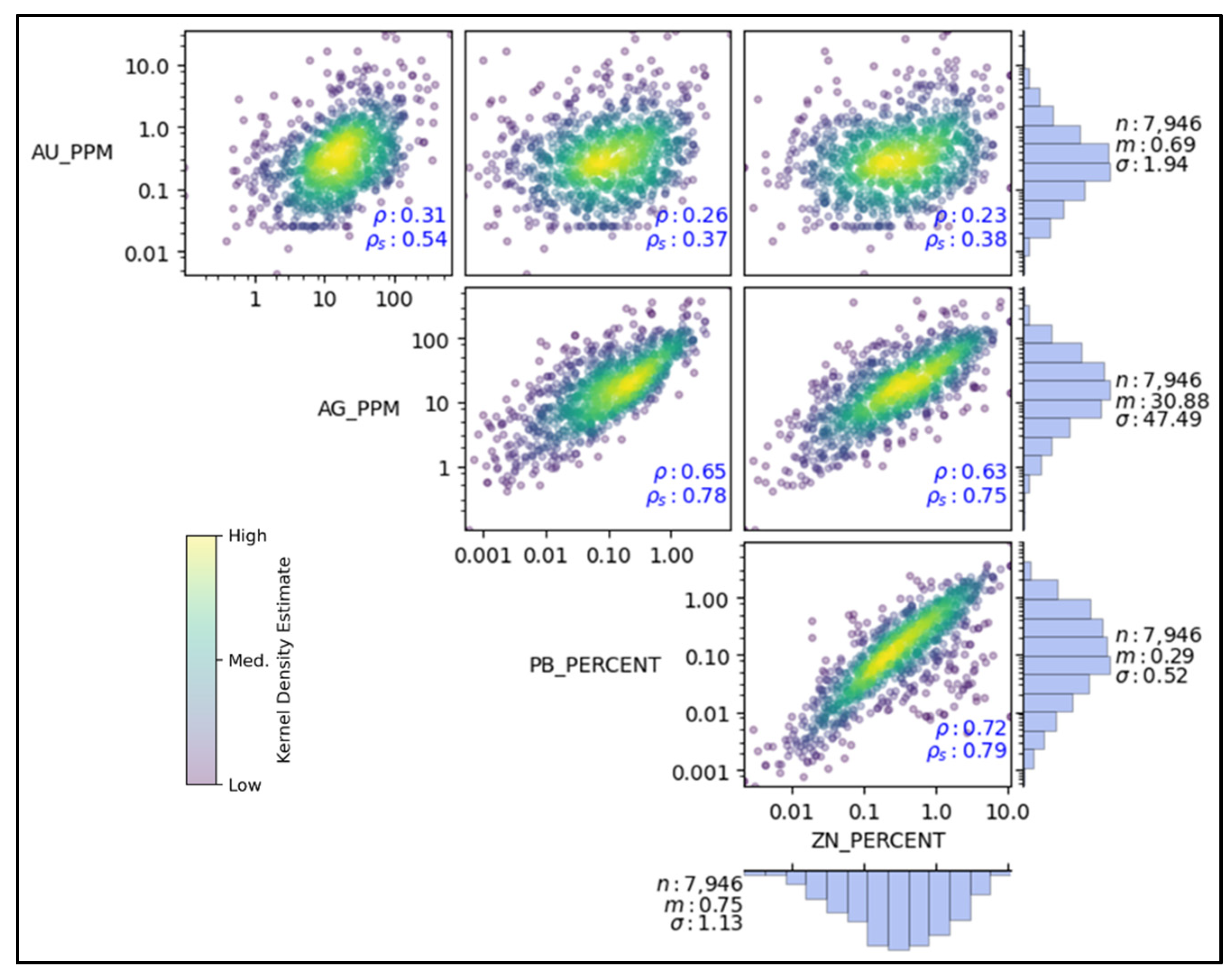
Multivariate analysis showed complex, non-linear relationships. The correlations between Au and the other variables were low, whereas Ag showed a moderate correlation with Pb and Zn. The strongest correlation was observed between Pb and Zn. Both Pearson and Spearman coefficients were used to characterize these relationships. Scatter plots of the declustered values for Au, Ag, Pb, and Zn are shown in Figure 4. The declustered histograms (on a logarithmic scale) were displayed along the margins of each variable axis to provide context with scatter plot information. The mean values for the variables were as follows: 0.69 ppm for Au, 30.88 ppm for Ag, 0.29% for Pb, and 0.75% for Zn.

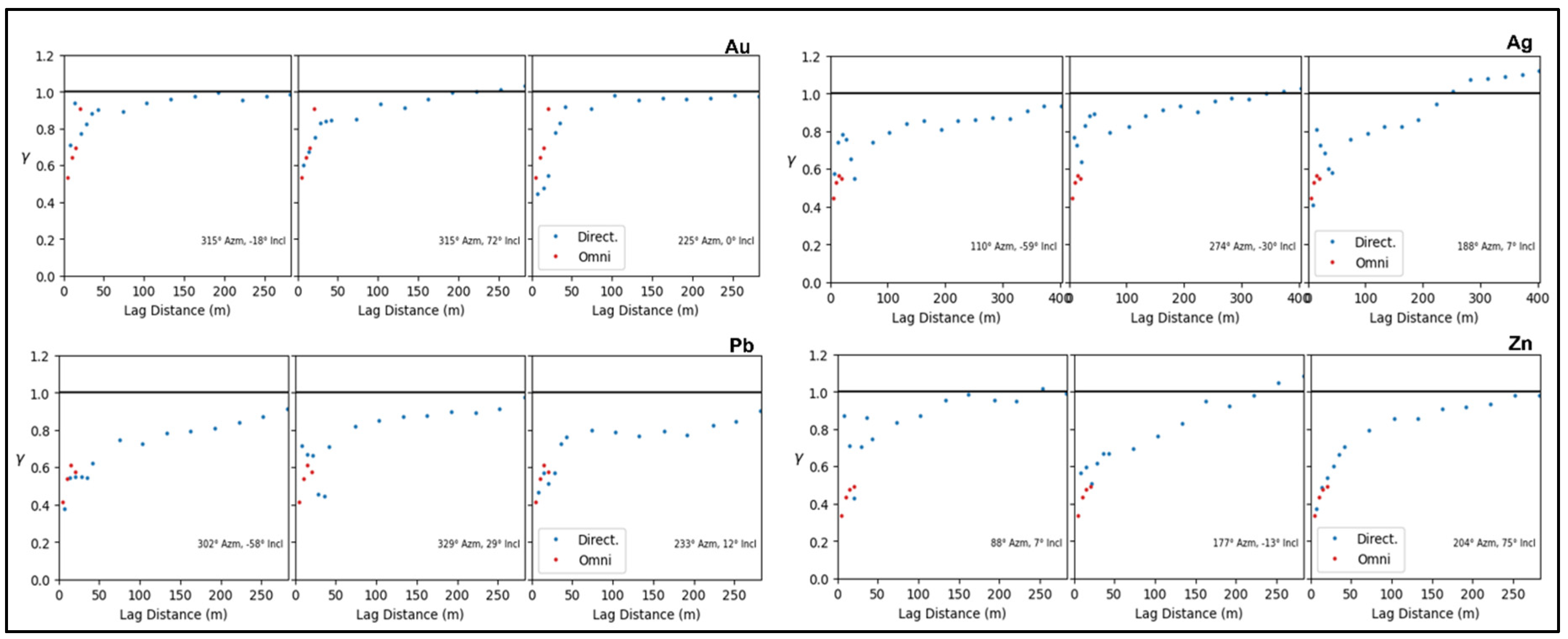
Variogram analysis indicated weak anisotropy with subtle preferential continuity directions. The variogram ranges for Au and Ag were 200–250 m, whereas Pb and Zn exhibited a much larger range of 250–350 m. Figure 5 shows the experimental variograms in the three principal directions for Au, Ag, Pb, and Zn.

3.3. Bias Correction and Outlier Treatment

The pairing analysis for the breccia domain showed a significant bias between the RC and DDH datasets. For RC drill holes, Au means were 227% higher in comparison to DDH means. Ag, Pb, and Zn showed bias, but were less extreme. Limited RC data resulted in only a small number of pairs, with a maximum of 12 in this domain. To correct this bias, the mean and standard deviation differences from the pairing analysis were used to infer adjusted DDH statistics. RC data were standardized to a mean of zero and a standard deviation of one, then transformed back using the inferred DDH statistics. This approach was validated in another domain with more extensive RC-DDH drill hole pairs, thereby providing confidence in its application. The correction was applied to all the RC samples.

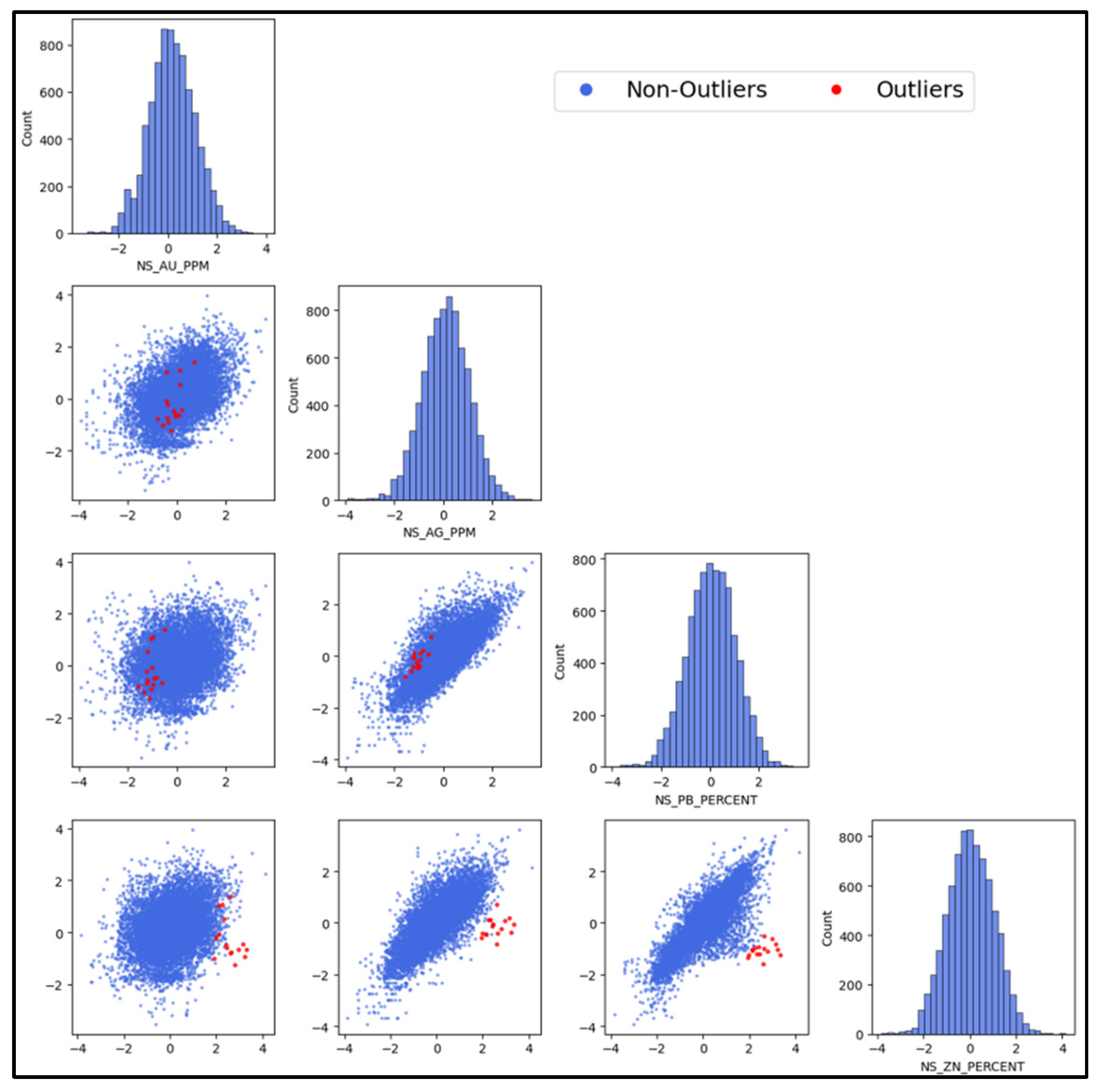
Following bias correction, the next step in the workflow addresses multivariate outliers to ensure that extreme values do not distort the variograms, trends, or decorrelation results. Multivariate outlier detection was performed to identify any remaining extreme values that could affect the simulation outcomes. Because the variables were reported in different units (ppm to percent), the data were first transformed into a normal score unit to ensure that no single variable dominated the Mahalanobis distance calculation. The Robust Mahalanobis distance (MCD) was calculated, and a capping threshold was selected using a combination of tools, including scatter plots, variogram clouds, and a QQ plot comparing the Mahalanobis distance with theoretical chi-squared quantiles. A high Mahalanobis distance indicates a higher probability of a potential multivariate outlier. Based on these evaluations, multivariate capping was applied at the 99.80th percentile, corresponding to a Mahalanobis distance of 76.35, as shown in Figure 6. Applying multivariate capping at the 99.80th percentile managed the presence of extreme outliers and improved the model. This threshold was evaluated against alternative approaches (standardized data only, classical Mahalanobis distance, and robust Mahalanobis distance). Cross-validation using RMSE, R², and Spearman correlation confirmed that the 99.8% cutoff provided the best result. This approach is not overly aggressive and has resulted in minimal metal loss.

3.4. Data Division for Modeling and Validation

A regular modeling grid (5 m × 5 m × 5 m) was used within the selected domain, resulting in approximately 0.511 million blocks. In order to evaluate the workflows, the data were randomly divided into two subsets: approximately 95% of the samples (7569 from 292 drill holes) were used as modeling data, whereas the remaining 5% (377 from 14 drill holes) were reserved as test data (RC data were not included). Figure 7a presents a plan view of the drill hole traces for both test and modeling data, while Figure 7b provides a 3D view of the same dataset, with traces colored by Au values.

The goal is to compare two workflows: (1) the current workflow, which applies trend modeling followed by a single PPMT, and (2) the proposed workflow, which applies PPMT before trend modeling and then after trend removal.

The modeling data were used for simulation and to evaluate histograms, variograms, correlation coefficients, and multivariate reproduction features. The test data were used for cross-validation of the model performance using the root mean squared error (RMSE) and Spearman correlation.

3.5. Workflow Implementation After Multivariate Outlier Treatment

With bias correction completed and multivariate outliers managed, the workflow proceeded to trend modeling and decorrelation, both of which are critical in preparing the data for accurate Gaussian simulation.

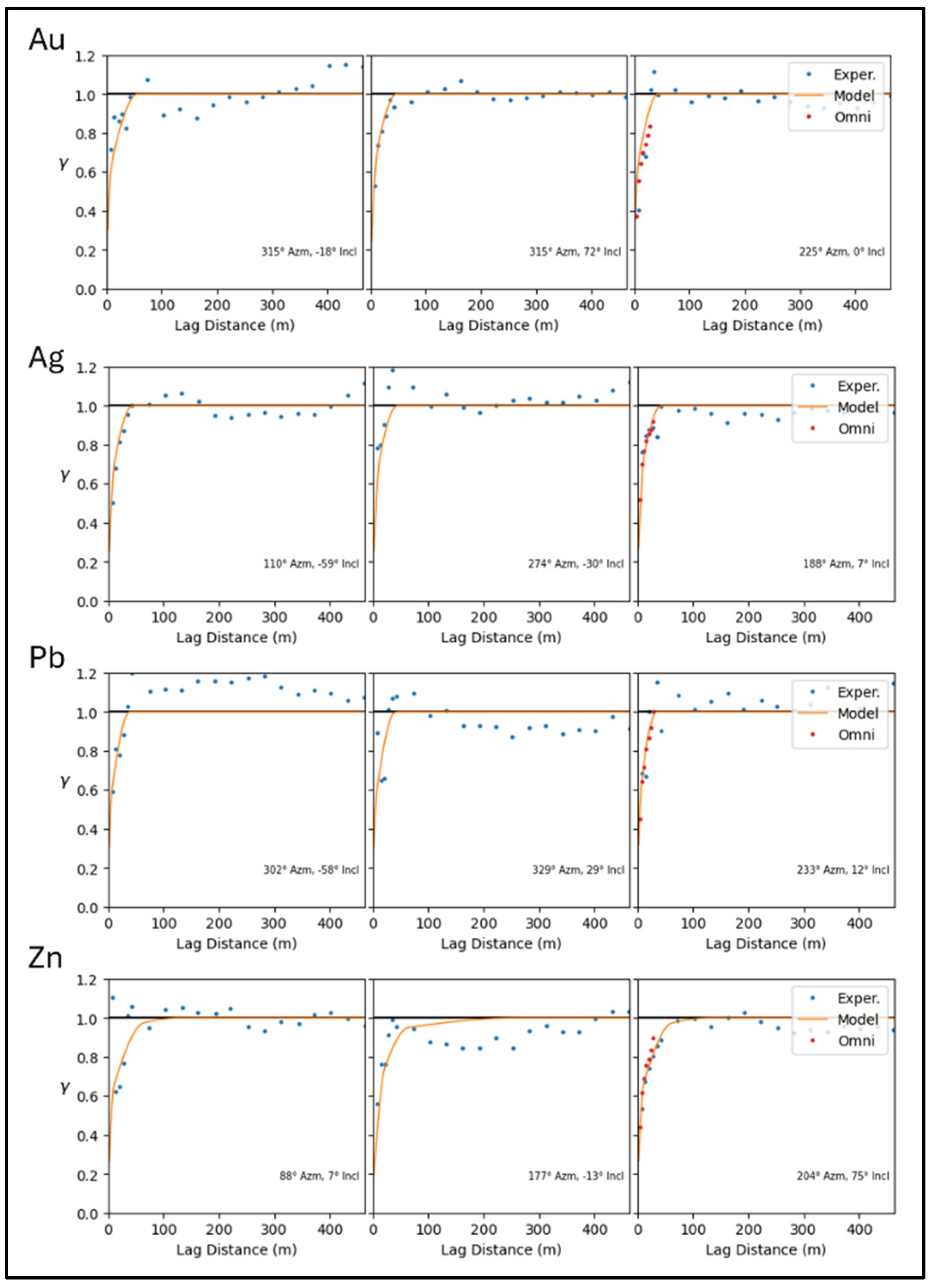
Following multivariate outlier treatment, trend modeling was performed in normal score (NS) units applying an MWA approach with up to 600 samples and a smoothing factor of 1.8 to minimize residual correlation. The resulting trend models captured spatial patterns across the domain, with moderate-to-strong correlations (ρ and ρs ranging from 0.60 to 0.75) between the sample data and the modeled trends, indicating non-stationarity. The trend dependency with the data values is then removed using the GMM, which includes declustering weights and several kernels set to 3. Then, SCT is performed using the conditional distributions obtained from the GMM. After trend removal, the residuals showed almost no correlation with the trends, with values near zero. Experimental variograms were modeled for the residuals of Au, Ag, Pb, and Zn. Nested spherical models were used with ranges of 12 m and 60 m for Au, Ag, Pb, and Zn, ranging from 14 to 125 m in the main direction, as shown in Figure 8. This figure displays the variogram models in the three main directions for each variable. These variogram models were used for Gaussian simulations. The variograms indicate isotropic to weak anisotropic characteristics within this domain. In the standard workflow, PPMT was applied to decorrelate the residuals prior to simulations.

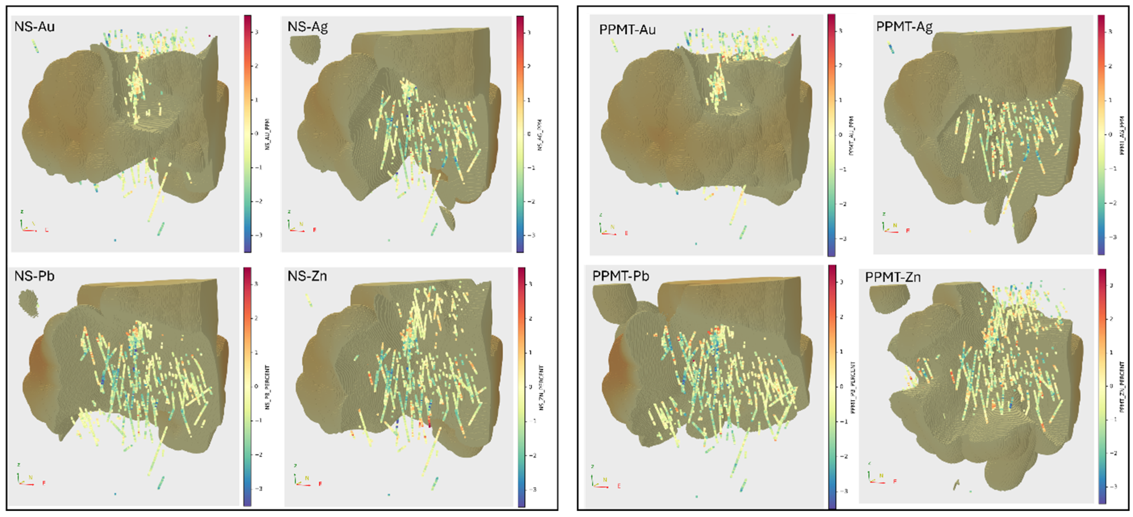
In the proposed workflow, PPMT-1 was first applied (targeting normality at the 50th percentile, with 150 iterations), and trend modeling was then conducted on the PPMT-1 variables. The resulting trend models for Au, Ag, and Pb were generally similar across both workflows. The Zn model in this workflow captured the high-grade zone located near the bottom center of the domain more effectively (Figure 9).

After detrending, the second PPMT2 transformation (targeting normality at the 50th percentile, with 100 iterations) produced fully independent variables with near-zero correlations and standard normal distributions.

Importantly, simulation was independently performed for each variable. After the Gaussian simulations were completed on the PPMT-2 variables, the results were sequentially back-transformed to the original units.

4. Results

This section compares the proposed workflow with the standard approach, focusing on data reproduction, variogram and histogram reproduction, preservation of multivariate structure, and cross-validation accuracy.

The proposed workflow, which addresses data bias, multivariate outliers, trend modeling, and decorrelation, is compared with the standard workflow to assess performance, particularly with a focus on simulation accuracy and data reproduction.

The evaluations included histogram reproduction of the 100 realizations against the sample data, as well as comparisons of the variogram and cross-variogram between the experimental variogram of the sample data and the variogram models of the 100 realizations. Lastly, scatter plots were generated to assess the reproduction of bivariate features using one realization as an example. The correlation matrices of the sample data are compared with the average correlations of 100 realizations. Cross-validation results are presented to compare the test dataset against the simulation outcomes. The root mean squared error (RMSE) and Spearman’s correlation are evaluated to measure the model’s performance.

The results from both the standard workflow and the proposed workflow for Au, Ag, Pb, and Zn are presented side by side to compare visually the differences in performance.

4.1. Data Reproduction

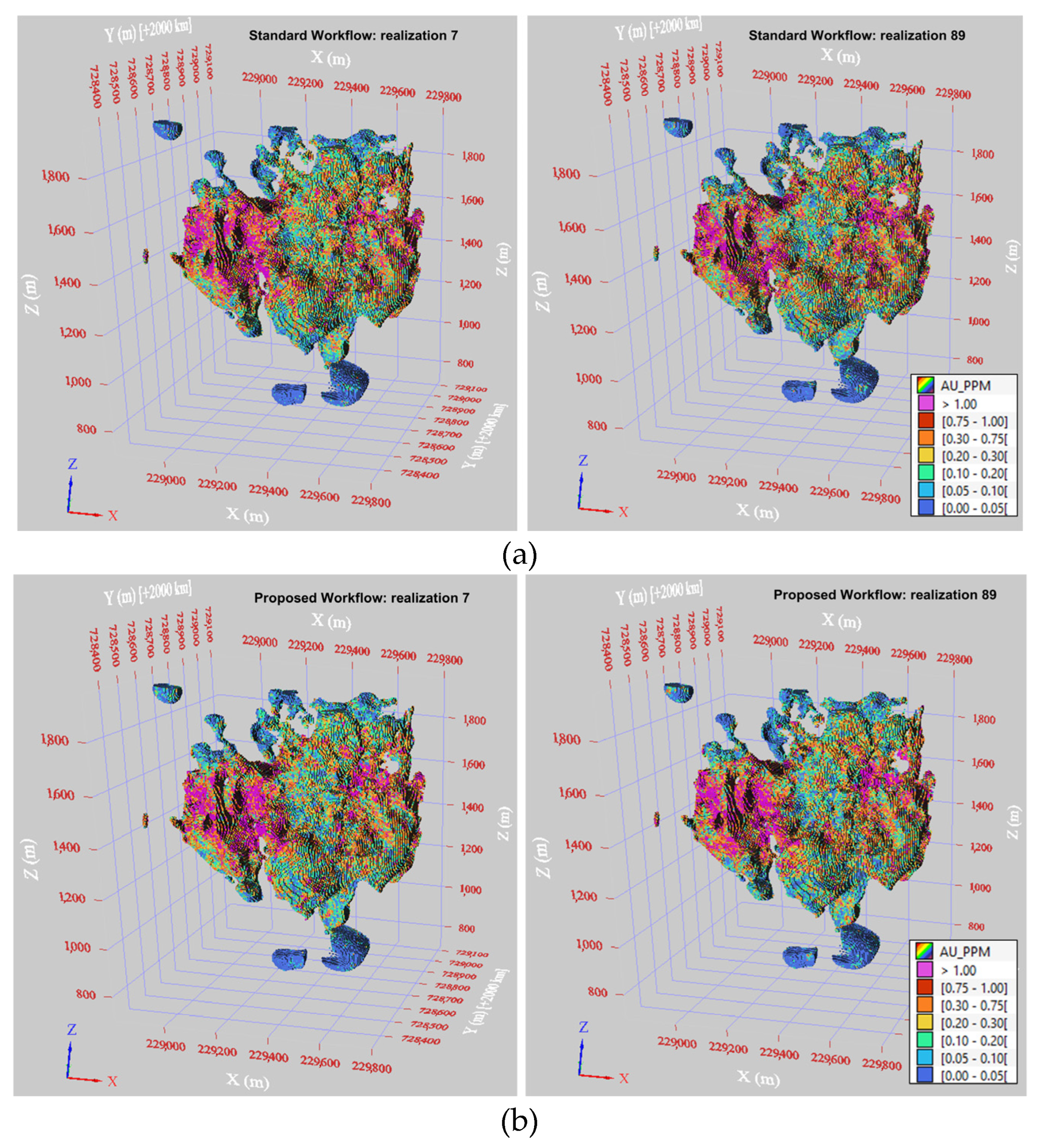
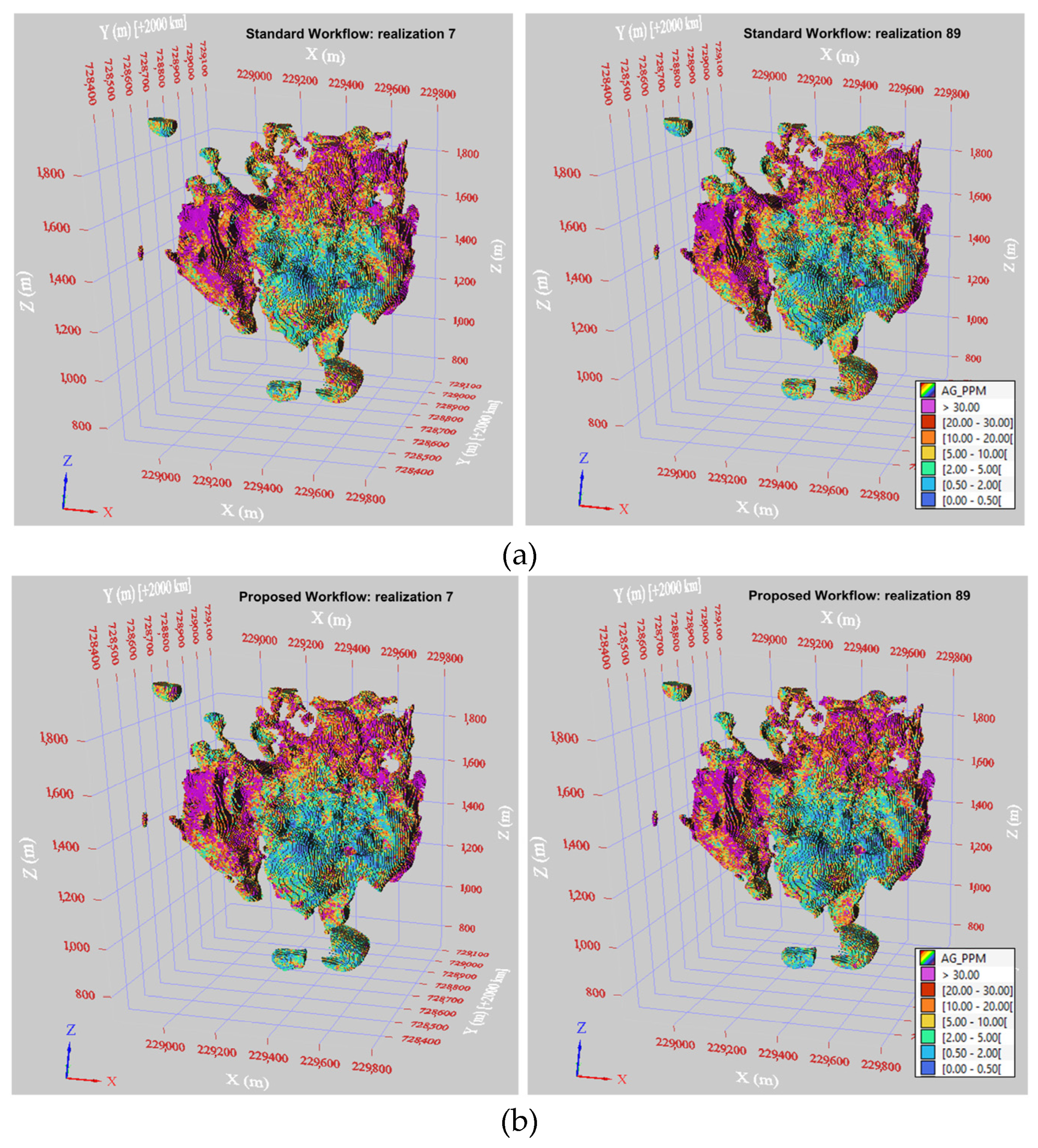
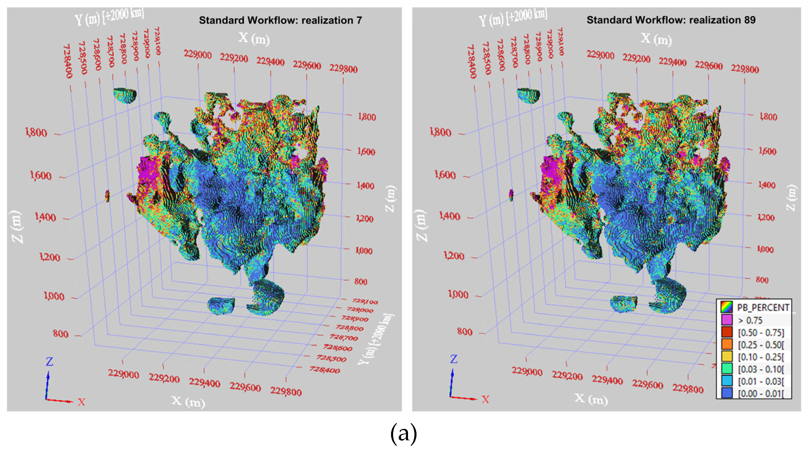
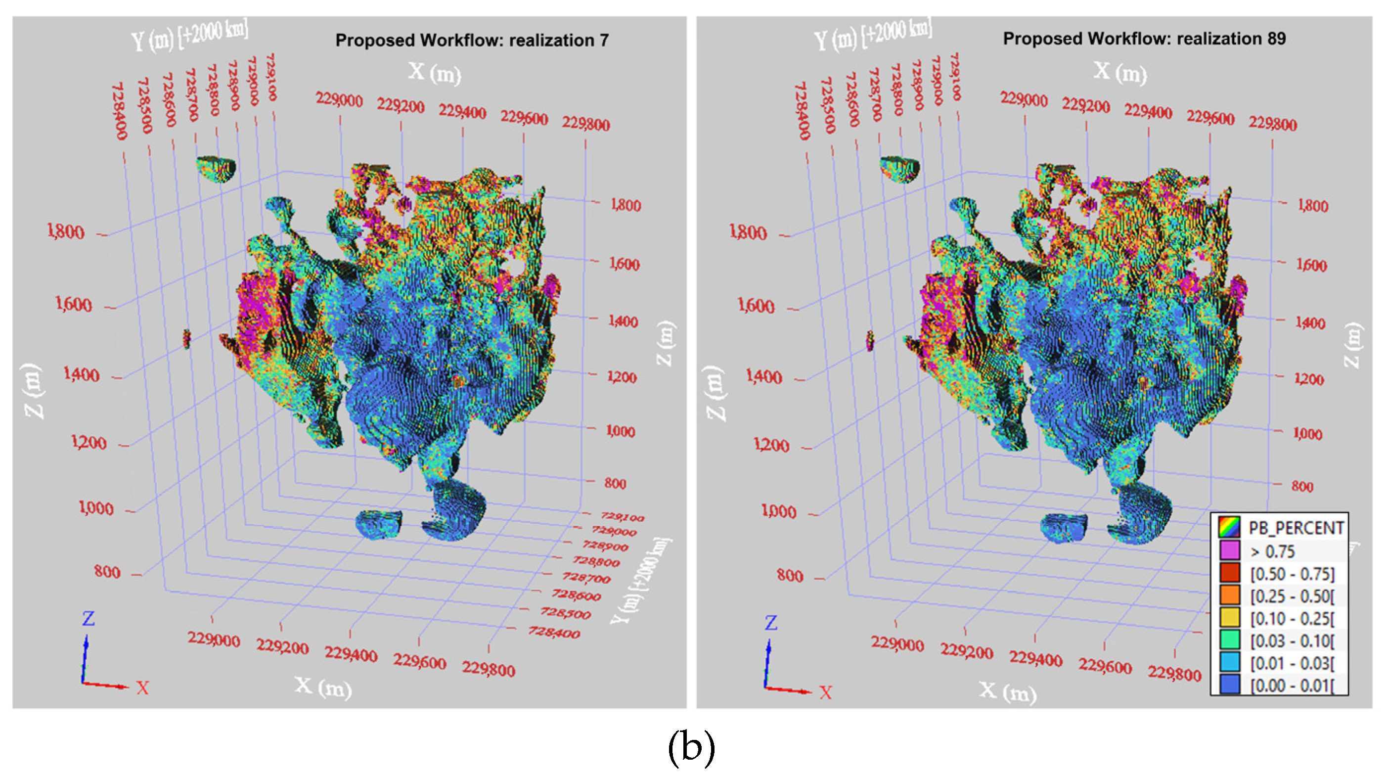
Visual data reproduction is presented in Figure 10, Figure 11, Figure 12 and Figure 13, which show 3D views of the simulation results for Au, Ag, Pb, and Zn, across two realizations (7 and 89). In each figure, (a) shows the standard workflow results, and (b) shows the outcomes of the proposed workflow.

The two realizations effectively reproduce the high and low-grade areas, as observed in the drill hole data (Figure 3), without any artifacts. The high-grade cupola feature shown in magenta is more evident in the Ag realizations.

The results from the proposed workflow show slight differences compared with the standard workflow. Notably, for Ag, the lower-grade area located at the bottom of the domain is better reproduced using the proposed workflow.

For Zn, the proposed workflow results indicate that high-grade areas are slightly more limited than those seen in the standard workflow results.

4.2. Histogram and Global Statistics Reproduction

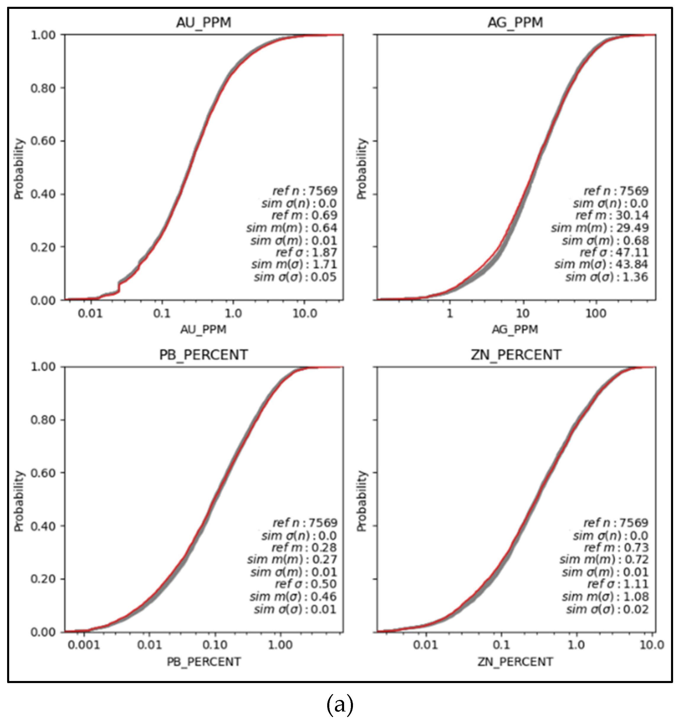
Figure 14a shows the histogram reproduction of Au, Ag, Pb, and Zn in the original units for the standard workflow. The red line represents the histogram for the modeling data, whereas the gray lines represent the histograms from 100 realizations. The average value of the simulations was lower than the modeling data, exhibiting 7% lower values for Au, 2% lower values for Ag, 3.5% lower values for Pb, and 0.14% lower values for Zn. Overall, the global distribution of Au, Pb, and Zn shows strong reproduction. However, the reproduction of Ag did not yield satisfactory results between 1 ppm and 10 ppm, as indicated by the noticeable gap between the realizations and the sample data shown in red. Figure 14b shows the histogram reproduction for Au, Ag, Pb, and Zn used in the proposed workflow. The average grades are very similar to those presented in Figure 14a. Regarding Ag, the previous discrepancy between 1 and 10 ppm was addressed, and the issue of reproduction was resolved. The global distributions of Au, Pb, and Zn exhibited good reproduction.

4.3. Variogram and Cross-Variogram Reproduction

The reproduction of the spatial variability between the sampled data and the generated realizations is illustrated through variograms and cross-variograms. An omnidirectional is used to display the variograms and cross-variograms for Au, Ag, Pb, and Zn in Figure 15. The red dots represent the experimental variograms of the modeling data, while the gray lines show the variogram models of the 100 realizations. Results show good reproduction of the variograms and cross-variograms.

4.4. Correlation Matrices and Multivariate Reproduction

The multivariate reproduction for Au, Ag, Pb, and Zn is illustrated using scatter plots to evaluate how well complex bivariate features are reproduced in the realizations. Figure 16a shows scatter plots of the modeling data (declustered) on the left and realization 1, using the standard workflow on the right. The scatter plots are color-coded using kernel density estimation (KDE) to help visualize data density and underlying patterns. While the relationships are reasonably reproduced, Ag/Pb, Ag/Zn, and Pb/Zn remain less satisfactory. This is also evident for the Pb/Zn relationships, where the sample data show an elongated ellipse, while realization 1 appears wider. Figure 16b illustrates the modeling data on the left and Realization 1 using the proposed workflow on the right. The reproduction of bivariate relationships improves notably for Ag/Pb, Ag/Zn, and Pb/Zn. Notably, the Pb/Zn relationship now captures the elongated features seen in the sample data.

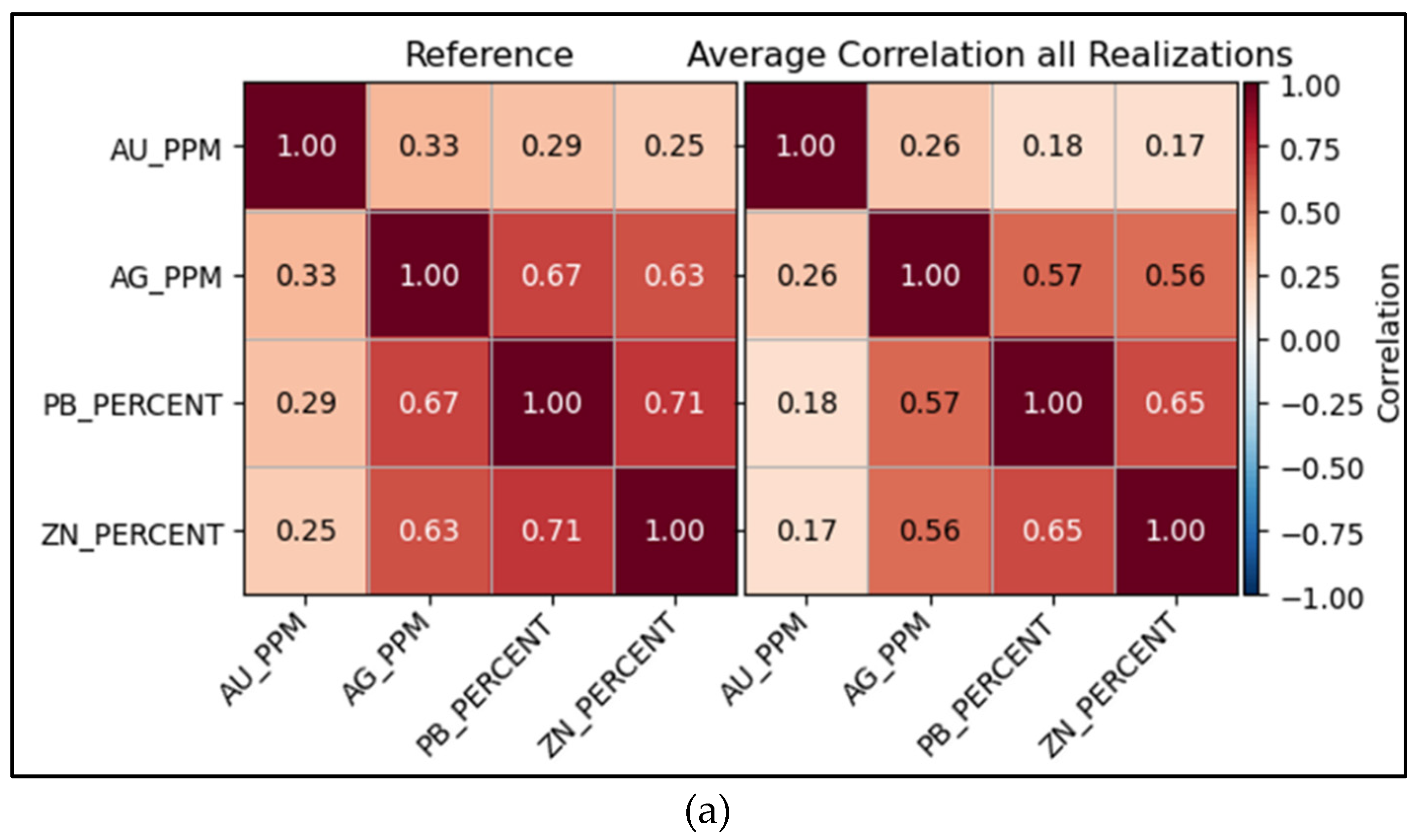
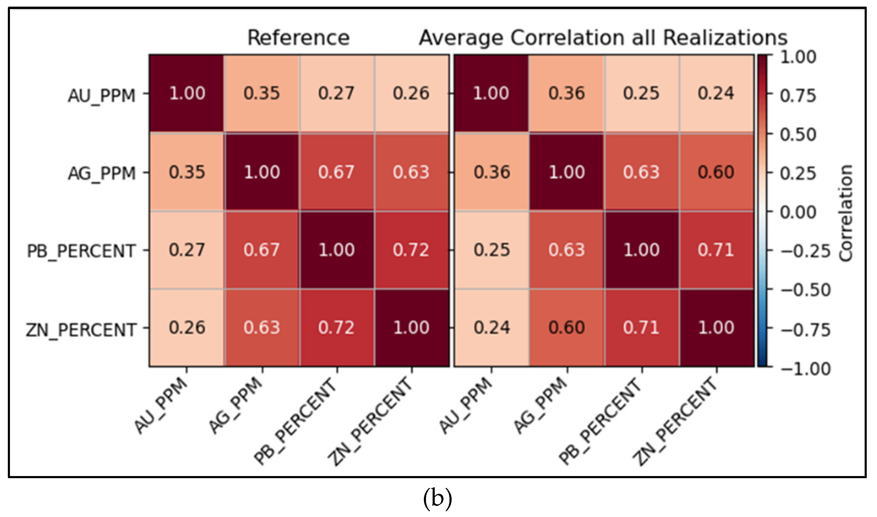
The correlation matrices further compare the modeling data with an average of 100 realizations. Figure 17a shows Pearson correlations for the standard workflow, with the modeling data displayed on the left and the realizations on the right. The comparisons show the correlations for Au/Ag, Au/Pb, and Au/Zn from the realizations are as much as 38% lower than those observed in the sample data. In comparison, Figure 17b shows the proposed workflow, with the Pearson correlation of the modeling data on the left and the realizations on the right. In this case, the correlations are only 7.7% lower than those obtained from the sample data. This represents a significant improvement, particularly for Au/Ag, Au/Pb, and Au/Zn correlations.

4.5. Cross-Validation Results

Cross-validation compares the true values (377 samples) with the E-type (average of 100 realizations) using the following metrics:

(i) Mean of realizations vs. true mean,

(ii) Mean standard deviation of realizations vs. true standard deviation (noting expected differences due to smoothing),

(iii) Spearman correlation (ρs), where higher values indicate better correlation, and

(iv) RMSE, where lower values indicate a better fit.

Table 1. (a). Cross-validation results for Au and Ag. (b). Cross-validation results for Pb and Zn.

Cross-Validation	(a)										(b)
	Au ppm					Ag ppm					Pb%					Zn%
Simulated values against Test data	Etype (μ)	True (μ)	Spearman Correlation	RMSE	R2	Etype (μ)	True (μ)	Spearman Correlation	RMSE	R2	Etype (μ)	True (μ)	Spearman Correlation	RMSE	R2	Etype (μ)	True (μ)	Spearman Correlation	RMSE	R2
Standard Workflow	0.73	0.69	0.55	1.52	0.09	33.49	43.01	0.71	40.76	0.24	0.31	0.48	0.71	0.69	0.18	0.88	1.26	0.57	1.42	0.14
Proposed Workflow	0.72	0.69	0.58	1.43	0.11	33.96	43.01	0.70	40.58	0.25	0.31	0.47	0.73	0.62	0.21	0.90	1.25	0.58	1.39	0.16
Standard Workflow vs. Proposed Workflow			5.45%	−5.92%	22.22%			−1.41%	−0.44%	4.17%			2.82%	−10.14%	16.67%			1.75%	−2.11%	14.29%

a,b summarize the cross-validation results comparing the standard and proposed workflows. For the standard workflow, the mean of the realizations (Etype) is lower than the true values for Ag, Pb, and Zn, and slightly higher for Au. The Spearman correlations for the proposed workflow are slightly higher for Au, Pb, and Zn. Also, the RMSE results for the proposed workflow show consistent improvements across all variables. In comparison to the standard workflow, Pb and Au yielded the best improvements, ranging from 6% to 10%. In the case of the R² for the proposed workflow, the improvements range from 4% to 22% compared to the standard workflow. Overall, these results indicate a better model performance in the proposed workflow.

5. Discussion and Conclusions

This case study focuses on a new workflow for a high-grade polymetallic domain with strong non-stationarity to improve models with better data statistics reproduction. This was accomplished by addressing: data bias, multivariate outliers, trend modeling, and the application of PPMT before and after trend modeling.

The results demonstrated clear improvements when compared with the standard approach. Data standardization after bias analysis mitigated the biases introduced by RC drill holes. This was followed by applying the Mahalanobis distance to detect multivariate outliers and capping at an appropriate percentile, which further improved the outcomes. Finally, applying PPMT twice addressed strong non-stationarity more effectively than using a single transformation (NS units) before modeling the trends. Notably, the Zn trend model exhibited a slightly different pattern from the proposed workflow.

In conclusion, the proposed framework consistently improved the reproduction of histograms, variograms, correlation coefficients, and bivariate features, while also reducing RMSE and improving R² in cross-validation.

Some limitations of the proposed workflow included managing multivariate outliers. This requires experienced judgment to select appropriate capping thresholds. However, cross-validation, along with other statistical tools (such as QQ plots and scatter plots), can assist in making a final decision. Importantly, future research should investigate the trade-off between preserving correlation and the risk of over-smoothing high-grade values. Another limitation involves trend modeling optimization, where the trend residual correlation plot was ineffective in determining the optimal number of composites to use. This process is challenging because it requires multiple tests that may introduce some subjectivity into this step.

After applying the PPMT twice, still weak remnant correlations remained between the variables, as observed in the cross variograms. Future research should investigate whether full decorrelation is possible and how this could impact simulation results.

Lastly, while this study was conducted on a complex epithermal, polymetallic domain, further validation of this proposed workflow is recommended across multiple geologic settings.

References

- Rossi, M.E.; Deutsch, C.V. Mineral Resource Estimation; Springer Science & Business Media: Berlin, Germany, 2013. [Google Scholar]
- Dias, P.M.; Deutsch, C.V. The Decision of Stationarity. Geostatistics Lessons. 2022. Available online: https://geostatisticslessons.com/pdfs/stationarity.pdf (accessed on 15 August 2024).
- Qu, J.A. Practical Framework to Characterize non-Stationary Regionalized Variables. Ph.D. Thesis, University of Alberta, Edmonton, AB, Canada, 2018. [Google Scholar]
- Manchuk, J.; Deutsch, C.V. A Short Note on Trend Modeling Using Moving Windows. Centre for Computational Geostatistics Annual Report: Edmonton, AB, Canada, 2011. [Google Scholar]
- Isaaks, E.H.; Srivastava, R.M. Applied Geostatistics; Oxford University Press: New York, NY, USA, 1989. [Google Scholar]
- Harding, B.; Deutsch, C.V. Trend Modeling and Modeling with a Trend. Geostatistics Lessons. 2021. Available online: https://geostatisticslessons.com/pdfs/trendmodeling.pdf (accessed on 15 January 2025).
- Qu, J.; Deutsch, C.V. Geostatistical simulation with a trend using Gaussian mixture models. Nat. Resour. Res. 2018, 27, 347–363. [Google Scholar] [CrossRef]
- Rosenblatt, M. Remarks on a multivariate transformation. Ann. Math. Stat. 1952, 23, 470–472. [Google Scholar] [CrossRef]
- Leuangthong, O.; Deutsch, C.V. Transformation of residuals to avoid artifacts in geostatistical modelling with a trend. Math. Geol. 2004, 36, 287–305. [Google Scholar] [CrossRef]
- Journel, A.G.; Huijbregts, C.J. Mining Geostatistics; Academic Press: London, UK, 1978. [Google Scholar]
- Goovaerts, P. Geostatistics for Natural Resources Evaluation; Oxford University Press: New York, NY, USA, 1997. [Google Scholar]
- Wackernagel, H. Multivariate Geostatistics: An Introduction with Applications; Springer Science & Business Media: Berlin, Germany, 2003. [Google Scholar]
- Chiles, J.P.; Delfiner, P. Geostatistics: Modeling Spatial Uncertainty; John Wiley & Sons: Hoboken, NJ, USA, 2012. [Google Scholar]
- Pearson, K. LIII. On lines and planes of closest fit to systems of points in space. Lond. Edinb. Dublin Philos. Mag. J. Sci. 1901, 2, 559–572. [Google Scholar] [CrossRef]
- Hotelling, H. Analysis of a complex of statistical variables into principal components. J. Educ. Psychol. 1933, 24, 498–520. [Google Scholar] [CrossRef]
- Hwang, J.N.; Lay, S.R.; Lippman, A. Nonparametric multivariate density estimation: A comparative study. IEEE Trans. Signal Process. 1994, 42, 2795–2810. [Google Scholar] [CrossRef]
- Desbarats, A.J.; Dimitrakopoulos, R. Geostatistical simulation of regionalized pore-size distributions using min/max autocorrelation factors. Math. Geol. 2000, 32, 919–942. [Google Scholar] [CrossRef]
- Leuangthong, O.; Deutsch, C.V. Stepwise conditional transformation for simulation of multiple variables. Math. Geol. 2003, 35, 155–173. [Google Scholar] [CrossRef]
- Fukunaga, K. Introduction to Statistical Pattern Recognition; Elsevier: Amsterdam, The Netherlands, 2013. [Google Scholar]
- Barnett, R.M. Managing Complex Multivariate Relations in the Presence of Incomplete Spatial Data. Ph.D. Thesis, University of Alberta, Edmonton, AB, Canada, 2015. [Google Scholar]
- Van den Boogaart, K.G.; Mueller, U.; Tolosana-Delgado, R. An affine equivariant multivariate normal score transform for compositional data. Math. Geosci. 2017, 49, 231–251. [Google Scholar] [CrossRef]
- Tolosana-Delgado, R.; Mueller, U. Geostatistics for Compositional Data with R; Springer Cham: Cham, Switzerland, 2021. [Google Scholar]
- Avalos, S.; Ortiz, J.M. Spatial multivariate morphing transformation. Math. Geosci. 2023, 55, 735–771. [Google Scholar] [CrossRef]
- Barnett, R.M.; Manchuk, J.; Deutsch, C.V. The projection-pursuit multivariate transform for improved continuous variable modeling. SPE Journal. 2016, 21, 2010–2026. [Google Scholar] [CrossRef]
- Leuangthong, O.; McLennan, J.A.; Deutsch, C.V. Minimum acceptance criteria for geostatistical realizations. Nat. Resour. Res. 2004, 13, 131–141. [Google Scholar] [CrossRef]
- Deutsch, C.V. Checking Continuous Variable Realizations-Mining. Geostatistics Lessons. 2017. Available online: https://geostatisticslessons.com/pdfs/checkingmin.pdf (accessed on 17 November 2024).
- Teal, R.M. An Innovative Framework for Multivariate Simulation Within Non-Stationary Domains. Ph.D. Thesis, New Mexico Institute of Mining and Technology, Socorro, NM, USA, 2025. [Google Scholar]
- Resource Modeling Solutions Ltd. Documentation. Available online: https://portal.resourcemodelingsolutions.com/doc/overview.html (accessed on 15 December 2024).
- Mahalanobis, P.C. On the generalized distance in statistics. Proc. Natl. Inst. Sci. India 1936, 12, 49–55. [Google Scholar]
- Leys, C.; Klein, O.; Dominicy, Y.; Ley, C. Detecting multivariate outliers: Use a robust variant of the Mahalanobis distance. J. Exp. Soc. Psychol. 2018, 74, 150–156. [Google Scholar] [CrossRef]
- Friedman, J.H. Exploratory projection pursuit. J. Am. Stat. Assoc. 1987, 82, 249–266. [Google Scholar] [CrossRef]
- Barnett, R.M. Sphereing and Min/Max Autocorrelation Factors. Geostatistics Lessons; Deutsch, J.L., Ed. 2017. Available online: https://geostatisticslessons.com/pdfs/sphereingmaf.pdf (accessed on 15 August 2023).
- Matheron, G. The intrinsic random functions and their applications. Adv. Appl. Probab. 1973, 5, 439–468. [Google Scholar] [CrossRef]
- Journel, A.G. Geostatistics for conditional simulation of ore bodies. Econ. Geol. 1974, 69, 673–687. [Google Scholar] [CrossRef]
- Dromundo, O.; Robles, S.; Bissig, T.; Flores, C.; del Carmen Alfaro, M.; Cardona, L. The Peñasquito Gold-(Silver-Lead-Zinc) Deposit; Society of Economic Geologists: Zacatecas, Mexico, 2020. [Google Scholar]
- Teal, R.M. Data analysis for multivariate simulations in complex, non-stationary domains. Prof. Geologist. 2025, 62, 6–16. [Google Scholar]
- Pyrcz, M.J.; Deutsch, C.V.; Deutsch, J.L. Transforming Data to a Gaussian Distribution. Geostatistics Lessons. 2018. Available online: https://geostatisticslessons.com/pdfs/normalscore.pdf (accessed on 17 June 2023).