Article

Geometallurgical Cluster Creation in a Niobium Deposit Using Dual-Space Clustering and Hierarchical Indicator Kriging with Trends

by
João Felipe C. L. Costa
1,
Fernanda G. F. Niquini
1,*,
Claudio L. Schneider
2,
Rodrigo M. Alcântara
3,
Luciano N. Capponi
3 and
Rafael S. Rodrigues
3
1
Departamento de Engenharia de Minas, Universidade Federal do Rio Grande do Sul, Porto Alegre 91501-970, RS, Brazil
2
Centro de Tecnologia Mineral (CETEM), Rio de Janeiro 21941-908, RJ, Brazil
3
Companhia Brasileira de Metalurgia e Mineração (CBMM), Araxa 38183-903, MG, Brazil
*
Author to whom correspondence should be addressed.
Minerals 2025, 15(7), 755; https://doi.org/10.3390/min15070755
Submission received: 8 May 2025 / Revised: 17 June 2025 / Accepted: 2 July 2025 / Published: 19 July 2025
(This article belongs to the Special Issue Geostatistical Methods and Practices for Specific Ore Deposits)

Abstract

Alkaline carbonatite complexes are formed by magmatic, hydrothermal, and weathering geological events, which modify the minerals present in the rocks, resulting in ores with varied metallurgical behavior. To better spatially distinguish ores with distinct plant responses, creating a 3D geometallurgical block model was necessary. To establish the clusters, four different algorithms were tested: K-Means, Hierarchical Agglomerative Clustering, dual-space clustering (DSC), and clustering by autocorrelation statistics. The chosen method was DSC, which can consider the multivariate and spatial aspects of data simultaneously. To better understand each cluster’s mineralogy, an XRD analysis was conducted, shedding light on why each cluster performs differently in the plant: cluster 0 contains high magnetite content, explaining its strong magnetic yield; cluster 3 has low pyrochlore, resulting in reduced flotation yield; cluster 2 shows high pyrochlore and low gangue minerals, leading to the best overall performance; cluster 1 contains significant quartz and monazite, indicating relevance for rare earth elements. A hierarchical indicator kriging workflow incorporating a stochastic partial differential equation (SPDE) trend model was applied to spatially map these domains. This improved the deposit’s circular geometry reproduction and better represented the lithological distribution. The elaborated model allowed the identification of four geometallurgical zones with distinct mineralogical profiles and processing behaviors, leading to a more robust model for operational decision-making.

1. Introduction

Geometallurgy is a growing field in mining operations, and most of its success is related to the good results achieved by the companies that apply its concepts. Among several benefits, some are the most pronounced: better use of mineral resources though more accurate definition of ore and waste materials [1], better management of environmental impacts [2,3,4,5], and an increase in the knowledge of the mineralization and its response in the beneficiation plant [6,7,8,9]. This paper aims to benefit from the latest point by comprehending the ore and its characteristics during the process.
After the data acquisition and quality check of the available information, the next step is to understand how and why different regions in the deposit perform differently in the beneficiation plant. To help with this task, clustering techniques are fundamental tools that can provide valuable results when combined with geological knowledge. Cluster analysis is a widely used technique in mining and geology, and its employment in geometallurgy has been increasing [4,10,11,12,13,14,15,16,17]. In geostatistics, it is a handy tool to define stationary domains for estimation [18], showing good results in bauxite [19], phosphate [20], copper [21,22], and iron [23], among others. Another application of geostatistics is its employment to reduce the number of scenarios generated by simulation studies [24,25].
The cluster analysis is always performed with consideration of the samples used, usually from drill holes or drill powder, but it is important to populate the 3D block models with the cluster information, which is used for mining planning. This case study shows a way to fulfill the block model using hierarchical indicator kriging with an additional step, the trend model, which is necessary to reproduce the deposit’s characteristics more accurately. Some examples of the application of indicator kriging in geometallurgy are found in [1,26,27,28].
Even though cluster analysis followed by domain modelling is commonly used in geometallurgical studies, it is uncommon to find works that provide mineralogical validation of the mathematically derived clusters. Mineralogical validation of clusters (via XRD) provides rare empirical confirmation, elevating clustering from statistical to geological relevance. The workflow demonstrates that the clusters are not just mathematical groupings but correspond to distinct mineralogical assemblages is one of the main contributions of this paper. Furthermore, the application of hierarchical indicator kriging with a trend model to incorporate geological knowledge—specifically to condition the spatial distribution of geometallurgical clusters based on mapped lithological domains—represents an innovative approach that, to the best of our knowledge, has not been presented in geomodelling of geometallurgical domains, i.e., the use of geological maps as conditioning input to trend modeling in kriging—incorporating human geological knowledge into statistical modeling. Lastly, this paper is the first to consider niobium deposits, a metal of rising strategic importance, with most literature focusing on more common ores.
The following sections will present the theoretical background of the applied techniques, the results obtained when the methodology was used, and a discussion regarding the mineralogical validity of the identified clusters.

2. Theoretical Background

2.1. Cluster Analysis

Several algorithms were built to provide the best separation between samples, while ensuring that the data allocated to the same group maintained similar characteristics. The clustering algorithms can be divided into two major categories: traditional and spatial algorithms. The traditional ones look at the multivariate aspects of samples (e.g., their chemical, mineralogical, lithological, textural variables) and allow them to be grouped by looking only at these characteristics. Agglomerative hierarchical clustering [29] and K-Means [30] represent the most used algorithms in this category. On the other hand, the spatial algorithms take into account multivariate aspects while also considering the spatial position of the data to agglomerate samples, with dual-space clustering [31] and spatial autocorrelation [32] being widely used methods.

2.1.1. Agglomerative Hierarchical Clustering

The hierarchical clustering technique, developed by Sokal and Sneath in 1963, starts by considering each sample as a unique cluster. Given a dataset with N samples, there are initially N clusters. Then, the algorithm merges the two most similar clusters in the multivariate space. Various linkage criteria could measure this similarity. This study employed the Ward’s linkage method to minimize the total within-cluster variance. At each step of the algorithm, Ward’s method calculates the sum of the squared Euclidian distances between each sample and the mean vector of its respective cluster, as equated in (1):
S S i = j = 1 n i X i j X ¯ i . X i j X ¯ i . ,
where the n i is the number of samples in cluster i at the current step, j is the index related to the samples within cluster i, X i j is the multivariate vector of sample j assigned to cluster i, and X ¯ i . is the mean vector of cluster i.
The algorithm will calculate, for all available pairs of clusters, the value computed by Equation (1) and will merge the two clusters that minimizes the SSR value, given by Equation (2):
S S R = i = 1 g k S S i ,
where g k is the number of clusters in the k-step.
It is important to note that only one merge is performed at each step of the algorithm, and once two clusters are merged, the samples within them remain together until the end of the process. The dendrogram is a graphical representation of the clustering history. Individual samples are displayed at the bottom of the image, while the y-axis represents the similarity metric. Each vertical line indicates the similarity level at which two groups are merged. This process continues until the final step of the algorithm, when all samples are grouped.

2.1.2. K-Means

The K-Means technique, developed by MacQueen in 1967, starts by defining the number of clusters, K, to be created. Then, K centroids are randomly initialized in the multivariate space. Each sample is assigned to the nearest centroid based on the Euclidean distance. Once all samples have been assigned to a cluster, the centroids are recalculated, with their new positions being the mean of all samples within each cluster. The process is then repeated: all samples are compared against the updated centroids and assigned to the most similar one. This iterative process is repeated until the cluster assignments no longer change. Unlike the hierarchical method, the K-Means do not have a graphical representation.

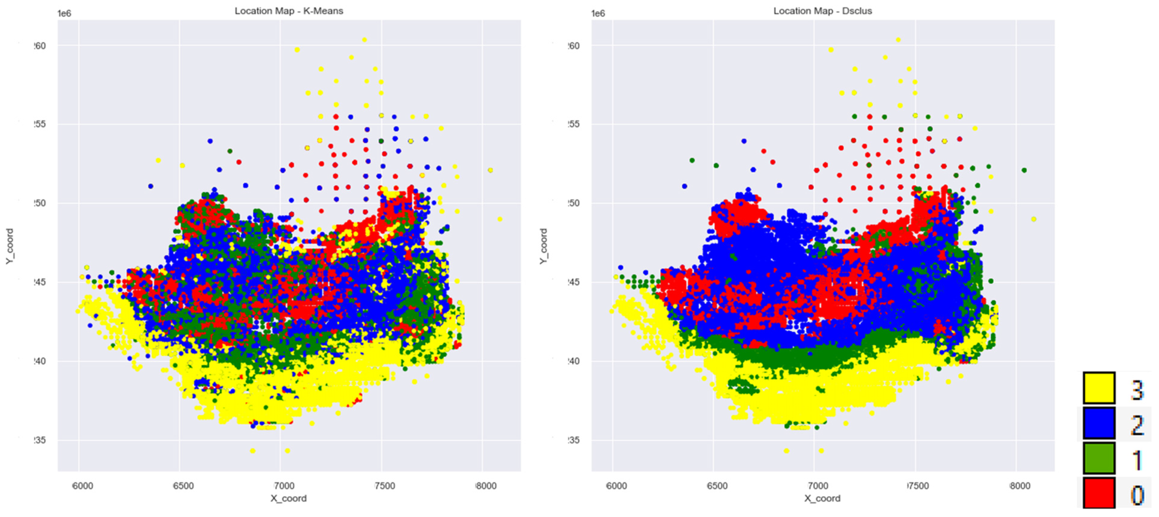
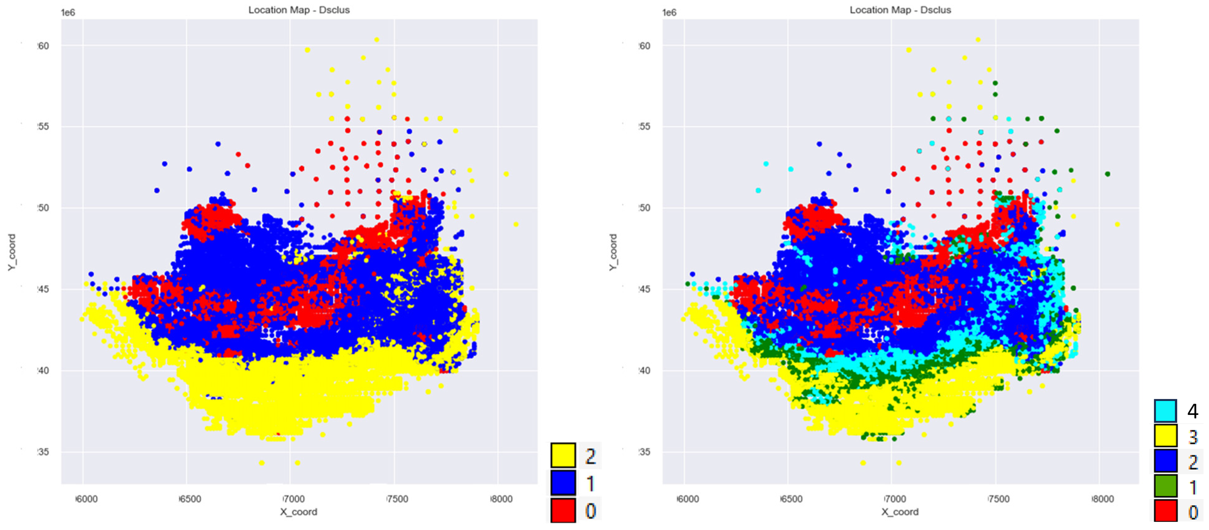
2.1.3. Dual-Space Clustering

The dual-space clustering technique, created by Martin and Boisvert in 2018, consists of three steps designed to provide a final cluster configuration with spatial structure. It starts by choosing a number (M) of nearest neighbors that will be evaluated. An initial sample is randomly chosen to start the process, and its M geographically closest samples are identified. Once the spatial neighbors are defined, the algorithm randomly selects a subset of them to form a mini-cluster by drawing a random number between 1 and M. To decide which samples will be selected, the squared Euclidean distance calculated in the multivariate space is used, favoring the most similar samples in terms of their variables. This process is repeated until all samples belong to a mini-cluster.
Next, all mini-clusters existent in the study area are evaluated and the most similar ones, in the multivariate space, are merged, regardless of whether they are not spatially near. The Ward’s method is employed in this step to merge the most similar clusters. This entire process is repeated multiple times, generating a different clustering configuration each time, due to the randomness involved in the mini-cluster formation.
Finally, all realizations and their results are saved in a matrix with N rows (where N is the number of samples) and L columns (where L is the number of times the process was repeated). Each cell in this matrix stores the cluster assignment for each sample. Then, a hierarchical clustering is applied to this matrix to extract the dominant configuration of the clusters, creating a similarity matrix (of size N × N) that counts how many times each sample was merged with the other samples, with this number being normalized by the number of realizations (L), providing a measure of the likelihood that each pair of samples belongs to the same cluster.

2.1.4. Spatial Autocorrelation

The spatial autocorrelation technique, developed by Scrucca in 2005, starts by choosing a critical distance value to define the relevant neighbors of a given data point. Then, the W matrix is created to store the following information: when the sample j is inside the critical distance from point i  w i j receives value 1, and when sample j is out of the critical distance from sample i, it receives value 0. This procedure defines the set of spatial neighbors for each sample, respecting the critical distance. Then, the local standardized Getis–Ord statistics (Equation (4)) is calculated for each sample i looking at its neighbor’s values:
z G i = j = 1 m w i j x j x ¯ w i s 2 m 1 m j = 1 m w i j 2 w i 2 ,  
where, m is the number of neighbors and j is the neighbors index, x ¯ = j = 1 m x j m is the mean value found in the neighborhood, s 2 = j = 1 m ( x j x ¯ ) 2 m is the standard deviation of the samples in the neighborhood and w i = j = 1 m w i j is the sum of all weigths in the neighborhood.
Positive values of the local standardized Getis–Ord statistics indicate that high values of evaluated variables surround the evaluated location, while negative values mean the opposite.
Formula (3) needs to be applied once for each variable in the database, so, if there are seven variables to be used as inputs in the cluster analysis, there will be seven Getis–Ord values, one for each variable. All those Getis–Ord values are then saved in a matrix Z, with N rows (representing the number of samples) and P columns (representing the number of variables). The K-Means technique is applied in the matrix Z, to extract the spatial clusters based on the multivariate spatial autocorrelation profiles.

2.1.5. Metrics to Evaluate the Ideal Number of Clusters

With the exception of hierarchical clustering, all other methods mentioned above demand that the user provide information about the desirable number of clusters that are to be generated. This information is usually not known, so a useful approach is to iteratively build scenarios by varying the number of clusters and then evaluating the results obtained. To help the user in this decision-making process, some metrics are available in the literature, such as Pseudo-F [33] and spatial entropy [31]. The former evaluates the clustering from a multivariate point of view and the last checks its spatial behavior, as explained below.
The Pseudo-F metric, represented in Equation (4), analyses the heterogeneity between clusters and the homogeneity within the cluster, and the higher the value obtained, the better:
P s e u d o   F = ( i = 1 k * n i ( x ¯ i . x ¯ ) ( x ¯ i . x ¯ ) ) / ( k * 1 ) ( i = 1 k * j = 1 n i ( x i j x ¯ i . ) ( x i j x ¯ i . ) ) / ( n k * ) ,
where the index i refers to the group (cluster) number, the index j is related to the sample number in the database, n is the number of samples, x ¯ i . is the mean vector of group i, x ¯ is the global mean vector, and k is the number of groups evaluated.
Spatial entropy, represented in Equation (5), measures the spatial structure of the clusters created, without considering any multivariate aspect:
H T o t a l = i = 1 N k = 1 K p i , k   l n   p i , k ,
where p i , k is the probability of finding a category k near to a local i, considering samples within a given search radius. The smaller the value found, the more homogeneously the clusters are distributed in space.
After choosing the best clustering algorithm and the ideal number of clusters, the next step is to ensure that the results have geological meaning. After geological validity is confirmed, the final part consists of interpolating the cluster’s labels through all 3D blocks in the model, amplifying the sample knowledge for the entire deposit. In this case study, this was achieved with the hierarchical indicator kriging.

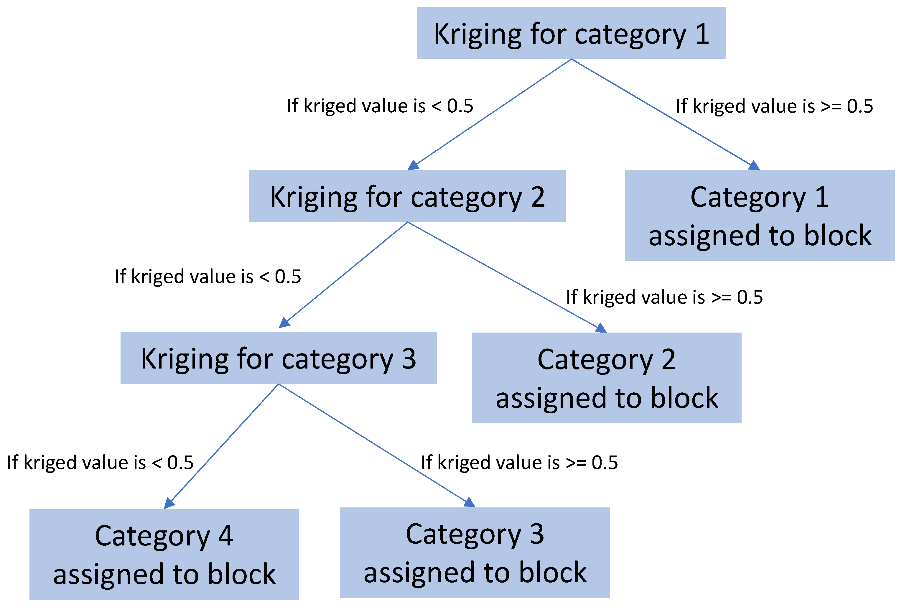
2.2. Hierarchical Indicator Kriging

Indicator kriging [34] is a technique used to provide, for each block in the 3D model, a probability of a given category to happen in such location. This category can reflect several aspects, as grades (probability of observing a Nb2O5 grade higher than 1% in one mining region), lithologies (probability of observing a bebedourite) or any other information able to be divided in two or more groups due to some criteria. The first step is to create the indicator variable, following the logic presented in Equation (6):
i u α ; k = 1 ,             i f   c a t e g o r y = k 0 ,             i f   c a t e g o r y k    
The sample positioned at location u α will receive a value of 1 if it belongs to category k and value 0 if it belongs to any other category.
After creating the indicator, the next step is to calculate the indicator variogram. Consider I u and I u + h , two values of a regionalized variable separated by a distance h. The variance between them is calculated using the variogram function 2 γ h , presented in Equation (7) [35]:
2 γ h = E I u I u + h 2 ,
where I u and I u + h are the values of the samples at positions u and ( u + h ) .
Subsequent to experimental variogram calculation, the next step is to fit a model to provide information about how, for any distance, the spatial correlation behaves. This variographic model is then used in the ordinary indicator kriging [36], to infer, for each block from the 3D block model, the probability of observing the category k in each location. The equation for the ordinary indicator kriging system is given by
p O K * u , k = α = 1 n λ α O K u , k i u α , k
where p O K u , k is the estimated probability of category k prevailing at the location u , λ α O K u , k represents the ordinary kriging weights for the indicator i u α , k , and n is the number of samples used in the estimation.
When only two categories exist, there is no need to krige both, once they are complementary. But when the number of indicators increase, additional care must be taken. Usually, when three or more indicators exists and are kriged, the probabilities obtained from them are evaluated and the block will receive the label corresponding to the indicator which returned the highest probability. Let us pose a hypothetical situation where the kriged probabilities are 0.26 for category 1, 0.20 for category 2, 0.14 for category 3, and 0.4 for category 4. Note that the most probable category is 4, but the probability of not observing category 4 in such location is 0.6 (the sum of all other categories), which is even higher than the probability of 4. So, to label a block using the highest probability is not always a good solution.
To solve this problem, an approach named hierarchical indicator kriging was created, and it is based on the following idea: instead of kriging all indicators and looking at all probabilities simultaneously to choose the highest, a hierarchical flow is created and one indicator is kriged against those that remain. For example, first, category 1 indicator is kriged. The probability value is evaluated: if it is higher or equal to 0.5, the category 1 label is assigned to that location, but if the probability is lower than 0.5, it means that there is a significant probability that the block does not belong to category 1. So, in case the block presents a low probability of belonging to category 1, it needs to pass through another round of kriging to evaluate to which category it will belong. Following this idea, it is natural to create a flowchart to organize the order of the categories that are to be estimated. An example is shown in Figure 1.
The hierarchical sequence or partitioning tree chosen for hierarchical indicator kriging (HIK) indeed affects the final modeling results. This is a highly relevant and often underestimated aspect of categorical geostatistical modeling. Understanding this influence requires an examination of both technical foundations and best practices from established methodologies.
A useful analogy comes from other geostatistical frameworks for categorical simulation, notably Truncated Gaussian Simulation [37] and Truncated PluriGaussian Simulation (TPGS) [38]. In these approaches, key modeling choices made by the geomodeller—such as the sequence of thresholds and how categories interact spatially—directly control the realizations.
Similarly, in the indicator kriging framework, including HIK, two key factors govern results: the sequence or structure of hierarchical splits and the definition of spatial trends, controlling local conditional probabilities for each category.
Recent studies confirm the critical role of hierarchy:
  • The authors of [39] demonstrate how different tree structures impact the realizations generated by Pluri-Gaussian Simulations. The authors state that building the tree structure for complex cases is not simple. The authors also emphasize that spatial and temporal relationships between different categories should be considered to build the tree.
  • The authors of [40] highlight that both Sequential Indicator Simulation (SIS) and HIK depend heavily on hierarchical decisions. Poorly defined hierarchies can lead to artifacts such as extreme weights or unrealistic spatial transitions.
  • The authors of [41] demonstrate that grouping similar rock types or materials in early hierarchical splits produces more geologically realistic boundaries, while poorly structured hierarchies compromise spatial continuity.
  • Insights from [42] regarding hierarchical Truncated Pluri-Gaussian models further emphasize that incorrect truncation trees—or by analogy, partitioning trees in HIK—negatively impact the spatial distribution and proportions of categories.
From a practical perspective, the hierarchy of HIK allows the geomodeller to incorporate their expertise. The traditional IK is not flexible, as all the categories are treated equally. On the contrary, the HIK can prioritize the most important categories by placing them early in the tree structure. Another possibility is to build the tree following the geological sequence of events. For instance, suppose that ore has been weathered. The HIK could model first the ore/waste boundary and later the boundary between the weathered and unweathered ore.
The hierarchical approach to building categorical models is not exclusive to the HIK algorithm. The authors of [43] show how a geological model of a copper deposit was built using interpretation of surfaces. The first step includes adding the surface of the mineralized sulfides. Then, the different types of sulfides are modeled. This hierarchical rationale is also used for reservoir modeling. In this case, geostatistical modeling typically begins by modeling the top and base surfaces of the reservoir. These two surfaces define one horizon of the reservoirs. Then, the facies within each horizon are modeled.

Best Practices for Hierarchy Definition in HIK

To ensure robust results, geomodellers typically apply intuitive and domain-informed rules to construct the hierarchy:
  • Start by splitting major geological or material groups, specifically those with the greatest dissimilarity in terms of physical properties, genesis, or economic value. Examples include
    Geotechnical modeling: dividing soft and hard rock;
    Mineral resource estimation: distinguishing ore from waste;
    Geometallurgical modeling: separating oxide ore from sulfide or primary ore.
  • After this first split, subsequent divisions progressively refine the hierarchy, ideally grouping categories with greater internal similarity at each stage. The process continues until each individual category or rock type is isolated.
This approach is supported by [44], who showed that hierarchies reflecting geological logic produce better results in habitat and categorical mapping, and that deeper, poorly conceived hierarchies can degrade model accuracy.
In essence,
  • Early splits influence large-scale spatial patterns;
  • Later splits refine finer-scale heterogeneity;
  • The order of splits governs how uncertainty and continuity propagate through the model, with different hierarchies producing distinct spatial realizations, even with identical input data.

2.3. Trend Model

In some situations, the proportions of classes and its indicators are not stationary. It is necessary to introduce an additional step during the modelling: trend model creation. The trend model is used to capture the long-range structure and separate it from the local fluctuations, making easier to model the variograms and represent the spatial structure of the phenomenon. Its use can provide some benefits such as avoiding abrupt transitions between categories (if they do not occur in reality), improving the probability’s accuracy in regions with lack of data, and introducing a specialist point of view in the modelling.
There are several ways of creating a trend model. The most common are vertical proportion curves (VPC [45]), the stochastic partial differential equation (SPDE [46]), adjusting a polynomial to infer the local proportion, and using the moving window average technique. The steps used to generate an estimate with a trend model are listed below:
(1)
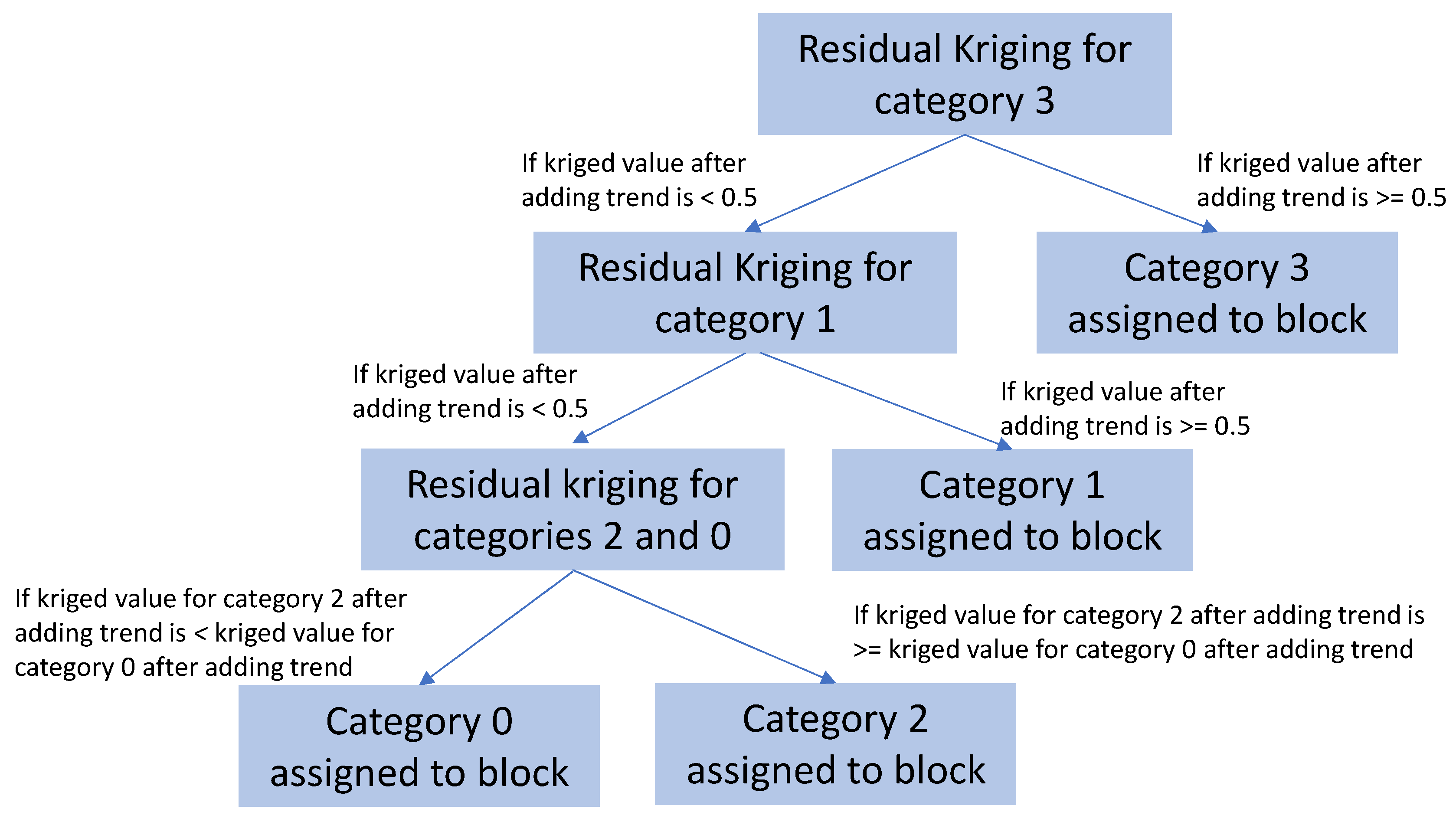
Build the trend model with an appropriate technique. Thus, for each block in the model, there will be a probability of belonging or not belonging to a category, given the block location;
(2)
Assign a trend value to each sample by migrating the trend from the closest block;
(3)
Subtract the category indicator from the migrated trend value to compute the residual for each sample;
(4)
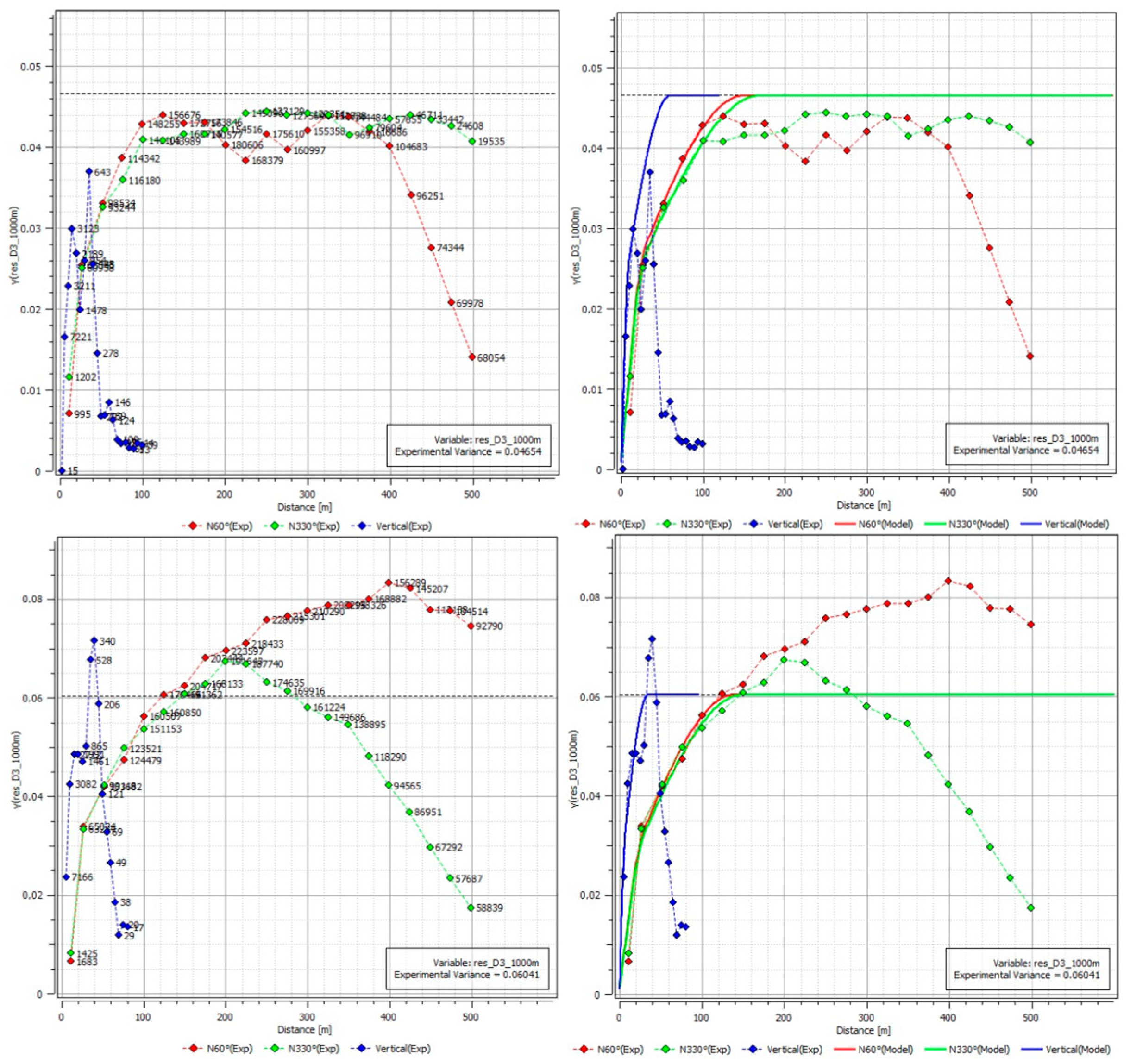
Build the residual variogram model;
(5)
Krige the residual or simulate it;
(6)
For each block, add the kriged (or simulated) residual to the trend value, ensuring the final probability remains within the 0 to 1 range;
(7)
Validate the results.

SPDE

Since the stochastic partial differential equation approach was selected to model the trend in this case study, some theorical background is provided next. For further details, the reader is referred to [46,47]. SPDE is a technique that allows the creation of a Gaussian random field to represent trends in a deposit. Combined with hierarchical indicator kriging (or other techniques), it helps to incorporate geological characteristics that are not easily modeled within traditional kriging workflows.
To fully comprehend this methodology, some key concepts need to be introduced. The first is the Matérn covariance function, presented in Equation (9):
C h = σ 2 2 1 ν Γ ν κ h ν K ν κ h ,
where σ 2 represents the a priori variance (sill); ν is the smoothness parameter, which controls the smoothness of the generated field (the higher its value, the smother the field); κ is a value related to the spatial range ( r a n g e   8 ν / κ , hence high κ values indicates small ranges and low κ values means the opposite); and K ν is the modified Bessel function of the second kind, which indicates how to covariance decays when the distance h increases. Note that, when the smoothness parameter is equal to 0.5, the Matérn model becomes the traditional exponential covariance model, and when it tends to infinite, it becomes a Gaussian model. Therefore, by using the Matérn covariance function, it is possible to define the spatial variability structure of the trend model created.
Then, a triangular mesh is created to cover the entire grid, presenting more data points where more information is available. Finally, the matrix representing the SPDE is built (Equation (10)) and the linear system is solved for each grid cell to achieve the trend model values.
κ 2 Δ α 2 x s = W s ,
where x s is the Gaussian random field created in point s; Δ is the Laplacian operator; α is a parameter related to the smoothness parameter ( α = ν + d / 2 , where d is the space dimension: 2 for 2D and 3 for 3D); and W(s) is Gaussian white noise.
In this study, the implementation of the SPDE was carried out using Isatis.neo® software (version 2024.04.2). Within the “Proportion Modeling” tool, the user can tune a hyperparameter named “Model vs. Data”, which controls the balance between honoring the samples and enforcing spatial smoothness in the trend model created. When its value is near zero, the trend model produces a less smooth map, once it needs to honor the data information. Conversely, when its value is close to one, the trend is smoother and less tightly constrained by data. The sill is automatically calculated from data; the user defines the range in the “Advanced Parameters” and the anisotropy orientation. For further details on the implementation, readers can refer to the software’s documentation.
The Isatis.neo® algorithm starts by creating an indicator variable for each category to convert the categorical information into probabilities for each block. These indicator variables are then transformed into Gaussian variables. The original problem with k categories is broken down into a sequence of binary comparisons following a hierarchical approach: category 1 is estimated against all others; then within the remaining group, category 2 is estimated against the rest; the process is repeated until only two categories remain. A Gaussian random field is constructed with SPDE at each step of this hierarchy, estimating the probability of observing one category against its complement. These binary probabilities are then combined through hierarchical multiplication to compute the final probability for each category in all blocks. This final procedure ensures that the probabilities for all categories sum to one.

3. Materials and Methods

3.1. Geological Aspects

The world’s largest niobium mineral deposits are associated with carbonatite alkaline intrusive rocks, with pyrochlore being the main niobium-bearing mineral. The Araxá niobium mine is related to the Barreiro Carbonatite Alkaline Complex, also known as the Araxá Carbonatite Alkaline Complex, and is recognized as the largest mineral resource and ore reserve of this substance. The main geological processes that formed the deposit were as follows:
Magmatism: Through the intrusion and evolution of a picritic magma and various liquid immiscibility processes, niobium naturally concentrated in the center of the intrusion, mainly associated with rocks from the petrogenetic series of phoscorites and dolomite carbonatite;
Hydrothermalism: Late fluid added more niobium to the primary mineralization and altered the magmatic-origin pyrochlore crystals, replacing calciopyrochlore with bariopyrochlore;
Tropical weathering: This process altered the carbonate and ferromagnesian minerals of the igneous rocks, leaching the mobile elements and generating a residual concentration of resistant minerals in the weathering zone. In addition to concentrating minerals of significant economic interest, this process also removed important contaminants (carbonates and micaceous minerals), enabling the development of a simplified, low-cost, and highly efficient mineral concentration route.
Other economically interesting substances are associated with this type of mineral deposit, such as phosphate (apatite), iron ore (magnetite), barite, titanium (anatase and ilmenite), and rare earth elements (monazite). Some of these substances are by-products of the pyrochlore and apatite concentration processes, such as magnetite and barite concentrates.

3.2. Processing Flowsheet

The processing plant consists of three main separation stages that strongly impact the resulting yield and pyrochlore recovery. These are desliming, magnetic separation and flotation. Magnetite, which occurs in the form of relatively large grains, is separated in low-intensity magnetic rotating drums. The desliming operation is achieved in a series of hydrocycloning stages after ball milling to reduce the particle sizes to a size that is suitable for efficient flotation concentration of pyrochlore. The flotation plant consists of a relatively complex circuit of rougher, cleaner and recleaner stages that are carried out in closed circuit with each other in order to maximize recovery at the required concentrate grade of Nb2O5.
Geometallurgical testing emulates the industrial plant well enough that it is possible to determine the quality of concentrate that can be achieved from a geometallurgical sample, and the associated yield and recovery.

3.3. Database Information

The database used in this study contains 26,080 samples isotopically analyzed for the following variables: Al2O3, Fe2O3, Nb2O5, P2O5 and SiO2 in the Run of Mine (ROM), yield, metallurgical recovery, magnetic yield, slimes yield, and Nb2O5 and P grades in the flotation concentrate. Due to the confidentiality requested by the company, more sensitive data such as grades and recovery cannot be shared throughout the text, so the boxplots presented in Figure 2 presents no y-axis numbers. However, this omission does not prevent the reader from understanding the methodology used and the results obtained. Figure 3 illustrates the sample positions in the deposit, with changes in the coordinates.

3.4. Cluster Analysis

The variables used as input for the cluster analysis have different magnitudes. For instance, P grades in flotation concentrate are typically at low levels, whereas the metallurgical recovery is usually very high. This disparity creates a challenge for cluster analysis once the variables with larger magnitudes tend to dominate the clustering process, overshadowing the variables with small values. To address this issue, a standard scaler was applied to the variables (Equation (11)), rescaling them with a mean equal to zero and a standard deviation of one.
Z i = x i x ¯ s ,  
where Z i is the standardized value for sample i, x i is the original value of sample i, and x ¯ and s are, respectively, the mean and the standard deviation of the variable across all samples in the dataset.
After standardizing the database, the next step was to proceed with the cluster analysis. Four techniques were employed in this case study: K-means, hierarchical clustering, dual-space clustering, and clustering by autocorrelation statistics, and the results obtained with each method were evaluated using Pseudo-F and spatial entropy metrics. Figure 4 illustrates the results obtained for these four techniques, for a number of clusters varying from 2 to 5.
The results obtained showed that, for any number of clusters selected, the K-Means technique (blue line) presented the best statistical results (summarized by the Pseudo-F metric). Analyzing the spatial entropy revealed a better spatial disposal of the clusters when dual-space clustering (red line) was used, for any number of clusters selected. Figure 5 shows the spatial distribution of the clusters generated when K-means and DSC were used. It is remarkable that dual-space clustering results more closely resemble the geological behavior expected, once high variability in short distances is not commonly observed. Those results highlight the spatial cluster techniques’ superiority in reproducing geological features, even though the multivariate statistical division of samples is not as accurate as the one obtained using K-means.
After choosing the technique, the next step was to decide the ideal number of clusters. This choice was made using the geological knowledge as the key pillar. It is known that adopting only two clusters would oversimplify the complex geology and metallurgical characteristics of the deposit. Dividing data into three domains (Figure 6, left) resulted in merging samples with high and low metallurgical recovery in the same cluster, which is undesirable. By choosing five clusters (Figure 6, right), no differences were perceived between clusters 3 and 4, with the Al2O3 grade in ROM being the only variable responsible for this split, which lacks geological/metallurgical relevance. Thus, it was decided to adopt the results with four clusters (the ones illustrated on the right side of Figure 5), once different metallurgical responses were observed in the groups and the spatial connectivity obtained was adequate for posterior modelling.
Figure 7 illustrates the variables’ boxplots by cluster. All variables were standardized to comply with the company’s confidentiality requirements, but this does not affect the validity of the conclusions. Cluster 0 (red) is highly magnetic and has a low percentage of slimes compared to the other clusters. Cluster 2 (blue) shows the highest mean metallurgical recovery and almost all of its samples achieve the target Nb2O5 grade in the concentrate (represented by 0.32 in the standardized scale). Geologically, the center zone, where clusters 0 and 2 are located, is predominated by dolomitic carbonatites with subordinated magnetites and phlogopites. Bebedourites and calcitic carbonatites are rarely found in this region. The high magnetic content observed in cluster 0 is probably related to the high presence of magnetites.
Cluster 3 (yellow) shows samples with a high percentage of slimes, low mean yield and recovery, and a high number of samples that are unable to achieve the concentration target grade, proving itself as the worse plant feed for the required product. Geologically, these samples belong to a lithological domain composed of silicate rocks from the bebedourite petrogenetic series and small bodies of calcitic carbonatites in the form of ring dikes.
Cluster 1 (green) also has a high percentage of samples which do not achieve the concentrate grade target, but its metallurgical recovery and yield are much better than the recoveries observed in cluster 3. This region is known to be a transition zone between the dolomitic carbonatites to the bebedourites, gradually increasing the presence of phlogopites.

3.5. Hierarchical Indicator Kriging

After defining each sample cluster, the next step was to interpolate this information for all blocks using hierarchical indicator kriging. The first action needed is to create the indicator variables following the logic presented in Equation (6).
Before beginning the variography and estimation process, there is a need to apply a trend model, once it is most probable to observe cluster 3 in the deposit edge and clusters 0 and 2 in the center, and the trend model can capture this regional tendency. Another valuable use of trend models is using them to incorporate qualitative information, as geological maps, aiming at using its information to increase model accuracy. In this case study, cluster 3 is geologically compatible with the bebedourite domain, which surrounds the deposit. It is important to ensure that the block model created reflects this characteristic. So, to better represent the geological features, it was decided to use the geological maps showing the bebedourite area in the trend model creation. This was achieved by the geology team, who created a grid of points over the area mapped as bebedourite and assigned these points a cluster label equal to 3. The information from data samples was then combined with these new points, and all of them were used to create the trend model with SPDE. This ensured that clusters 0, 1, or 2 did not appear in the bebedourite area, and, on the other hand, ensured that cluster 3 did not appear in the center, which is dominated by the dolomitic carbonatites. Figure 8 illustrates the bebedourite points mapped by the geology team, which are used as secondary information in the trend model.
To illustrate the results obtained without the trend model, Figure 9 shows the block model colored by the cluster when it was not used. The red lines show bebedourite regions mapped geologically, so cluster 3 should be estimated there. However, due to the proximity of samples which belong to clusters 0 and 1 the forecasts were made taking into account this information, erroneously predicting the cluster category and highlighting the importance of using a trend model.
After demonstrating the need to adopt a trend model in the estimate, the next step was to build it. The Isatis.neo® software (version 2024.04.2) was used for this task, and the hyperparameters were calibrated to produce a visual result that reflects the geological structure of the deposit. A “Model vs. Data” value of 0.5 was adopted, corresponding to intermediate smoothness. An isotropic ellipsoid was applied with 1000 × 1000 × 20 m dimensions. Thus, for each block, the probability of belonging to each cluster was calculated, as illustrated in Figure 10. After defining the trend probability for each block, it was necessary to define it for each sample in the database, which was done by merging the nearest block trend probabilities for the sample position. Then, the residual for each sample was calculated using the equation presented in (12). Figure 11 presents the flowsheet adopted in this study to assign to each block a cluster category.
r e s i d u a l u α ; k = i u α ; k t r e n d u α ; k
The experimental variograms for each residual variable were calculated and modelled, as illustrated in Figure 12 and Figure 13, and summarized in Table 1. To better capture the circular behavior observed in cluster 3, the deposit was divided into four quadrants. The NE-SW direction was modeled separately from the NW-SE direction to account for anisotropy.
Cross-validation was performed to ensure that the modeled variograms accurately capture the spatial continuity of the categorical variables. In this process, the residual variogram for category k was used in the cross-validation. The kriged results for each data point were then combined with the corresponding trend model for category k to estimate the probability of observing category k at that location. If the probability was greater than 0.5, the forecasted category for that point was assumed to be k; otherwise, if the probability was less than or equal to 0.5, the point was classified as not belonging to category k. Then, the forecast accuracy was calculated, resulting in the following values: 92.2% for category 0, 92.3% for category 1, 89.0% for category 2, and 96.3% for category 3.
The ellipsoids used had dimensions equal to the variogram range in all directions, minimum number of samples to perform kriging equal to two, eight angular sectors and six samples by sector.
It is important to remark that, after each residual kriging, the trend model built with SPDE needed to be added in each block, to check if the value obtained returned a probability equal or higher than 0.5, showing that the block had a significant probability of belonging to a given category. After going through the entire flowsheet, the validations were performed: the proportions of each category were checked to find consistency with the database, the swath plots were calculated, and the cross-validation was performed, together with a visual inspection of the results. Then, we identified the need to post-process the results due to the “salt and paper effect” in some regions. This was conducted using MAPS [48] and the results obtained can be visualized in Figure 14.

3.6. Mineralogical Interpretation of the Clusters

After defining the clusters and building their respective 3D models, the next step was to proceed with a complete mineralogical analysis to comprehend the characteristics of each one. For this, 45 drillhole samples were collected from cluster 0, 42 from cluster 1, 40 from cluster 2, and 47 from cluster 3. The samples by cluster were blended to create four representative samples of each cluster and were prepared according to the flowsheet explained in Section 3.2. A mineralogical analysis using XRD was then conducted on both the slimes and non-slime material, as well as on the magnetic and non-magnetic fractions. Using that information, the global mineralogy could be calculated by sample (Table 2).
Note that the highest metallurgical recovery observed in cluster 2 is related to the highest quantity of pyrochlore available in this area, combined with the reduced quantity of aluminophosphates, which notably impact the flotation due to interference in the process reagents and the slime coating effect. Cluster 0, which presented a high magnetic yield, shows an elevated quantity of magnetite, which easily explain this result. The high amount of barite in clusters 0 and 2 shows their importance in generating barite as a by-product, increasing mine profit, and making better use of the mineral resources available. Cluster 1 contains a high quantity of quartz and monazite, making this region important for observing rare earth elements. Cluster 3, which presented the worst process results, has elevated levels of goethite, magnetite, hematite, and aluminophosphates, combined with low quantities of pyrochlore, explaining the low recovery rates.

4. Conclusions

The geometallurgical domains built reflected critical geological features, widely related to the different performances observed when the materials are fed in the processing plant. Cluster 0 generates a significantly larger amount of magnetic material, which is explained by its high concentration of magnetite. Understanding this aspect is important when planning the deposition of this material in piles or studying the possibility of selling the magnetic concentrates as a by-product, bringing financial benefits to the company. Cluster 3 is marked by a small flotation yield and low recovery, which is very important information for mine planning to avoid long periods in which only this type of material is sent to the processing plant, resulting in a small volume of concentrate. This behavior is explained by the reduced quantity of pyrochlore available in this region, combined with high quantities of goethite, magnetite, hematite, and aluminophosphates. Cluster 2, which usually provides excellent metallurgical recovery and high yield, making it the best ore cluster, contains the highest amount of pyrochlore and reduced gangue minerals. Cluster 1 also presents a good metallurgical performance, but generates a slightly higher percentage of slimes compared to clusters 0 and 2.
The results obtained highlight the importance of understanding the performance of each cluster in the plant to optimize the use of available mineral resources, increase mine profitability, and reduce unexpected events during ore processing. The next steps in this study include developing a geometallurgical 3D model to quantify each geometallurgical variable block by block and conducting a complete review of the mine planning schedule to incorporate this information.

Author Contributions

Conceptualization, F.G.F.N.; Methodology, F.G.F.N.; Validation, J.F.C.L.C., R.M.A., L.N.C. and R.S.R.; Formal analysis, F.G.F.N.; Investigation, F.G.F.N., C.L.S. and R.S.R.; Resources, J.F.C.L.C.; Data curation, R.M.A.; Writing—original draft, F.G.F.N.; Writing—review & editing, J.F.C.L.C., C.L.S., R.M.A., L.N.C. and R.S.R.; Visualization, C.L.S.; Supervision, J.F.C.L.C. and L.N.C.; Project administration, J.F.C.L.C., R.M.A., L.N.C. and R.S.R.; Funding acquisition, J.F.C.L.C. and L.N.C. All authors have read and agreed to the published version of the manuscript.

Funding

This research was funded by Fundação Luiz Englert grant number 10163938652.

Data Availability Statement

As the data used in this study are confidential, they cannot be publicly disclosed or shared.

Conflicts of Interest

The authors Luciano Capponi, Rodrigo Alcântara and Rafael Souza are employed by CBMM (Companhia Brasileira de Metalurgia e Mineração), which provided access to the data used in this study. The company had no influence on the interpretation or publication of the results. The authors Fernanda Niquini, João Felipe Costa and Claudio Schneider received a post-doctoral fellowship from Fundação Luiz Englert to support this research. The funding agency had no role in the design, execution, or publication of the study.

References

  1. Niquini, F.G.F.; Costa, J.F.C.L.; Schneider, C.L.; Pereira, M.A.S. Economical definition of ore: Grade cutoffs or geo metallurgical response? In Proceedings of the 12th International Geostatistics Congress, Ponta Delgada, Portugal, 2–6 September 2024. [Google Scholar]
  2. Lemos, M.G.; Valente, T.; Marinho-Reis, A.P.; Fonseca, R.; Dumont, J.M.; Ferreira, G.M.M.; Delbem, I.D. Geoenvironmental study of gold mining tailings in a circular economy context: Santa Barbara, Minas Gerais, Brazil. Mine Water Environ. 2021, 40, 257–269. [Google Scholar] [CrossRef]
  3. Lemos, M.G.; Valente, T.M.; Reis, A.P.M.; Fonseca, R.M.F.; Guabiroba, F.; Mata Filho, J.G.; Magalhães, M.F.; Delbem, I.D.; Diório, G.R. Adding value to mine waste through recovery of Au, Sb, and As: The case of auriferous tailings in the Iron Quadrangle, Brazil. Minerals 2023, 13, 863. [Google Scholar] [CrossRef]
  4. Louwrens, E.; Napier-Munn, T.; Keeney, L. Geometallurgical characterisation of a tailings storage facility—A novel approach. In Proceedings of the Tailings and Mine Waste Management for the 21st Century, Sydney, NSW, Australia, 27–28 July 2015. [Google Scholar]
  5. Knight, R.; Olson Hoal, K.; Abraham, A.P.G. Three-dimensional geometallurgical data integration for predicting concentrate quality and tailings composition in a massive sulfide deposit. In Proceedings of the First AUSIMM International Geometallurgy Conference, Brisbane, QLD, Australia, 5–7 September 2011; pp. 227–232. [Google Scholar]
  6. Niquini, F.G.F.; Branches, A.M.B.; Costa, J.F.C.L.; Moreira, G.d.C.; Schneider, C.L.; de Araújo, F.C.; Capponi, L.N. Recursive feature elimination and neural networks applied to the forecast of mass and metallurgical recoveries in a Brazilian phosphate mine. Minerals 2023, 13, 748. [Google Scholar] [CrossRef]
  7. Niquini, F.G.F.; Costa, J.F.C.L. Mass and Metallurgical Balance Forecast for a Zinc Processing Plant Using Artificial Neural Networks. Nat. Resour. Res. 2020, 29, 3569–3580. [Google Scholar] [CrossRef]
  8. Boisvert, J.B.; Rossi, M.E.; Ehrig, K.; Deutsch, C.V. Geometallurgical modeling at Olympic Dam Mine, South Australia. Math. Geosci. 2013, 45, 901–925. [Google Scholar] [CrossRef]
  9. Montoya, P.A.; Keeney, L.; Jahoda, R.; Hunt, J.; Berry, R.; Drews, U.; Chamberlain, V.; Leichliter, S. Techniques applicable to prefeasibility projects—La Colosa case study. In Proceedings of the First AUSIMM International Geometallurgy Conference, Brisbane, QLD, Australia, 5–7 September 2011; pp. 103–111. [Google Scholar]
  10. Niquini, F.G.F.; Andrade, I.A.; Costa, J.F.C.L.; Silva, V.M.; Marcelino, R.S. A workflow to create geometallurgical clusters without looking directly at geometallurgical variables. Miner. Eng. 2025, 222, 109171. [Google Scholar] [CrossRef]
  11. Faouzi, R.; Oumesaoud, H.; Naji, K.; Benzakour, I.; Aboulhassan, M.A.; Faqir, H.; Tahari, H. Predictive geometallurgical modeling for flotation performance in mixed copper ores using discriminatory methods. Arab. J. Sci. Eng. 2024, 49, 8057–8078. [Google Scholar] [CrossRef]
  12. Siddiqui, M.U.; Erwin, K.; Khan, S.; Chandramohan, R.; Meinke, C. An efficient sample selection methodology for a geometallurgy study utilizing statistical analysis techniques. Min. Metall. Explor. 2024, 41, 2193–2201. [Google Scholar] [CrossRef]
  13. Mu, Y.; Salas, J.C. Data-driven synthesis of a geometallurgical model for a copper deposit. Processes 2023, 11, 1775. [Google Scholar] [CrossRef]
  14. Bhuiyan, M.; Esmaieli, K.; Ordóñez-Calderón, J.C. Application of data analytics techniques to establish geometallurgical relationships to bond work index at the Paracutu Mine, Minas Gerais, Brazil. Minerals 2019, 9, 302. [Google Scholar] [CrossRef]
  15. Rajabinasab, B.; Asghari, O. Geometallurgical domaining by cluster analysis: Iron ore deposit case study. Nat. Resour. Res. 2018, 28, 665–684. [Google Scholar] [CrossRef]
  16. Sepúlveda, E.; Dowd, P.A.; Xu, C. Fuzzy clustering with spatial correction and its application to geometallurgical domaining. Math. Geosci. 2018, 50, 895–928. [Google Scholar] [CrossRef]
  17. Manfrino, A. Unravelling the factors impacting on concentrate quality by geometallurgical data analysis at Fortescue Metals Group’s Iron Bridge Magnetite Mine. In Proceedings of the Iron Ore Conference 2015, Perth, WA, Australia, 13–15 July 2015; pp. 567–578. [Google Scholar]
  18. Romary, T.; Rivoirard, J.; Deraisme, J.; Quinones, C.; Freulon, X. Domaining by Clustering Multivariate Geostatistical Data. In Geostatistics Oslo 2012. Quantitative Geology and Geostatistics; Abrahamsen, P., Hauge, R., Kolbjørnsen, O., Eds.; Springer: Dordrecht, The Netherlands, 2012; Volume 17. [Google Scholar] [CrossRef]
  19. Rolo, R.M.; Moreira, G.; Guimarães, O.R.A.; Fonseca, C.; Usero, G. Machine learning driven domain modeling for stratigraphic deposits. In Proceedings of the APCOM 2023, Rapid City, SD, USA, 25–28 June 2023. [Google Scholar]
  20. Moreira, G.C.; Costa, J.F.C.L.; Marques, D.M. Defining geologic domains using cluster analysis and indicator correlograms: A phosphate-titanium case study. Appl. Earth Sci. 2020, 129, 176–190. [Google Scholar] [CrossRef]
  21. Koruk, K.; Ortiz, J.M. Geological Domaining with Unsupervised Clustering and Ensemble Support Vector Classification. Min. Metall. Explor. 2023, 40, 2537–2549. [Google Scholar] [CrossRef]
  22. Madani, N.; Maleki, M.; Sepidbar, F. Application of geostatistical hierarchical clustering for geochemical population identification in Bondar Hanza copper porphyry deposit. Geochemistry 2021, 81, 125794. [Google Scholar] [CrossRef]
  23. Hong, J.; Oh, S. Model Selection for Mineral Resource Assessment Considering Geological and Grade Uncertainties: Application of Multiple-Point Geostatistics and a Cluster Analysis to an Iron Deposit. Nat. Resour. Res. 2021, 30, 2047–2065. [Google Scholar] [CrossRef]
  24. Scheidt, C.; Caers, J. Representing Spatial Uncertainty Using Distances and Kernels. Math. Geosci. 2009, 41, 397–419. [Google Scholar] [CrossRef]
  25. Okada, R.; Costa, J.F.C.L.; Rodrigues, Á.L.; Kuckartz, B.T.; Marques, D.M. Scenario reduction using machine learning techniques applied to conditional geostatistical simulation. REM—Int. Eng. J. 2019, 72, 63–68. [Google Scholar] [CrossRef]
  26. Bye, A.R. Case studies demonstrating value from geometallurgy initiatives. In Proceedings of the GeoMet 2011: The First AusIMM International Geometallurgy Conference 2011, Brisbane, QLD, Australia, 5–11 September 2011; AusIMM Australasian Institute of Mining and Metallurgy: Carlton, VIC, Australia, 2011. [Google Scholar]
  27. Leal, R.S.; Peroni, R.L.; Costa, J.F.C.L.; Pereira, S.G.; Martins, R.M.; Capponi, L.N. Geostatistics applied to geometallurgical modeling. In Proceedings of the 24th World Mining Congress PROCEEDINGS, Rio de Janeiro, Brazil, 18–21 October 2016; IBRAM: Rio de Janeiro, Brazil, 2016. [Google Scholar]
  28. Vieira, M.; Costa, J.F.C.L. Geometallurgical modelling to help in predicting zinc metallurgical recovery. In Proceedings of the 24th World Mining Congress PROCEEDINGS, Rio de Janeiro, Brazil, 18–21 October 2016; IBRAM: Rio de Janeiro, Brazil, 2016. [Google Scholar]
  29. Sokal, R.R.; Sneath, P.H.A. Principles of Numerical Taxonomy; W. H. Freeman: New York, NY, USA, 1963. [Google Scholar]
  30. MacQueen, J. Some methods for classification and analysis of multivariate observations. In Proceedings of the Fifth Berkeley Symposium on Mathematical Statistics and Probability, Oakland, CA, USA, 21 June–18 July 1965; Volume 1, pp. 281–297. [Google Scholar]
  31. Martin, R.; Boisvert, J. Towards justifying unsupervised stationary decisions for geostatistical modeling: Ensemble spatial and multivariate clustering with geomodeling-specific clustering metrics. Comput. Geosci. 2018, 120, 82–96. [Google Scholar] [CrossRef]
  32. Scrucca, L. Clustering multivariate spatial data based on local measures of spatial autocorrelation. Quad. Dip. Econ. Finanz. Stat. Univ. Perugia 2005, 20, 11. [Google Scholar]
  33. Calinski, T.; Harabasz, J. A dendrite method for cluster analysis. Commun. Stat.—Theory Methods 1974, 3, 1–27. [Google Scholar] [CrossRef]
  34. Journel, A.G. The indicator approach to estimation of spatial data. In Proceedings of the 17th APCOM, New York, NY, USA, 9–22 April 1982; Port City Press: New York, NY, USA, 1982; pp. 793–806. [Google Scholar]
  35. Journel, A.G.; Huijbregts, C.J. Mining Geostatistics; Academic Press: London, UK, 1978; 600p. [Google Scholar]
  36. Goovaerts, P. Geostatistics for Natural Resources Evaluation; Oxford University Press: New York, NY, USA, 1997; 483p. [Google Scholar]
  37. Matheron, G. The Theory of Regionalized Variables and Its Applications; École des Mines de Paris: Paris, France, 1971; 211p. [Google Scholar]
  38. Armstrong, M.; Galli, A.; Beucher, H.; Le Loc’h, G.; Renard, D.; Doligez, B.; Eschard, R.; Geffroy, F. Plurigaussian Simulation in Geosciences, 2nd ed.; Springer: Berlin, Germany, 2011; 182p. [Google Scholar]
  39. Sektnan, A.; Vázquez, A.A.; Hauge, R.; Aarnes, I.; Skauvold, J.; Vevle, M.L. A Tree Representation of Pluri-Gaussian Truncation Rules. Math. Geosci. 2025, 57, 445–470. [Google Scholar] [CrossRef]
  40. Ortiz, R.B. Advances in Geostatistical Modeling of Categorical Variables. Master’s Thesis, University of Alberta, Edmonton, AB, Canada, 2024. [Google Scholar]
  41. Amarante, F.A.N.; Rolo, R.M. Boundary simulation–a hierarchical approach for multiple categories. Appl. Earth Sci. 2021, 130, 123–135. [Google Scholar] [CrossRef]
  42. Sanchez, H.V. Truncation Trees in Hierarchical Truncated PluriGaussian Simulation. Master’s Thesis, University of Alberta, Edmonton, AB, Canada, 2023. [Google Scholar]
  43. Rossi, M.E.; Deutsch, C.V. Mineral Resource Estimation; Springer Science & Business Media: Berlin, Germany, 2013; 332p. [Google Scholar]
  44. Porskamp, P.; Rattray, A.; Young, M.; Ierodiaconou, D. Multiscale and hierarchical classification for benthic habitat mapping. Geosciences 2018, 8, 119. [Google Scholar] [CrossRef]
  45. Volpi, B.; Galli, A.; Ravenne, C. Vertical proportion curves: A qualitative and quantitative tool for reservoir characterization. In Proceedings of the First Latin American Congress of Sedimentology, Isla de Margarita, Venezuela, 16–19 November 1997. [Google Scholar]
  46. Carrizo Vergara, R.; Allard, D.; Desassis, N. A general framework for SPDE-based stationary random fields. Bernoulli 2022, 28, 1–32. [Google Scholar] [CrossRef]
  47. Lindgren, F.; Rue, H.; Lindström, J. An Explicit Link between Gaussian Fields and Gaussian Markov Random Fields: The Stochastic Partial Differential Equation Approach. J. R. Stat. Soc. Ser. B Stat. Methodol. 2011, 73, 423–498. [Google Scholar] [CrossRef]
  48. Deutsch, C.V. Cleaning categorical variable (lithofacies) realizations with maximum a-posteriori selection. Comput. Geosci. 1998, 24, 551–562. [Google Scholar] [CrossRef]
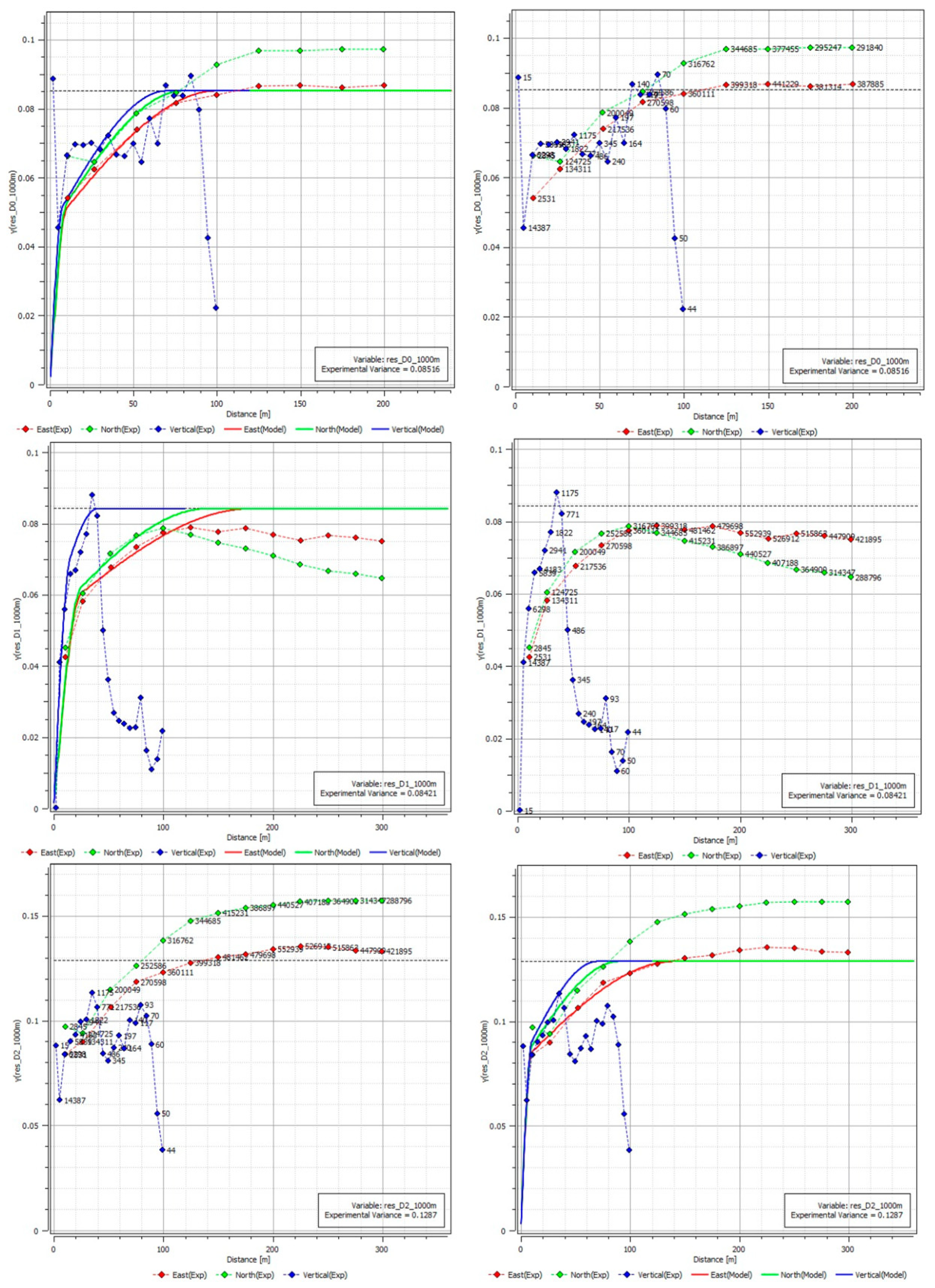
Figure 1. Example of a flowchart used to organize the sequence of krigings.
Minerals 15 00755 g001
Figure 2. Boxplots of the input variables used in the cluster analysis. Some variables present high variability (e.g., recovery, Fe2O3 grade in ROM), while others exhibit low dispersion (e.g., P in concentrate, Nb2O5 in ROM).
Minerals 15 00755 g002
Figure 3. Samples distribution in the deposit. The colors indicate the yield of each sample, with warmer colors representing higher yields and cooler colors representing lower yields. Due to the confidentiality requirements of the data provider, absolute values cannot be disclosed.
Minerals 15 00755 g003
Figure 4. Pseudo-F (left) and spatial entropy (right) for different number of clusters and different clustering techniques.
Minerals 15 00755 g004
Figure 5. Spatial distribution obtained when K-means (left) and DSC (right) algorithms were used to divide the samples into four clusters. The colors represent the different clusters generated by each methodology.
Minerals 15 00755 g005
Figure 6. Scenario with three (left) and five (right) clusters generated with the dual-space clustering algorithm. The colors represent the three clusters generated by DSC in the left image and the five clusters generated by DSC in the right image.
Minerals 15 00755 g006
Figure 7. Input variables boxplots colored by cluster.
Minerals 15 00755 g007
Figure 8. Bebedourite mapped geologically at the edge of the deposit.
Minerals 15 00755 g008
Figure 9. Block model colored by cluster when the trend model is not used to delimit the cluster 3 area.
Minerals 15 00755 g009
Figure 10. Trend model created with SPDE, showing the probability of belonging to each cluster.
Minerals 15 00755 g010
Figure 11. Flowsheet used for hierarchical indicator kriging.
Minerals 15 00755 g011
Figure 12. Experimental variograms and variogram models adjusted to the residual of cluster 0 (first row), cluster 1 (second row), and cluster 2 (third row).
Minerals 15 00755 g012
Figure 13. Experimental variograms and variogram models adjusted to the residual of cluster 3 in NE/SW direction (first row), and cluster 3 in the NW/SE direction (second row).
Minerals 15 00755 g013
Figure 14. Vertical section (Z = 1067.6 m) showing the results before (left) and after (right) MAPS post-processing was applied (Z = 1067.6 m).
Minerals 15 00755 g014
Table 1. Variogram model parameters.
VariableAnisotropy RotationNugget Effect1st StructureRange 1st StructureSill 1st Structure2nd StructureRange 2nd StructureSill 2nd Structure
Residual - Cluster 0D0° N90° p90°0Spherical10/10/7.5 m0.05Spherical100/80/70 m0.04
Residual - Cluster 1D0° N90° p90°0Spherical25/25/15 m0.05Spherical180/140/40 m0.03
Residual - Cluster 2D0° N90° p90°0Spherical10/10/10 m0.08Spherical140/90/70 m0.05
Residual - Cluster 3 NW-SED0° N60° p90°0Spherical30/30/10 m0.02Spherical150/170/60 m0.03
Residual - Cluster 3 NE-SWD0° N60° p90°0Spherical30/30/7.5 m0.02Spherical140/150/35 m0.04
Table 2. Global mineralogy (%) by cluster.
MineralCluster 0Cluster 1Cluster 2Cluster 3
Pyrochlore3.134.084.851.47
Barite16.526.4225.143.21
Goethite28.5439.8630.8838.71
Hematite20.539.9012.9916.54
Magnetite12.673.518.5318.64
Aluminophosphates3.367.542.298.94
Clay minerals2.074.082.842.36
Titanium oxide2.212.632.291.33
Monazite3.514.113.592.48
Quartz4.7415.604.602.91
Hollandite1.311.981.500.94
Disclaimer/Publisher’s Note: The statements, opinions and data contained in all publications are solely those of the individual author(s) and contributor(s) and not of MDPI and/or the editor(s). MDPI and/or the editor(s) disclaim responsibility for any injury to people or property resulting from any ideas, methods, instructions or products referred to in the content.

