Multi-Seam Coal Deposit Modeling via Principal Component Analysis & GIS

Abstract

Spatial modeling and evaluation is a critical step for planning the exploitation of mineral deposits. In this work, a methodology for the investigation of a multi-seam coal deposit spatial variability is proposed. The study area includes the Klidi (Florina, Greece) multi-seam lignite deposit which is suitable for surface mining. The analysis is based on the original data of 76 exploratory drill-holes in an area of 10 km², in conjunction with the geological and geomorphological data of the deposit. The analytical methods include drill-hole data analysis and evaluation based on an appropriate algorithm, principal component analysis and geographic information techniques. The results proved to be very satisfactory for the explanation of the maximum variance of the initial data values as well as the identification of the deposit structure and the optimum planning of mine development. The proposed analysis can be also helpful for minimizing cost and optimizing efficiency of surface mining operations. Furthermore, the provided methods could be applied in other areas of geosciences, indicating the theoretical value as well as the important practical implications of the analysis.

1. Introduction

Coal deposit modeling and evaluation as well as the process of mineable reserves estimation are essential and very important aspects of mine planning. In this framework, the modeling and evaluation procedure for the estimation of mineable reserves of multi-seam coal deposits could be divided into three main stages: (1) geologic modeling, (2) spatial block modeling, and (3) estimation of mineable lignite reserves [1]. Considering the spatial modeling of the deposits, quantitative understanding of the spatial variability of coal energy reserves helps to optimize mine exploitation and to reduce fluctuations in the quality of the fuel supplied to power plants [2].

There are mining industry accepted methods for splitting a coal deposit into mine development sectors and optimizing the mine planning and design. The main issue is to optimize the mining operations that usually refer to the application of operations research models [3,4]. Although the three-dimensional description of the deposit is helpful for modeling purposes, its computational complexity is not easily handled. In addition, a primary segmentation of the deposit into sectors, according to quantitative and qualitative criteria, is usually desirable for mine planning and design purposes. The primary factor for such a segmentation is the tectonic structure of the deposit that mainly defines regions of different geometry. Based on drill-hole data, conventional methods including cross sections and contour maps of the quantitative and qualitative variables within each tectonic region could provide deposit segmentation, especially in deposits with horizontal layers. However, these methods are not adequate for coal deposits with a complicated structure.

In an attempt to address the topic of multi-seam coal deposit spatial modeling and evaluation in a contemporary and sufficient way, this research work proposes and presents the coupling of principal component analysis (PCA) and geographic information system (GIS) techniques.

PCA is a statistical method for reducing the dimensions of complex datasets, increasing interpretability, while at the same time minimizing information loss [5]. In simpler words, it is used for converting a complex dataset of possibly correlated variables into a smaller collection of uncorrelated factors (known as principal components) that contain most of the information of the initial dataset.

In an integrated decision-making model, Roumpos et al. [6] considered the main factors that influence the evaluation of a lignite deposit and the optimization of a combined project of mine exploitation and power plant operation for electricity generation. The application of the proposed model showed that the mineral deposit factor which is related to the deposit data in combination with the mining characteristics has a particular effect on the viability of the project.

Spatial analysis of deposit indicators, combined with GIS applications, can provide a useful tool for evaluating a coal deposit in the framework of the corresponding surface mine investment analysis [7]. Furthermore, spatial analysis of coal energy reserves for exploitation planning and quality control can resolve variations of various properties at different scales and identify potentially useful correlations between variables [2]. The determination of the geological and spatial variability of the parameters that affect initial planning and final mine design is an essential part of mine modeling. It also affects the strategic mine exploitation sequence, from the opening up of the mine to the end of its life [4].

Statistics, and more specifically; geostatistics, are effective approaches to analyze mineral deposit parameters and to provide tools for evaluating mining processes, covering all aspects of the exploitation, from the preliminary pre-mining deposit research to the post-mining reclamation works. Recent examples of the previous arguments are the works of Lishchuk et al. [8] and Carvalho and Dimitrakopoulos [9]. The first paper deals with the construction of a “synthetic ore body model”, for simulating a mining value chain for data integration, by using a synthetic deposit, mine production, constrained by a mine plan, and a simulated beneficiation process. The second one incorporates geostatistical simulations with other techniques in an attempt to optimizing mining complexes operations.

Closer to the present paper is the work of Bhuiyan et al. [10], where data analysis techniques (including the PCA method) are applied, for establishing relationships between the Bond Work Index (BWI) and geomechanical, geophysical and geochemical variables for the Paracatu gold orebody in Brazil.

PCA has been applied in several cases as a useful geostatistical modeling tool [11] and for different purposes. For example, PCA has been applied in hydrochemistry data acquisition [12,13], in geotechnical properties of formations data [14], in quality composition of geological formations and trace elements data [15], etc. PCA is also implemented in various topics concerning mining activities and their impacts, especially coal mining, mainly regarding environmental and quality aspects [16,17,18,19,20,21].

According to Dowd et al. [22], modeling, estimation and simulation of geometallurgical variables and their integration into resource and reserve estimation and mine planning present challenges during strategic mine planning and design.

The identification of the surface mining regions of certain economic importance considering physicochemical or geometrical characteristics of a multi-seam coal deposit, based on the available drill-hole data and geostatistical techniques, is an interesting research topic. Taking into account the large number of parameters, which are related to coal deposits for surface mine development, geostatistical modeling should be applied for the analysis of the large datasets derived from the primary deposit drill-hole survey.

The objective of this paper is to incorporate PCA and GIS modeling of a multi-seam coal deposit into the mine planning and design model for the development of a surface coal mine. Emphasis is placed on the segmentation of the deposit into sectors of different technical and economic characteristics for further mine planning and design purposes. In short, the main goal of this research is to present and test a new method for mine planning and development of multi-seam coal deposits.

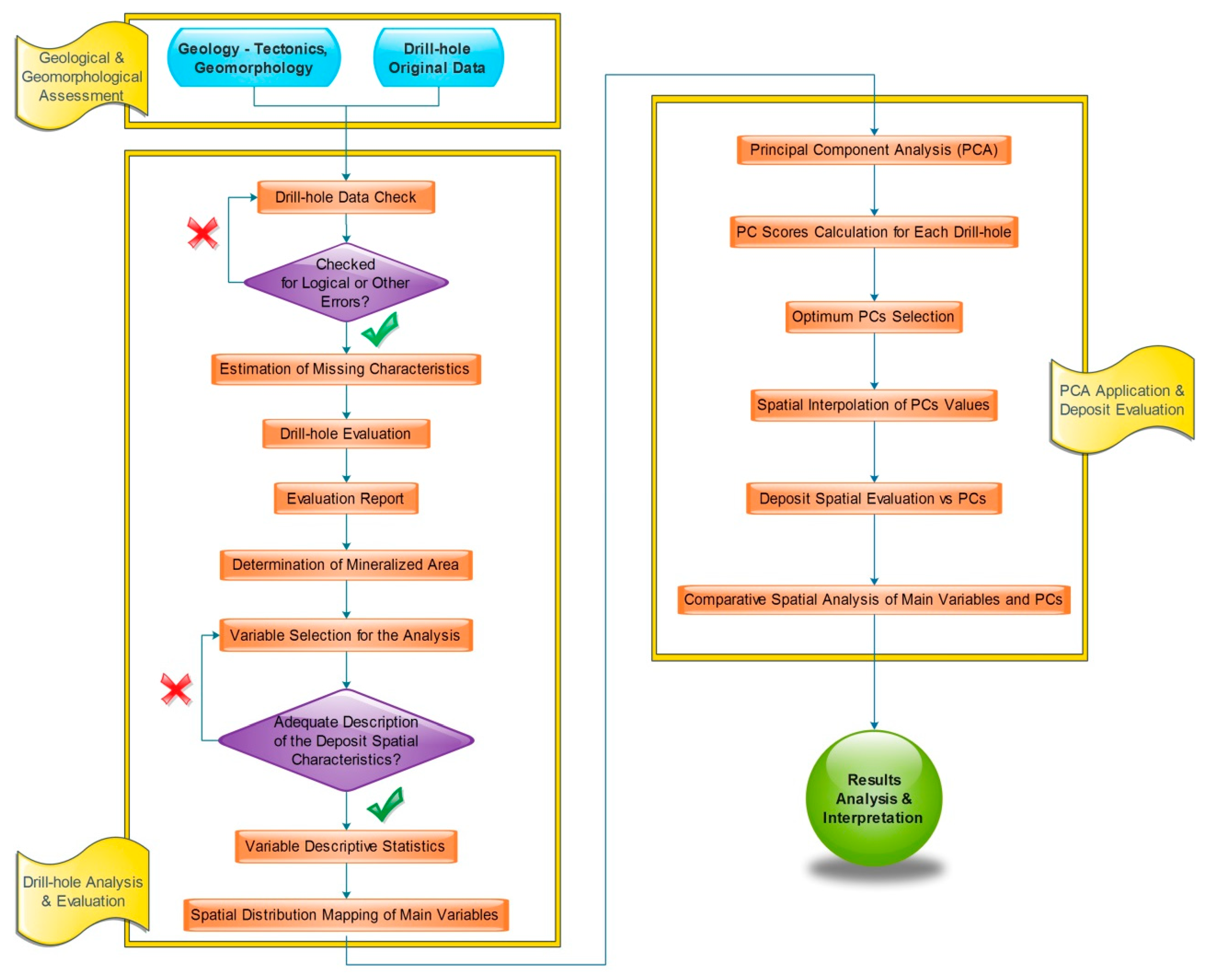
Figure 1 shows the flowchart of the research steps considering a multi-seam coal deposit, with frequently changing sequences of coal and waste layers.

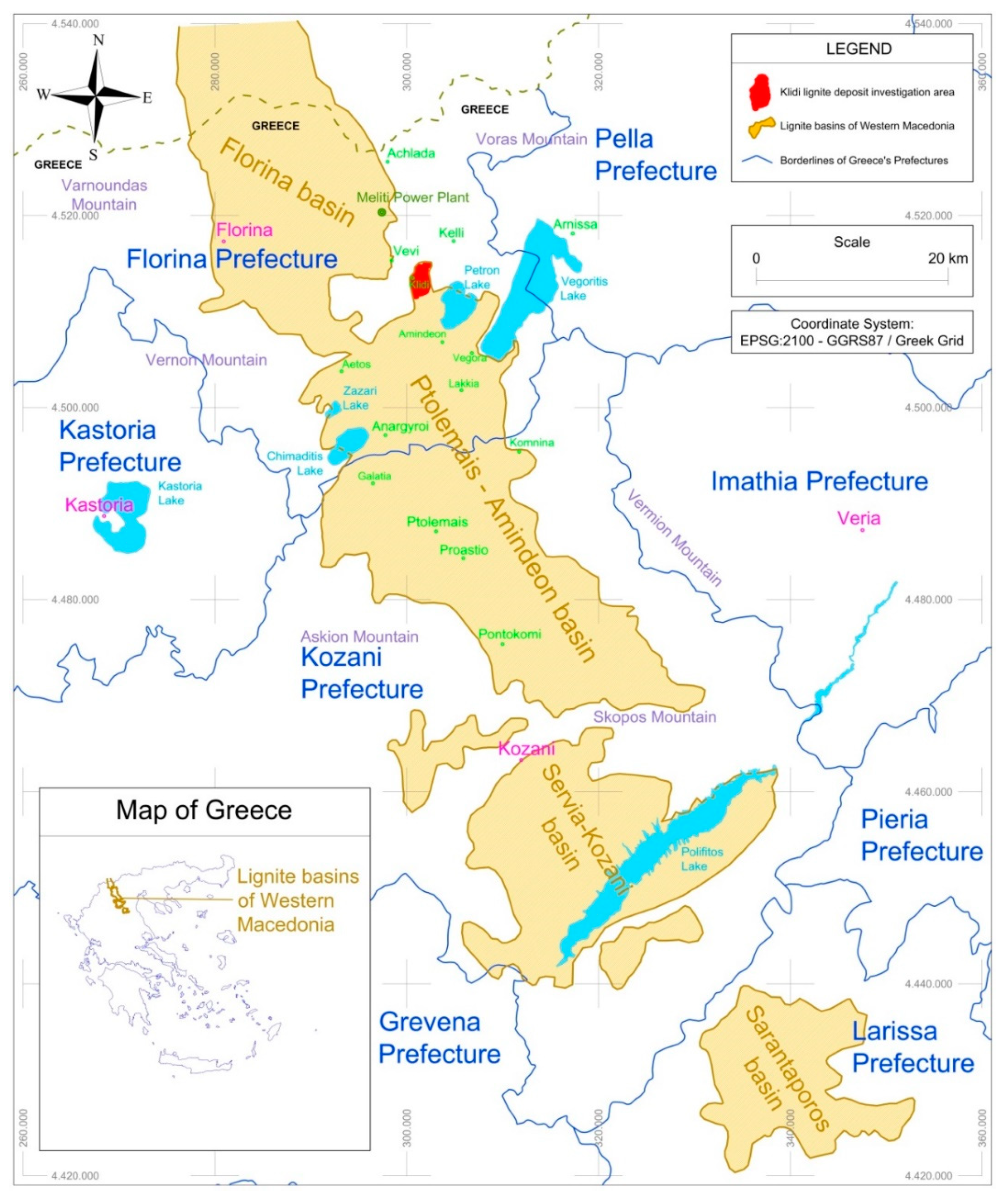
The methodology presented in this paper is applied to the Klidi lignite mining field, in the Northern part of Greece (West Macedonia) and specifically in the tectonic basin that extends along the axis Florina–Ptolemais–Kozani (Figure 2). Specifically, it is located in the eastern-southeastern boundary of the entire Florina mining area, approximately 22 km east–southeast of the city of Florina. It extends approximately 3 km N–S and approximately 1.7 km E–W (Figure 2).

This work provides the framework for a better understanding of multi-seam deposit characteristics and set solid directions for optimum mine exploitation planning. As will be discussed in the following sections, the applied analysis was justified by the results, which proved to be very useful, not only for establishing the foundations for the identification of the deposit structure and the optimum planning of mine development, but also for validating the methodological approach itself.

2. Coal Deposit Setting

Lignite is a type of low-rank coal, which is deposited on earth’s higher stratigraphic layers. Lignite is of particular significance for the power-generating branch of Greece as it covers about 30% of its electricity generation needs. The confirmed lignite reserves of Greece amount to 3.5 billion tons, out of which 2.3 billion tons (66%) are economically recoverable reserves. These reserves are distributed in various regions of Greece [23]. The vast majority of Greek lignite deposits are located in the Northern part of Greece (West Macedonia) and specifically in the tectonic basin that extends along the axis Florina–Ptolemais–Kozani (Figure 1). The geological formation of Greek deposits is developed on many horizontal seams of small and changing thickness, alternating with intermediate waste beds of different lithological and petrographic content.

The Klidi mining area is hilly with surface elevations ranging between +750 m and +1100 m above sea level (a.s.l.). The area of the planned mine covers approximately 6 km², including the Klidi village in the west of the field [24]. The lignite basin of the deposit progressively broadens from NW to SE with a decrease of surface altitudes. The mine is planned to contribute to the lignite demand of the 330 MW Meliti Power Plant, which is located 13 km NW from the mine (road distance).

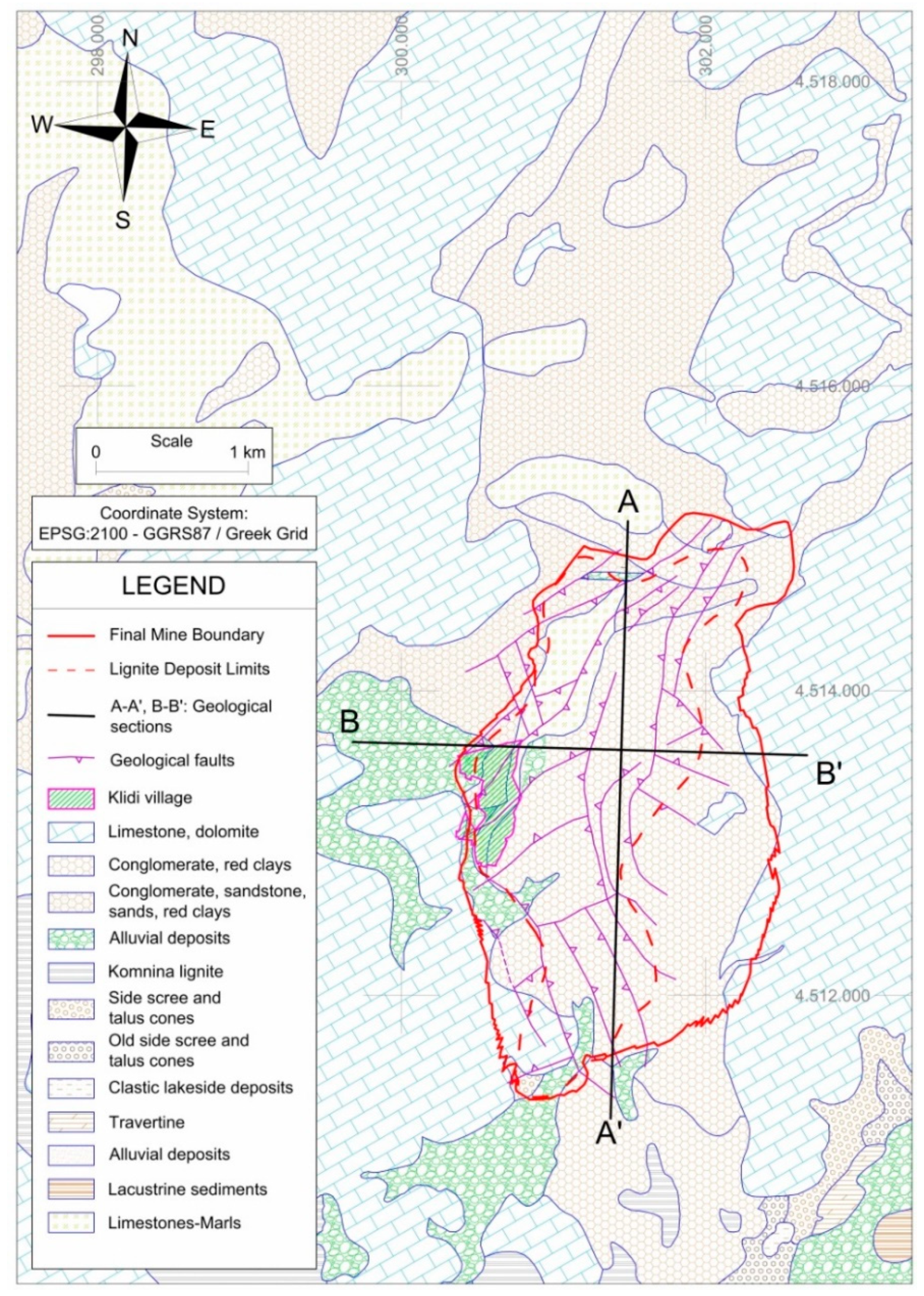
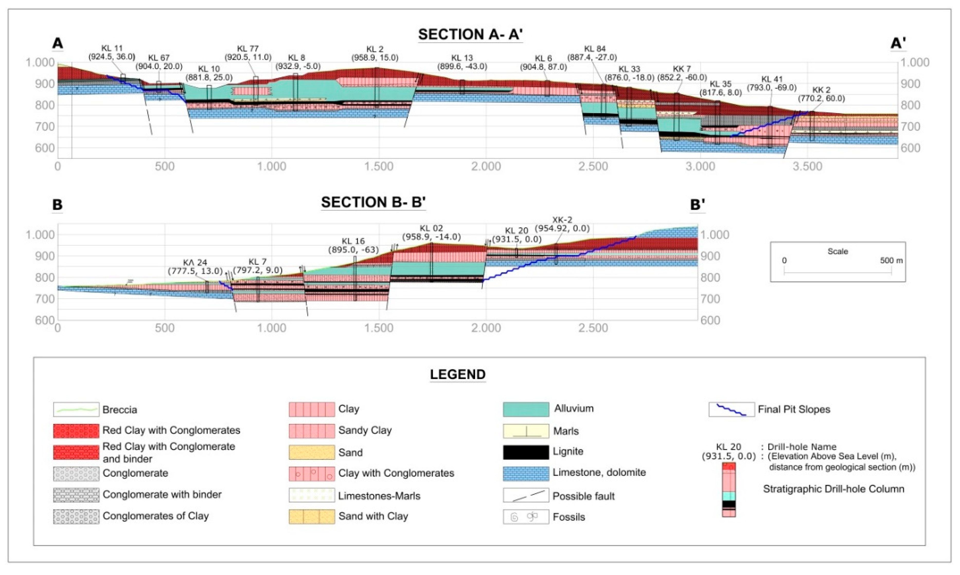
The deposit of the Klidi mine is divided into partly narrow blocks by several fault systems (Figure 3), which mainly strike in a NW–SE, NE–SW and N–S direction and mostly consist of normal and, to a lesser extent, of reverse faults with slight faulting in the underlying seams. The effect of these faults on the stratigraphy is shown in sections A-A´ and B-B´ (Figure 4).

The overlying strata thickness ranges from approximately 3 m up to 100 m. The layer series is composed of finely clastic, sandy clays and calcareous clayey marls with coarsely clastic, marly sands, sandy gravels and pebbles (Figure 4). Furthermore, overlying strata locally incorporate consolidated layers, the so-called Klidi formation, which may impede mining operations. This formation is distributed in high percentage over the mining area and predominantly consists of consolidated conglomerates with gravels and disk-shaped stones. The excavation of this formation may require blasting. The overall thickness of the lignite-bearing series (including intermediate seams) ranges between approximately 3 and 50 m [24,25].

3. Drilling Campaign

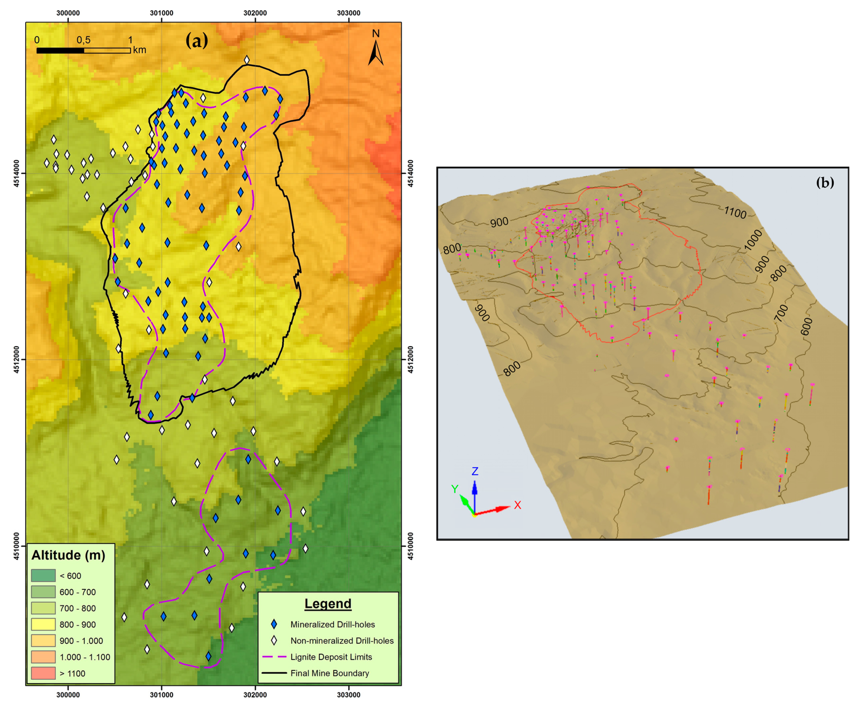
The drilling campaign for the Klidi lignite deposit includes 128 drill-holes, where 76 are mineralized, and was performed mainly during the period 1992–2011. The locations of the drill-holes and the mine surface limits are shown in Figure 5. The distance between the nearest drill-holes varies from 30 m to 500 m with an average of 200 m. The drill-hole density in the area of the Klidi surface mine is approximately 13 drill-holes per km².

The principal component analysis is based on the drilling survey data in the region of the Klidi lignite deposit in order to determine the principal components (axis or so-called factors). The primary core sample data refer to 128 vertical exploratory drill-holes in an area of 10 km². In these 128 drill-holes a total of 795 lignite seams and 1517 waste seams were recorded. The total thickness of the 795 lignite seams amounts to 689.0 m, while the total thickness of the 1517 waste seams amounts to 13023.8 m. The main chemical analysis data of the 795 lignite seams, involve moisture content, ash (dry) content and lower calorific value.

4. Data Analysis

4.1. Methodology

The proposed application of PCA for deposit modeling and evaluation of a multi-seam coal deposit is mainly based on the selection and comparative spatial analysis of suitable variables considering the coal deposit parameters (Figure 1).

The PCA statistical approach is based on data derived from the integration of the available drill-hole exploration results into geological and geomorhological information of the deposit. This integration of the exploratory data is the key to understanding the structure of the deposit and the spatial distribution of the main deposit parameters.

The first step of the experimental analysis is to determine the missing quality characteristic values in the coal seams of the drill-holes, using multiple linear regression analysis. This process is described by Pavlides et al. [26].

The next step is the evaluation of the available drill-hole data, by applying a suitable algorithm [4] and taking into consideration specific technical, economic and other criteria. The mineralized area is determined according to the drill-hole evaluation results. The main variables, which adequately describe the spatial characteristics of the deposit and are also essential for the deposit modeling, are then selected. The results of the statistical analysis, as well as the spatial distribution of the selected variables, are useful for the PCA and the deposit modeling.

The following step refers to the main part of the research work, the application of a PCA and the spatial interpolation and mapping of the results in a GIS environment, in order to make the evaluation of the deposit possible. The final step refers to the analysis and interpretation of the results.

4.2. Drill-Hole Analysis and Evaluation

The determination of mineable lignite seams and the corresponding run-off-mine lignite quality is a process of compositing seams into blocks of exploitable lignite [1]. In addition, the profitability of individual seams and consequently the estimated reserves of the lignite deposit are affected by the extraction cost and the market price of the run-off-mine lignite.

The aim of the drill-hole data evaluation was to estimate the recoverable lignite reserves with average ash content (dry basis) ≤50% and lower calorific value ≥1700 kcal/kg, according to the specifications of the Meliti Power Plant.

The parameters of the exploitable lignite block formations, in each drill-hole, were the following [1]:

(a)

The minimum thickness of waste layers that can be excavated by selective mining.

(b)

The minimum thickness of lignite blocks that can be excavated by selective mining.

(c)

The quality characteristics of waste layers included in the compositing blocks.

(d)

The quality characteristics of lignite layers included in the compositing blocks.

(e)

The thickness of dilution with waste (surface dilution) and the thickness of mining lignite loss at the top and bottom of each block.

(f)

The densities of lignite layers, of waste layers included in the blocks, and of the waste layer at the top, and bottom of the lignite blocks.

(g)

The cut-off limits of the quality of the run-of-mine lignite.

The applied algorithm, for compositing seams into blocks of exploitable lignite and intermediate waste material, can be summarized in the following steps [1]:

• Define all seams of each drill-hole as lignite or waste according to their quality characteristics (ash, moisture and calorific value).
• Formulate intermediate waste blocks by successive non-lignite seams.
• Determine selectively excavated waste blocks according to minimum thickness for selective mining.
• Determine exploitable lignite blocks between waste blocks according to specific quantitative and qualitative criteria.
• Create the evaluation report including all quantitative and qualitative data for the overburden, all lignite blocks and all intermediate waste blocks of each drill-hole.

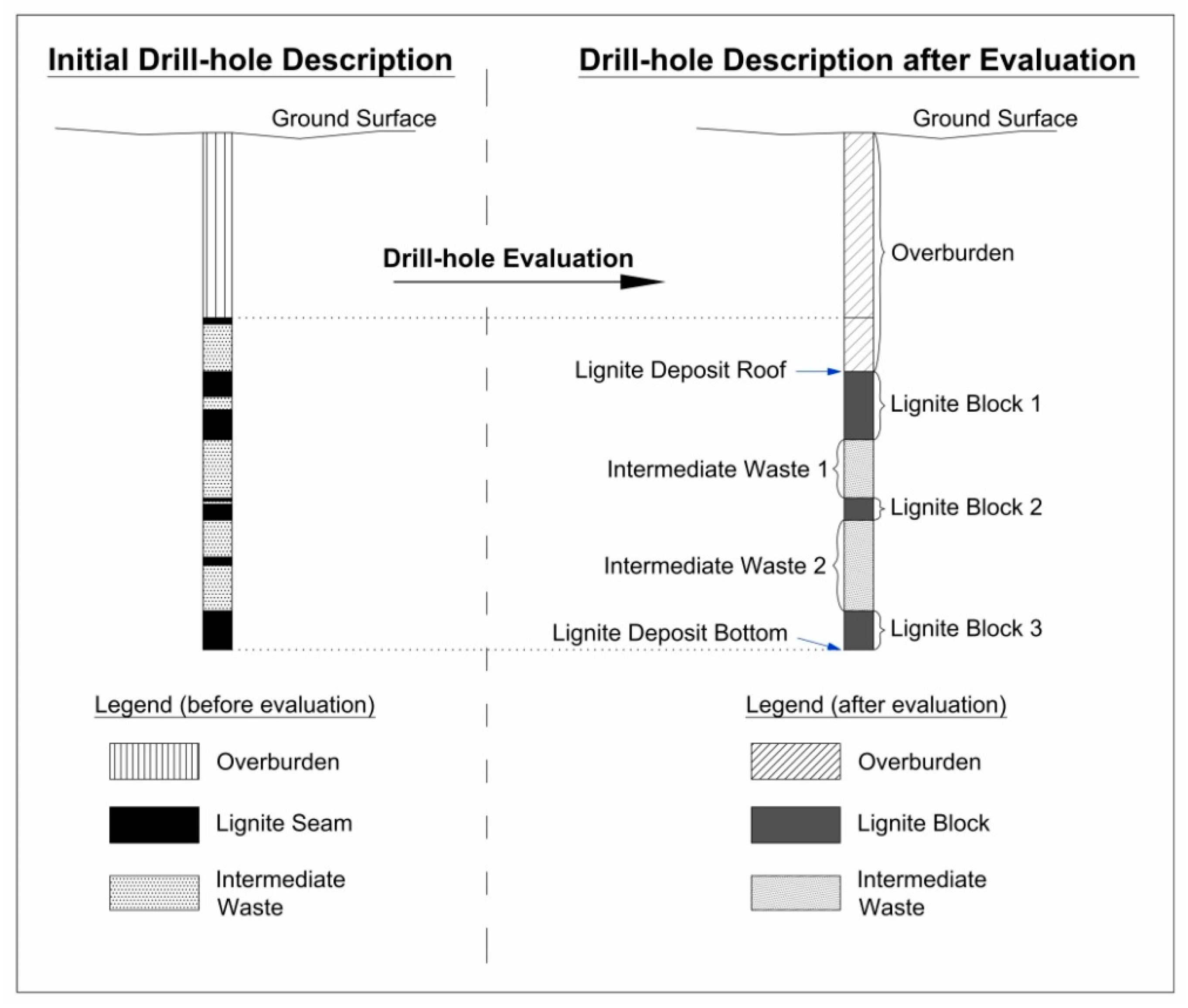
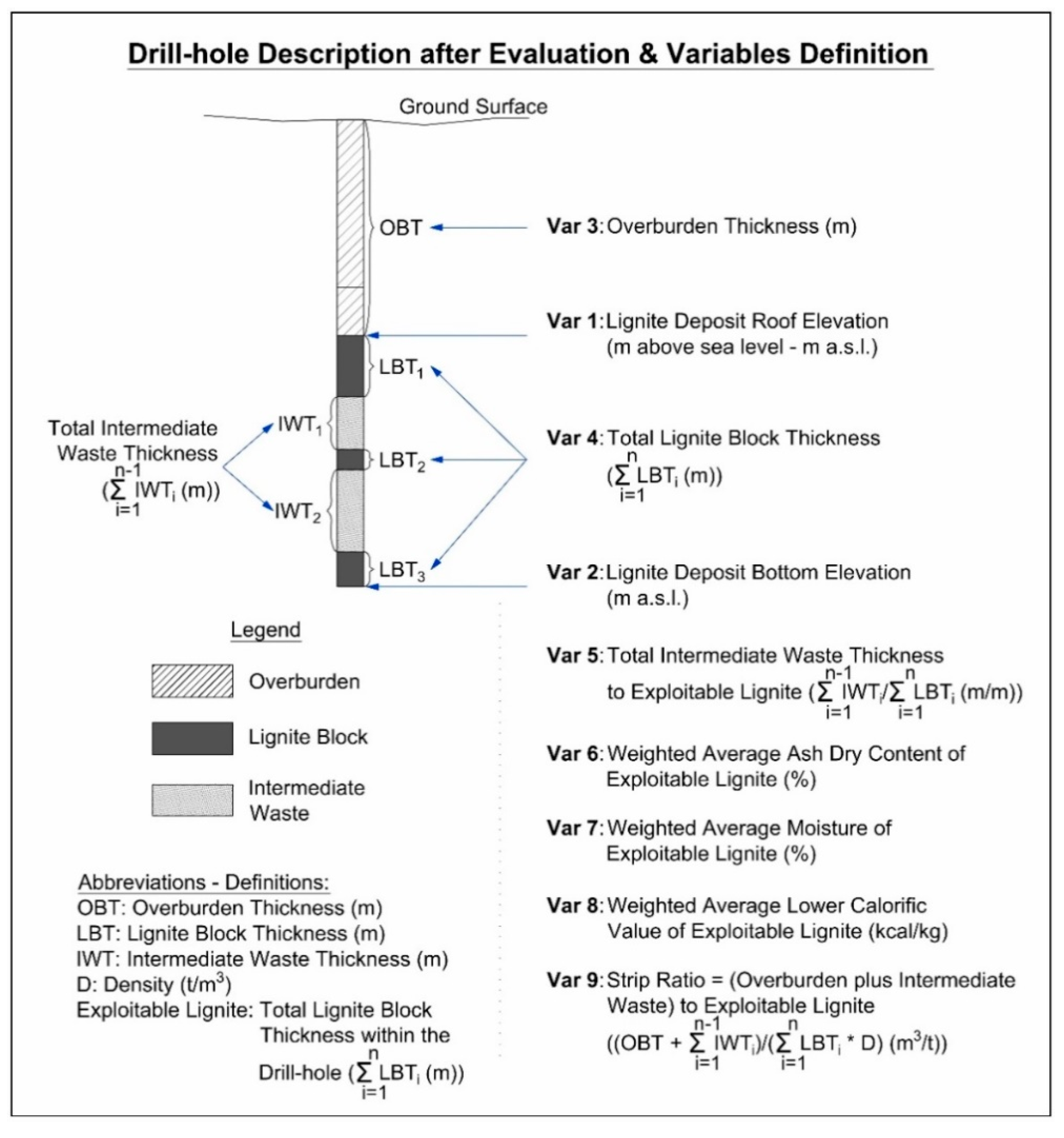
Figure 6 presents the initial drill-hole description and the drill-hole description after the evaluation algorithm. In this typical drill-hole evaluation example, the seven coal seams and the six intermediate waste seams of the initial drill-hole description, form three exploitable lignite blocks and two intermediate waste blocks respectively. Furthermore, the top of the higher lignite block defines the lignite deposit roof, the bottom of the lower lignite block defines the lignite deposit bottom and the material between the ground surface and the lignite deposit Roof and defines the overburden.

After applying drill-hole evaluation, with certain criteria in the above mentioned 128 drill-holes, 221 exploitable lignite blocks are formed, which have a total thickness of 645.4 m.

The nine variables that define the quantitative and qualitative characteristics of a multi-seam coal deposit and were selected for the application of a PCA are described and explained in Figure 7. These variables represent the main mineral deposit parameters that affect the exploitability of the deposit and should be considered in mine planning and design [27].

The statistical data and the spatial distribution of each variable were investigated to identify relationships with the geological structure of the deposit.

Table 1. Descriptive statistics of drill-hole variable values.

Variables Description		N	Range	Min	Max	Mean	Std. Deviation	Skewness	Kurtosis
Var 1	Lignite Deposit Roof Elevation (m a.s.l.)	76	519.94	428.02	947.96	773.63	114.59	−1.15	0.90
Var 2	Lignite Deposit Bottom Elevation (m a.s.l.)	76	520.09	426.96	947.05	750.06	118.89	−0.68	−0.08
Var 3	Overburden Thickness (m)	76	200.25	3.00	203.25	71.41	50.81	0.73	-0.43
Var 4	Total Lignite Block Thickness (m)	76	23.40	0.50	23.90	8.49	5.47	0.43	-0.26
Var 5	Total Intermediate Waste Thickness to Exploitable Lignite (m/m)	76	9.11	0	9.11	1.41	2.35	1.80	2.09
Var 6	Weighted Average Ash Dry Content of Exploitable Lignite (%)	76	48.26	18.32	66.58	36.63	10.69	0.57	−0.32
Var 7	Weighted Average Moisture of Exploitable Lignite (%)	76	20.35	30.24	50.59	43.87	3.54	−0.91	1.94
Var 8	Weighted Average Lower Calorific Value of Exploitable Lignite (kcal/kg)	76	1553.00	762.00	2315.00	1726.35	362.05	−0.46	−0.37
Var 9	Strip Ratio (m3/t)	76	150.64	0.83	151.47	14.84	25.44	3.73	15.08

includes the most important statistical data of all drill-holes, for the selected variables.

4.3. Principal Component Analysis

A PCA is an unsupervised explanatory analysis method for composite phenomena (factor analysis methods). In detail, it is a multi-dimensional statistical analysis method, which specializes in analyzing big data volumes. The PCA is based on the correlation of various variables that describe the studied phenomenon and thus it demands significant correlation among the initial selected variables. The main targets of the analysis are discussed below.

4.3.1. Decrease of Data Volume

A PCA allows the definition of limited number of new composite variables (components or factors) that ensures the simplification of a data set [28]. Each of the new components refers to a unique dimension of the studied phenomenon. Consequently, the new composite components are not correlated, in contrast with the initial variables. Data volume decrease is accomplished when the lowest possible modification of the distances among the observations is ensured.

4.3.2. Identification of Primary Variable Relationships (That Are Not Initially Obvious)

The new components produced by PCA scores are linear combinations of the initial variables. The first step of the method is the standardization of the data set (z-scores). The following basic step of a PCA, is setting up the covariance matrix of the data set. It must be noticed that the covariance is always measured between two dimensions (variables). If the covariance value is positive it indicates that both dimensions (variables) increase together. On the other hand, if the value is negative, then when one dimension increases the other decreases. A zero-covariance value indicates that the two variables are independent of each other.

In a multidimensional data set (more than two variables) the covariance matrix is created as follows (e.g., three variables X, Y, Z):

$$C=\left(\begin{array}{ccc}cov\left(X,X\right)& cov\left(X,Y\right)& cov\left(X,Z\right)\\ cov\left(Y,X\right)& cov\left(Y,Y\right)& cov\left(Y,Z\right)\\ cov\left(Z,X\right)& cov\left(Z,Y\right)& cov\left(Z,Z\right)\end{array}\right)$$

(1)

It can be noticed that along the main diagonal of the covariance matrix, the covariance value is between one dimension (variable) and itself, which means that these are the variances for that dimension. Moreover, since cov(a,b) = cov(b,a) the matrix is symmetrical about the main diagonal.

In the next phase of the analysis the eigenvectors and eigenvalues of the covariance matrix are calculated. For an m × m matrix there are m eigenvectors and all of them are perpendicular to each other, irrespective of how many dimensions (variables) there are. Eigenvalues and eigenvectors are calculated based on the following equations.

$$Cv=\lambda v$$

(2)

$$v=\left(\begin{array}{c}{a}_1\\ a_2\\ \begin{array}{c}⋮\\ a_m\end{array}\end{array}\right)$$

(3)

where,

• $C$ = covariance matrix
• $v$ = an eigenvector
• $\lambda$ = an eigenvalue
• $a_1$, $a_2$, …, $a_m$ = eigenvector values

Eigenvectors are the weights of the initial variables in the new dimensions of the phenomenon (principal components). For example, principal component 1 (PC₁) will have the following form:

$$P{C}_1=a_1{X}_1+a_2{X}_2+\cdots +a_m{X}_m$$

(4)

where,

• $a_1$, $a_2$, …, $a_m$ = eigenvector values for PC₁
• $X_1$, $X_2$, …, $X_m$ = initial variables

Consequently, after the calculation of all the eigenvectors of the covariance matrix

Table 2. Eigenvectors (Principal Components).

		Principal Components (Eigenvectors)
		PC1	PC2	…	PCm
Variables (dimensions)	Var 1	$a_1$	$b_1$	…	$k_1$
	Var 2	$a_2$	$b_2$	…	$k_2$
	…	…	…	…	…
	Var m	$a_m$	$b_m$	…	$k_m$

is produced:

Eigenvalues represent the total amount of variance that can be explained by a given principal component.

Table 3. Eigenvalues and total variance explained.

Principal Component	Eigenvalue	% of Variance	Cumulative %
PC1	${\lambda }_1$	${\pi }_1$	${\rho }_1$
PC2	${\lambda }_2$	${\pi }_2$	${\rho }_2$
…	…	…	…
PCm	${\lambda }_m$	${\pi }_m$	${\rho }_m$

, which is produced by the analysis process, illustrates that the first component explains the most variance, and the last component explains the least.

where,

• ${\lambda }_1$ > ${\lambda }_2$ > … > ${\lambda }_m$
• ${\pi }_1$ = ${\lambda }_1/m$, ${\pi }_2$ = ${\lambda }_2/m$, …, ${\pi }_m$ = ${\lambda }_m/m$
• ${\rho }_1$ = ${\pi }_1$, ${\rho }_2$ = ${\rho }_1$ + ${\pi }_2$, …, ${\rho }_m$ = ${\rho }_{m-1}$+ ${\pi }_m$

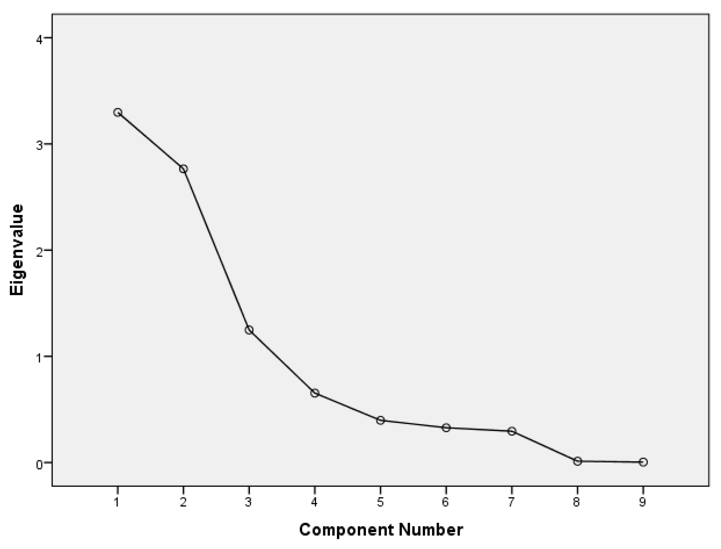
In order to choose the optimum number of principal components that best describes the phenomenon under study (thus decreasing the initial dimensions of the analysis) three criteria are used:

• The Guttman [29] and Kaiser [30] criterion, according to which only the principal components with eigenvalues greater than one are preserved. It should be mentioned that the reason for keeping components with eigenvalues greater than one is that these represent above average variance. The principal components with eigenvalues lower than one describe a low percentage of the initial data dispersion by each primary variable. Therefore, there is no point in keeping them.
• The Cattell [31] criterion, according to which only the principal components that are found above the line break in the scree plot are preserved.
• The selected number of principal components must explain a sufficient percentage of the total variance of the initial variables.

The next step of the analysis concerns the calculation of the component loadings. These values correspond to the correlation of each variable (dimension) with the principal component. Component loadings are calculated based on the following equation:

$$\begin{array}{l}{\mathrm{PC}}_1:\hspace{1em}\hspace{1em}c{l}_{1,n}=a_n\sqrt{{\lambda }_1}\\ {\mathrm{PC}}_2:\hspace{1em}\hspace{1em}c{l}_{2,n}=b_n\sqrt{{\lambda }_2}\\ \dots \hspace{1em}\hspace{1em}\hspace{1em}\dots \\ {\mathrm{PC}}_{\mathrm{m}}:\hspace{1em}\hspace{1em}c{l}_{m,n}=k_n\sqrt{{\lambda }_m}\end{array}$$

(5)

where,

• $c{l}_{m,n}$ = component loading for variable n for PC_m
• $a_n$, $b_n$, …, $k_n$ = PC value for variable n for PC₁, PC₂, …, PC_m correspondingly

$${\lambda }_m=\mathrm{eigenvalue}\mathrm{of}{\mathrm{PC}}_{\mathrm{m}}$$

$$n=1,2,\dots m$$

Table 4. Principal component loadings matrix.

		Principal Component
		PC1	PC2	…	PCm
Variables	Var 1	$c{l}_{1,1}$	$c{l}_{2,1}$	…	$c{l}_{m,1}$
	Var 2	$c{l}_{1,2}$	$c{l}_{2,2}$	…	$c{l}_{m,2}$
	…	…	…	…	…
	Var m	$c{l}_{1,n}$	$c{l}_{2,n}$	…	$c{l}_{m,n}$

is generated based on Equation (5). Each variable has a loading corresponding to each of the m components. For example, Var₁ is correlated cl_1,1 with PC₁, cl_2,1 with PC₂ and so on.

The basic principles of component loadings are:

• The square value of each loading represents the variance proportion, of the specific variable, explained by the corresponding component.

$${\left(c{l}_{m,1}\right)}^{2}100=p_{m,1}\%$$

(6)

The total variance, of the specific variable, is explained by the sum of all the square values of the component values. This is known as the communality.

$$p_{1,1}+p_{2,1}+\cdots +p_{m,1}=100\%$$

(7)

• The sum of the square values of all the component loadings for all the variables of a specific PC is the eigenvalue of this PC.

$${\left(c{l}_{m,1}\right)}^2+{\left(c{l}_{m,2}\right)}^2+\cdots +{\left(c{l}_{m,n}\right)}^2={\lambda }_m$$

(8)

The final step of the analysis is the estimation of the component scores. At first the component score coefficient matrix (

Table 5. Principal component (PC) score coefficient matrix.

		Principal Component
		PC1	PC2	…	PCm
Variables	Var 1	$c{s}_{1,1}$	$c{s}_{2,1}$	…	$c{s}_{m,1}$
	Var 2	$c{s}_{1,2}$	$c{s}_{2,2}$	…	$c{s}_{m,2}$
	…	…	…	…	…
	Var m	$c{s}_{1,n}$	$c{s}_{2,n}$	…	$c{s}_{m,n}$

) is calculated by dividing the component loadings by the eigenvalues according to Equation (9).

$$\begin{array}{l}{\mathrm{PC}}_1:\hspace{1em}\hspace{1em}c{s}_{1,n}=\frac{c{l}_{1,n}}{{\lambda }_1}\\ {\mathrm{PC}}_2:\hspace{1em}\hspace{1em}c{s}_{2,n}=\frac{c{l}_{2,n}}{{\lambda }_2}\\ \dots \hspace{1em}\hspace{1em}\hspace{1em}\dots \\ {\mathrm{PC}}_{\mathrm{m}}:\hspace{1em}\hspace{1em}c{s}_{m,n}=\frac{c{l}_{m,n}}{{\lambda }_m}\end{array}$$

(9)

where,

• $c{s}_{m,n}$ = component score coefficient for variable n for PC_m
• $c{l}_{m,n}$ = component loading for variable n for PC_m
• ${\lambda }_m$ = eigenvalue of PC_m
• $n$ = $1$, $2$, …, $m$

Consequently, $P{C}_{1,score}$ will be calculated by the following equation, and so on:

$$P{C}_{1,score}=c{s}_{1,1}+c{s}_{1,2}+\dots +c{s}_{1,n}$$

(10)

Evaluation of PCA results:

• For each component, at least two initial variables must present significant loadings: $\left|c{l}_{m,n}\right|>0.40$
• Each initial variable must contribute in at least a good level in one component.
• The “interpretation” of the principal components (based on the loadings) must be easy.

It must be underlined that, according to Comrey and Lee [32], the evaluation of the contribution of each initial variable in a principal component is:

• Excellent when $\left|c{l}_{m,n}\right|>0.71$
• Very good when $\left|c{l}_{m,n}\right|>0.63$
• Good when $\left|c{l}_{m,n}\right|>0.55$
• Moderate when $\left|c{l}_{m,n}\right|>0.45$

The application of a PCA in this work is based on the evaluated drill-hole data of a multi-seam lignite deposit as described in Section 4.2. The geometric basic elements of the lignite deposit and other deposit quantitative and qualitative parameters records were considered as parameters (explanatory variables). Each one of the selected principal components that were calculated corresponds to a group of parameters that contribute strongly to the total variance of data cloud [33].

5. Results

5.1. Principal Components

Principal Components (eigenvectors) and eigenvalues were calculated by applying equations one through three on the variable values of the drill-hole dataset, thus constructing the corresponding theoretical Table 2 and Table 3.

Table 6. Principal components (eigenvectors).

	Principal Component
	1	2	3	4	5	6	7	8	9
Var 1	0.4456	−0.2998	0.0407	−0.0715	0.3490	−0.0632	0.3663	0.1516	−0.6494
Var 2	0.4212	−0.3400	−0.1599	−0.0900	0.3226	−0.0896	0.2002	−0.1473	0.7067
Var 3	−0.2135	0.4275	−0.2084	0.1313	0.8183	0.1618	−0.1215	−0.0108	−0.0184
Var 4	0.2728	0.3760	0.3521	−0.0600	−0.1076	0.7027	0.3694	−0.0159	0.1206
Var 5	−0.1276	0.1127	0.7995	0.1612	0.2038	−0.4708	0.1560	−0.0561	0.1231
Var 6	−0.3297	−0.4470	0.1835	0.0432	0.1325	0.3102	−0.0454	0.7151	0.1693
Var 7	0.3702	0.1048	−0.0998	0.8706	−0.1236	−0.0475	−0.0934	0.2364	0.0442
Var 8	0.2128	0.4960	−0.1505	−0.3658	−0.0867	−0.3694	0.0841	0.6200	0.1294
Var 9	−0.4435	0.0267	−0.3160	0.2153	−0.1048	−0.1065	0.7952	−0.0130	0.0394

, which is the equivalent of Table 2, presents each eigenvector (principal component) expressed by its relation with each one of the nine variables according to Equation (4).

Table 7. Eigenvalues and % of explained variance.

Principal Component	Eigenvalues
	Total	% of Variance	Cumulative %
1	3.297	36.636	36.636
2	2.765	30.723	67.360
3	1.248	13.868	81.228
4	0.654	7.261	88.489
5	0.397	4.413	92.902
6	0.328	3.641	96.542
7	0.295	3.275	99.817
8	0.012	0.139	99.956
9	0.004	0.044	100

, which is the equivalent of Table 3, presents the calculated eigenvalue for each eigenvector along with the percentage of variance explained by it. As mentioned above, and shown in Table 7, the cumulative variance explained by the first three eigenvectors is about 81%. Based on the three criteria mentioned in Section 4.3, which briefly are (a) eigenvalue greater than 1, (b) scree plot line break (Figure 8) and (c) cumulative variance explained, the first three principal components where preserved for the analysis, while the rest were discarded.

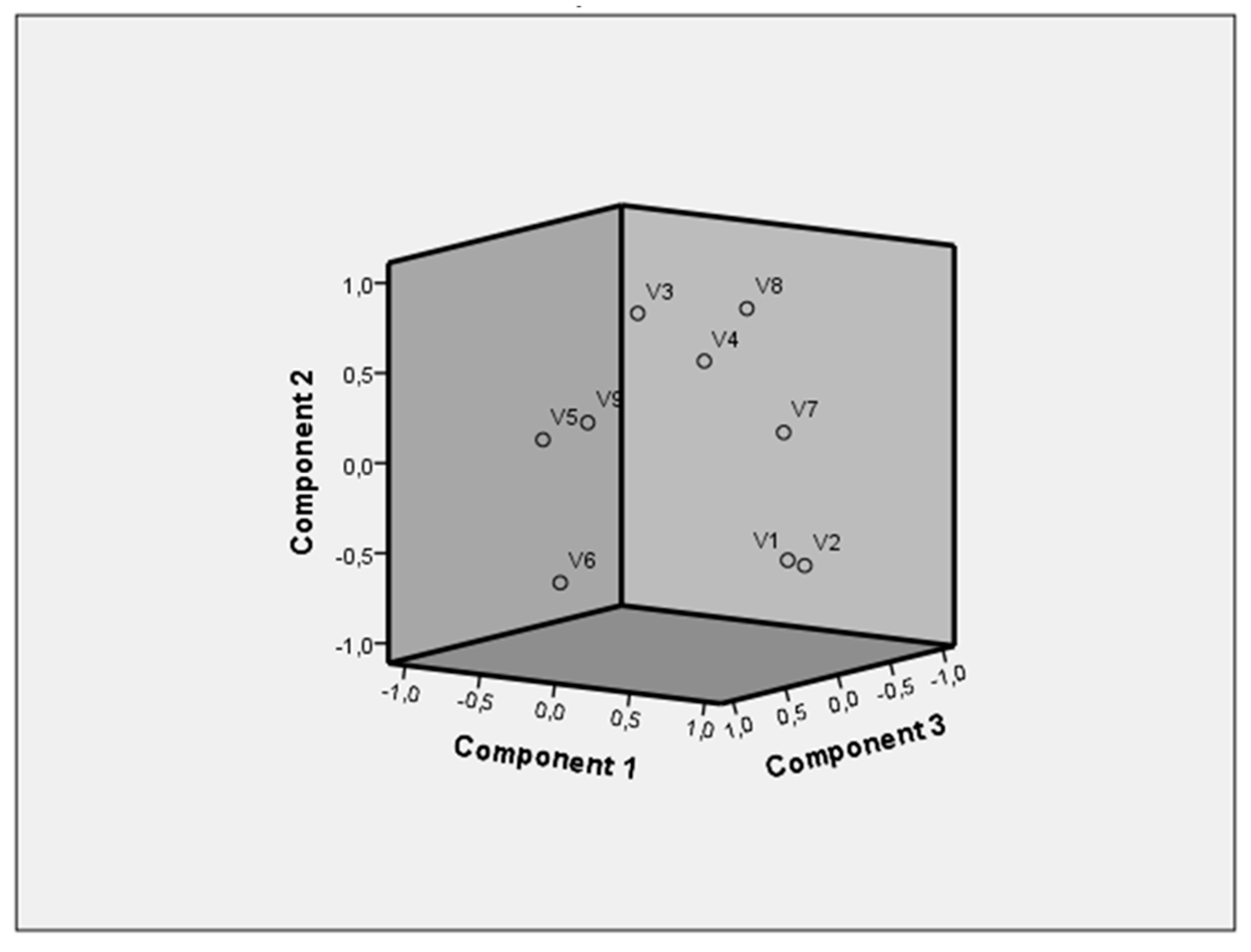
The correlation of each variable with each principal component (component loadings) is calculated via Equation (7) and presented in

Table 8. Matrix of Principal Component Loadings.

	Principal Component
	1	2	3	4	5	6	7	8	9
Var 1	0.809	−0.499	0.045	−0.058	0.220	−0.036	0.199	0.017	−0.041
Var 2	0.765	−0.565	−0.179	−0.073	0.203	−0.051	0.109	−0.016	0.045
Var 3	−0.388	0.711	−0.233	0.106	0.516	0.093	−0.066	−0.001	−0.001
Var 4	0.495	0.625	0.393	−0.048	−0.068	0.402	0.201	−0.002	0.008
Var 5	−0.232	0.187	0.893	0.130	0.128	−0.269	0.085	−0.006	0.008
Var 6	−0.599	−0.743	0.205	0.035	0.084	0.178	−0.025	0.080	0.011
Var 7	0.672	0.174	−0.111	0.704	−0.078	−0.027	−0.051	0.026	0.003
Var 8	0.386	0.825	−0.168	−0.296	−0.055	−0.211	0.046	0.069	0.008
Var 9	−0.805	0.044	−0.353	0.174	−0.066	−0.061	0.432	−0.001	0.002

, which is the equivalent of the theoretical Table 4. Figure 9 presents the position of each variable (loadings) in the 3D space created by the three selected principal components. As can be deduced from Table 8 and Figure 9, groups of variables are created depending on the level and nature of their correlation with the components. For example, Var 1 (V1) and Var 2 (V2) are highly and positively correlated with PC1, Var 3 (V3), Var 4 (V4) and Var 8 (V8) are highly and positively correlated with PC2, Var 5 (V5), Var 6 (V6) and Var 9 (V9) are negatively correlated with PC1, and so on. This grouping can help to explain the natural sense of the interrelationship of the grouped variables, as well as the general concept described by the component that groups them.

Finally, in order to spatially plot and evaluate the PCs, component scores are calculated. At first the component score coefficient matrix is created (

Table 9. Principal Component Score Coefficient Matrix.

	Principal Component
	1	2	3	4	5	6	7	8	9
Var 1	0.245	−0.180	0.036	−0.088	0.554	−0.110	0.675	1.358	−10.299
Var 2	0.232	−0.204	−0.143	−0.111	0.512	−0.157	0.369	−1.319	11.207
Var 3	−0.118	0.257	−0.186	0.162	1.298	0.283	−0.224	−0.097	−0.292
Var 4	0.150	0.226	0.315	−0.074	−0.171	1.228	0.680	−0.143	1.913
Var 5	−0.070	0.068	0.716	0.199	0.323	−0.822	0.287	−0.502	1.952
Var 6	−0.182	−0.269	0.164	0.053	0.210	0.542	−0.084	6.404	2.684
Var 7	0.204	0.063	−0.089	1.077	−0.196	−0.083	−0.172	2.117	0.701
Var 8	0.117	0.298	−0.135	−0.452	−0.138	−0.645	0.155	5.552	2.052
Var 9	−0.244	0.016	−0.283	0.266	−0.166	−0.186	1.465	−0.116	0.625

), which is the equivalent of the theoretical Table 5 by applying Equation (9) and then the scores are calculated using Equation (10).

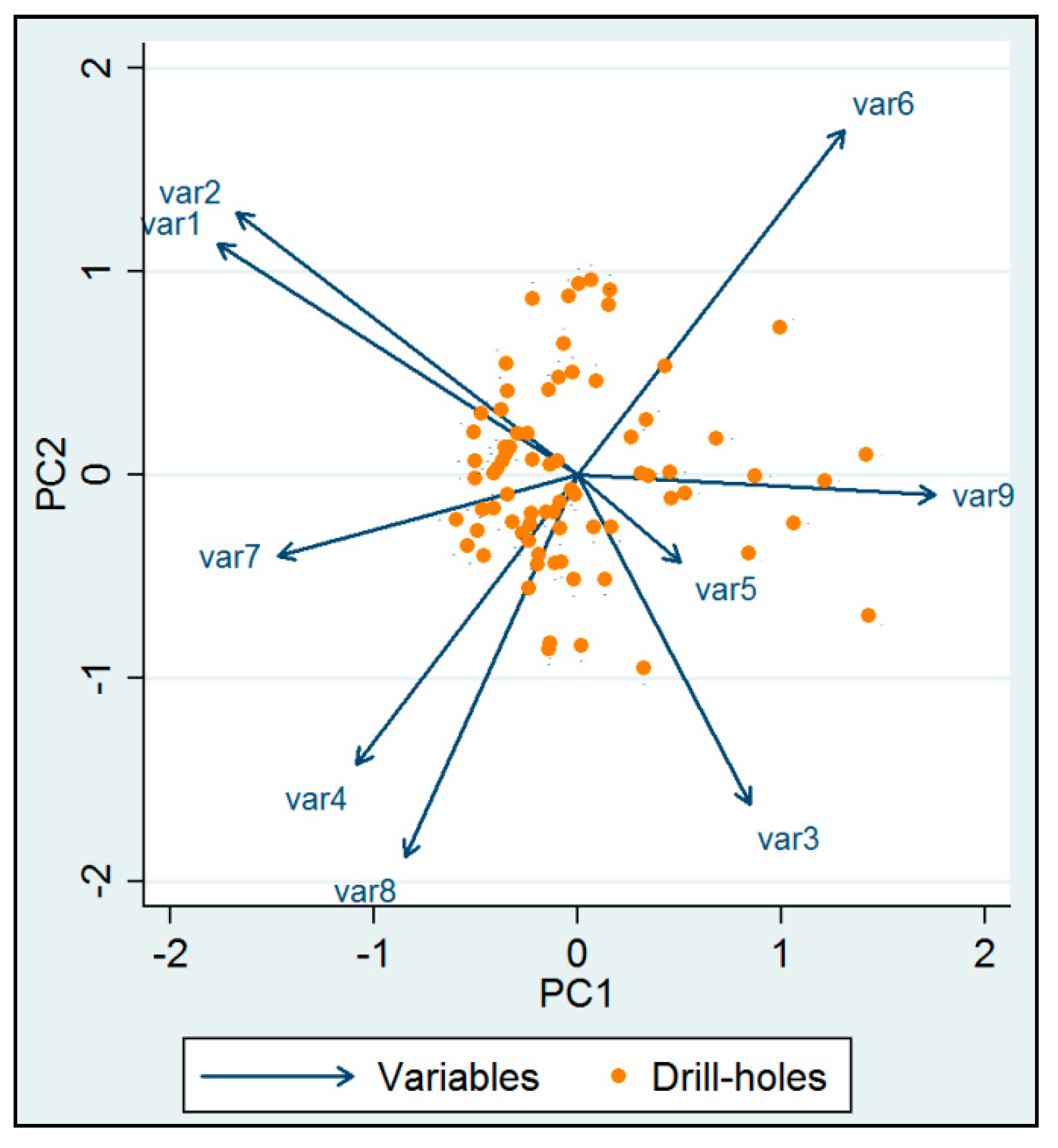
The biplot in Figure 10 presents (a) the position of the drill-holes according to the scores (coordinates) that each one of them acquired in the first two principal components, along with (b) the component loading vectors of the variables. This plot makes it easier to compare and group the drill-holes. Those with similar profiles in the biplot will cluster together. For example, a group of drill-holes can be identified in the area around the Var 4 vector and another one between the Var 2 and Var 6 vectors. This is an extremely useful output of the biplot as it leads to the interpretation of the characteristics that either have similar effect to the drill-holes and thus group them or have an opposite effect in them and thus differentiate them. In brief, this output feature of the biplot helps to identify the interrelationships of the drill-holes within groups, as well as the differences among groups.

In parallel, the component loading vectors interpret the level of influence that each variable has in each of the two main PCs, as well as the way that they correlate with one another. As can be seen in the biplot all variable vectors are pinned at the origin of PCs, meaning the point where both axes intersect (PC1 = 0, PC2 = 0). The further away a vector is from a PC origin (projection length in each axis) the more influence it has on that PC. Furthermore, when two vectors have a small angle between them (e.g., Var 1 and Var 2) the variables they represent are positively correlated. When two vectors form a large angle between them (close to 180°) the variables they represent are negatively correlated (e.g., Var 4 and Var 6). Finally, when the angle between two vectors is about 90° then the corresponding variables are not correlated (e.g., Var 2 and Var 6).

Taking into account that each one of the three principal components that were identified corresponds to a group of parameters that contribute strongly to the total variance of the data cloud, they are important for interpreting the geological characteristics of the mine site.

5.2. Spatial Analysis

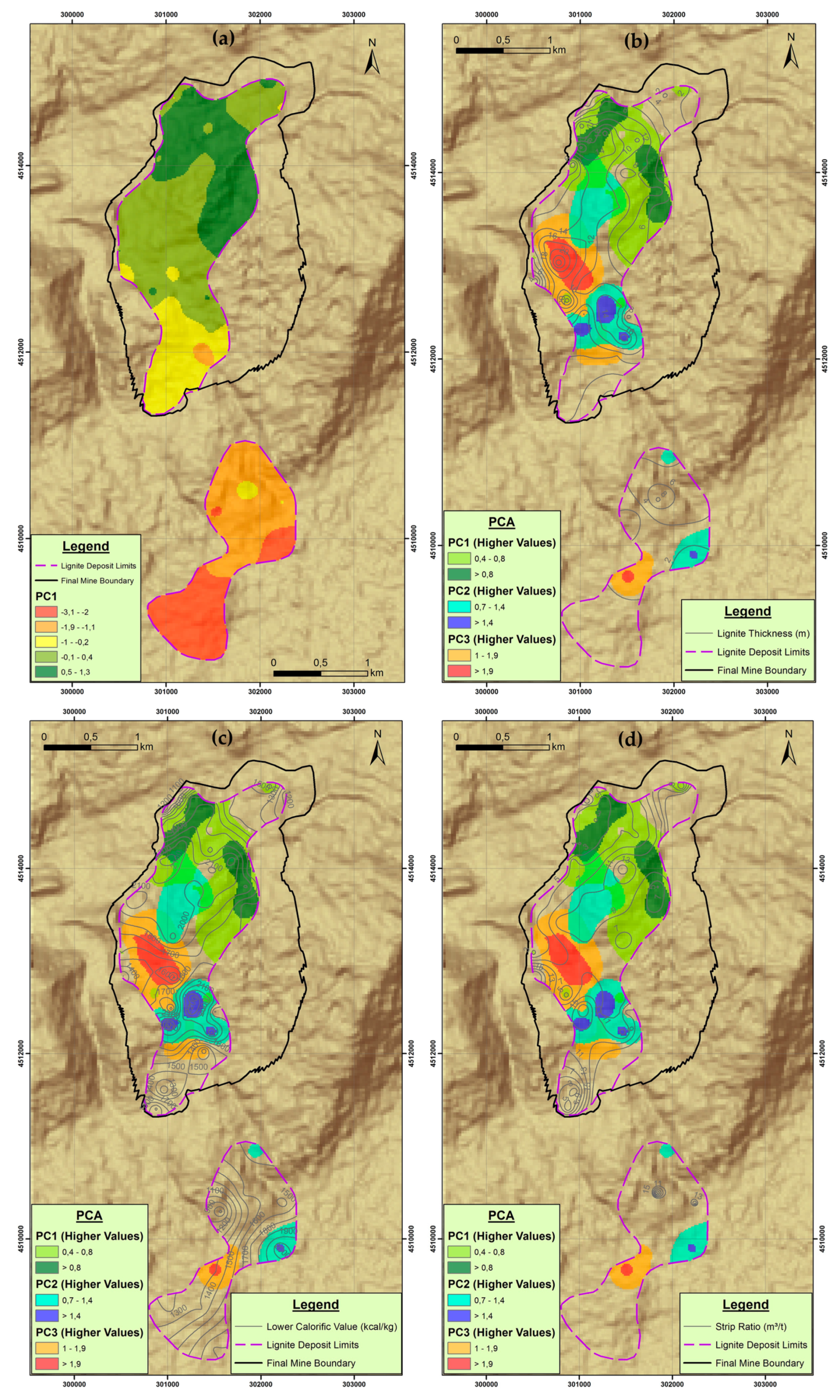
Spatial analysis was carried out through GIS techniques. PC scores were interpolated with the Kriging method and spatially delimited (masked) by the lignite deposit limits. These PC values were spatially rasterized by the drill-hole points. The produced PC raster layers were then reclassified after many trials, where various data classification methods were tested (natural breaks, geometrical interval, defined interval, etc.). Finally, the classification method that best presented the higher PC values was selected for the raster layers. In parallel, the spatial distribution contours of the three characteristic variables (lignite thickness, lower calorific value, strip ratio) were calculated. Furthermore, for clearer understanding of the area’s morphology the Hillshade raster layer [34] was produced by the digital elevation model (DEM), which was acquired by the database of the Advanced Spaceborne Thermal Emission & Reflection Radiometer Global Digital Elevation Model (ASTER GDEM) satellite project [35]. DEM and Hillshade were limited (masked) to a slightly wider area from the lignite deposit limits and were used as background layers. Finally, in order to sufficiently map the results of the previous analysis, the cartographic overlay (CO) technique was implemented as shown in Figure 11 and Figure 12. All spatial analysis and mapping steps took place in a GIS environment.

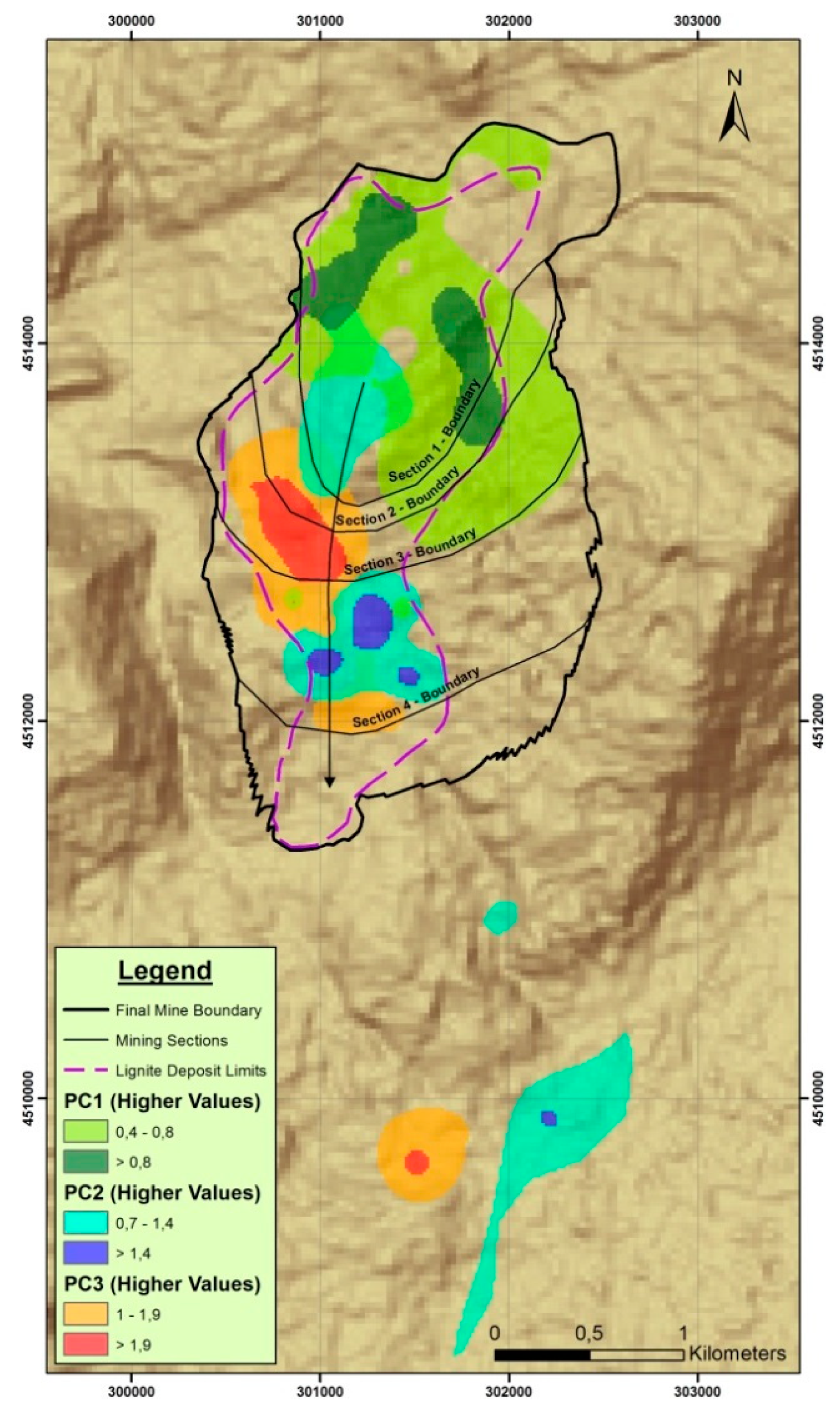
As mentioned above, three basic principal components were identified, PC1, PC2 and PC3, corresponding altogether to 81% of the total cloud variance. The comparative spatial interpolation of PC1, PC2 and PC3 higher values in combination with the spatial distribution of the characteristic variables lignite thickness (Var 4), lower calorific value (Var 8) and strip ratio (Var 9) are shown in Figure 11. The spatial distribution of PC1, PC2 and PC3 higher values in relation to strategic mine planning and the sectors of mine development and mine extraction sequencing are shown in Figure 12.

6. Discussion

From Figure 10 it can be deduced, as far as the variables of the Klidi deposit are concerned, that the strong positive correlation between lignite deposit roof elevation (Var 1) and lignite deposit bottom elevation (Var 2) is associated with the formation of the lignite deposit and the lignite-bearing sequence in relation to the sedimentation in the basin. A positive correlation also exists between the total lignite block thickness (Var 4) and the weighted average lower calorific value of exploitable lignite (Var 8), indicating the coexistence of these two main parameters that contribute to the exploitability of the deposit. In contrast, the weighted average lower calorific value of exploitable lignite (Var 8) and the weighted average ash dry content of exploitable lignite (Var 6) are negatively correlated indicating low fluctuations of moisture content within the deposit. In this context, a low total intermediate waste thickness to exploitable lignite (Var 5) is negatively correlated with the lignite deposit roof elevation (Var 1) and the lignite deposit bottom elevation (Var 2). Furthermore, the lignite deposit bottom elevation (Var 2) and the weighted average ash dry content of exploitable lignite (Var 6) are not correlated. This result is related to the structure of the deposit. A similar result is also obtained for the lignite deposit bottom elevation (Var 2) and the total lignite block thickness (Var 4). In conclusion, the initially expected correlations among the variables are confirmed by the biplot, a fact that verifies the accuracy of the primary data and the effective application of a PCA.

PC1 higher values are dominant in the mineralized area, which is located in the northeast part of the deposit (Figure 11). This area is defined by the NE–SW oriented major faults. The higher values of PC1 are positively related to high elevation of the lignite deposit roof (Var 1), high elevation of the lignite deposit bottom (Var 2), high total lignite block thickness (Var 4) and high moisture content of exploitable lignite (Var 7) in combination with high lower calorific value (Var 8). The negative values of PC1 in the component score coefficient matrix (Table 9) are related to low overburden thickness (Var 3), low total intermediate waste thickness to exploitable lignite (Var 5), low ash dry content of exploitable lignite (Var 6) and low strip ratio (Var 9). All these characteristics correspond to favorable conditions that increase the deposit exploitability. Therefore, this area is suitable for the location of the box cut and the initial opening phase of the mine (Sector 1 in Figure 12). Considering the mine investment analysis, this area is characterized by lower mining operating cost, increased annual lignite production, earlier start of lignite production, as well as better quality of the orebody comparing with the rest part of the lignite deposit.

The second component PC2 involves increased overburden thickness (Var 3), the total lignite block thickness (Var 4) and the total intermediate waste thickness to exploitable lignite (Var 5) in combination with increased lower calorific value (Var 8), corresponding to a less financially efficient mineralized area. PC2 higher values are dominant in the drill-holes which are mainly located in the eastern part of the deposit, next to mountain Voras and in the southeast part of the deposit next to Petron Lake.

The third component PC3 is positively related to high total lignite block thickness (Var 4), high total intermediate waste thickness to exploitable lignite (Var 5), high ash dry content of exploitable lignite (Var 6), low lignite deposit bottom elevation (Var 2), the overburden thickness (Var 3), the low calorific value (Var 8), as well as low strip ratio (Var 9). PC3 higher values are dominant mainly in the central part of the deposit and characterize a low financially efficient mineralized area. The remaining principal components are considered insignificant, since each explains less than 8% of the total sampling cloud variance.

Based on the above results of PCA, the revealed spatial relationships of PC1, PC2 and PC3 permit a better understanding of the deposit structure regarding the spatial variability of the geometrical characteristics of the deposit, as well as of the lignite quality parameters. Furthermore, they are related to the mineralization pattern of the deposit (lignite deposit limits in Figure 11 and Figure 12) in combination with the orientation of the major faults (Figure 3 and Figure 4). The results also indicate that PCA can be a useful tool for orebody modeling and evaluation of multi-seam coal deposits.

In this framework, the results also highlighted that PCA can be used to efficiently analyze the spatial variability of specific deposit parameters that affect the cash flows of the mining project, estimate uncertainties, and optimize mine exploitation. In this way, the method can add value to mine planning. Taking into account that the design and scheduling phase in mine-planning is a multi-criteria, region and application-specific process, a scenario approach for the selection of the operation mode (direction of mine development and a parallel or a slewing pattern or a combination of both) could be based on the spatial distribution of the three principal components that were identified.

Considering the PCA results in relation to mine planning and design of the Klidi mine, the final mine boundary as well as the strategic mine development according to the successive excavation Sectors 1–4 (Figure 12) is completely justified. The separated mineralized zone in the south is not significant according to the results of drill-holes evaluation. Considering the mine boundary according to the mine design shown in Figure 12 the exploitable lignite reserves of the Klidi mine amount to 42 million tons with an average Strip Ratio of 10 m³ of waste per ton of lignite and an average lower calorific value of 1750 kcal/kg.

This sequence of mine exploitation phases is mainly related to the following two objectives regarding the geologic model of the mineral deposit:

(a)

Optimization of the mine operation and the lignite production schedule in relation to the time and spatial evolution of the strip ratio, based on discounted cash flow analysis, and

(b)

Minimization of waste outside dumping volume

Compared to previously published results which also employed a PCA process, the results obtained in the present work refer to the application of a PCA for exploratory data analysis of multi-seam deposits and revealed the contribution of a PCA to a quantitative understanding and an efficient analysis of the spatial variations regarding critical parameters for mine planning purposes.

For an integrated approach, the mineral deposit model is combined with suitable geotechnical and hydrogeological analysis, as well as with an environmental impact assessment and the corresponding financial analysis [36].

From the above analysis, it is obvious that a PCA can provide useful results considering the structural analysis of multi-seam coal deposits. Furthermore, it can be used to increase the efficiency of mine planning and design.

7. Conclusions

The implementation of principal component analysis on evaluated drill-hole data and its synergetic use with GIS spatial modeling techniques can become a very useful tool for mine planning and deposit structure identification. This integrated methodology can set the required criteria for optimum deposit segmentation, in terms of exploitation sequence, based on financial and other mining efficient parameters. This argument was proven in the present study, where the applied methodology in the Klidi area lignite deposit resulted in a productively suitable segmentation that was used for the exploitation planning and the progress of the mining works.

The revealed spatial relationships of the three principal components that were identified permit a better understanding of the deposit structure regarding the spatial variability of the geometrical characteristics of the deposit, as well as of the lignite quality parameters. Furthermore, they are related to the mineralization pattern of the deposit in combination with the orientation of the major faults. Therefore, the results are important for interpreting the geological characteristics of the mine site.

As a technique, a PCA can describe the variability of primary data and interpret their fluctuations and interrelationships, leading thus to the decrease of the initial dimensions of the studied phenomenon, in a way that no significant information is lost and at the same time the best understanding of the researched subject is deduced. This ability of this method along with GIS spatial analysis techniques, as was highlighted in the results of this study, is a well-suited approach for multi-seam deposit analysis, especially when big datasets (e.g., numerous records of drill-hole data) need to be processed, analyzed and evaluated. In parallel, in a more research perspective, this proposed methodology offers an alternative approach that can address the lack of analysis techniques when multi-seam deposits are concerned.

Compared with more traditional methods for the visualization of subsurface geology in multi-seam deposits based on drill-hole sequences and the data interpretation, a PCA can provide a deeper understanding of the related geological spatial variables. The principal advantage of the method lies in its ability to identify the dominant patterns among the variables and the deposit structure, contributing to the optimum planning of mine development.

References

1. Roumpos, C.P.; Paraskevis, N.I.; Galetakis, M.J.; Michalakopoulos, T.N. Mineable lignite reserves estimation in continuous surface mining. In Proceedings of the 12th International Symposium Continuous Surface Mining-Aachen 2014, Aachen, Germany, 21−23 September 2014. [Google Scholar]
2. Pavlides, A.; Hristopoulos, D.T.; Roumpos, C.; Agioutantis, Z. Spatial modeling of lignite energy reserves for exploitation planning and quality control. Energy 2015, 93, 1906–1917. [Google Scholar] [CrossRef]
3. Roumpos, C.; Pavloudakis, F.; Galetakis, M. Optimal production rate model for a surface lignite mine. In Proceedings of the 3rd AMIREG International Conference: Assessing the Footprint of Resource Utilization and Hazardous Waste Management, Athens, Greece, 7 February 2009. [Google Scholar]
4. Roumpos, C.; Partsinevelos, P.; Agioutantis, Z.; Makantasis, K.; Vlachou, A. The optimal location of the distribution point of the belt conveyor system in continuous surface mining operations. Simul. Mod. Pract. Theory 2014, 47, 19–27. [Google Scholar] [CrossRef]
5. Jolliffe, I.T.; Cadima, J. Principal Component Analysis: A review and recent developments. Philos. Trans. A Math. Phys. Eng. Sci. 2016, 374, 20150202. [Google Scholar] [CrossRef] [PubMed]
6. Roumpos, C.; Akylas, N.; Terezopoulos, N. A decision making model for lignite deposits exploitability. In Proceedings of the 13th International Symposium Mine Planning and Equipment Selection, Wrocław, Bolan, 1–3 September 2004. [Google Scholar]
7. Paraskevis, N.; Roumpos, C.; Stathopoulos, N.; Adam, A. Spatial analysis and evaluation of a coal deposit by coupling AHP & GIS techniques. Int. J. Min. Sci. Technol. 2019, (in press). [Google Scholar]
8. Lishchuk, V.; Lund, C.; Lamberg, P.; Miroshnikova, E. Simulation of a mining value chain with a synthetic ore body model: Iron ore example. Minerals 2018, 8, 536. [Google Scholar] [CrossRef]
9. Carvalho, J.P.; Dimitrakopoulos, R. Effects of High-Order Simulations on the Simultaneous Stochastic Optimization of Mining Complexes. Minerals 2019, 9, 210. [Google Scholar] [CrossRef]
10. Bhuiyan, M.; Esmaieli, K.; Ordóñez-Calderón, J.C. Application of Data Analytics Techniques to Establish Geometallurgical Relationships to Bond Work Index at the Paracutu Mine, Minas Gerais, Brazil. Minerals 2019, 9, 302. [Google Scholar] [CrossRef]
11. Barnett, R.M. Principal Component Analysis. In Geostatistics Lessons; Deutsch, J.L.; 2017; Available online: http://www.geostatisticslessons.com/lessons/principalcomponentanalysis.html (accessed on 3 May 2019).
12. Louloudis, G. The worth of hydro geochemical data factor analysis (PCA) in interpretation of underground water origin. Megalopolis lignite bearing fields mine water and regional waters relations case study. In Proceedings of the 15th International Conference on Environmental Science and Technology, Rhodes, Greece, 31 August–2 September 2017. [Google Scholar]
13. Ting-Nien, W.; Chiu-Sheng, S. Application of Principal Component Analysis and Clustering to Spatial Allocation of Groundwater Contamination. In Proceedings of the 5th International Conference on Fuzzy systems and Knowledge Discovery, Shandong, China, 18–20 October 2008; IEEE: Piscataway, NJ, USA, 2008; pp. 236–240. [Google Scholar]
14. Sideri, D. Ground subsidence’s investigation under Thessaly plain aquifers overexploited, based on geotechnical of formations behavior and geostatistical model results. Ph.D. Thesis, National Technical University of Athens, Athens, Greece, 2016. [Google Scholar]
15. Tesch, S.; Otto, M. Application of principal-component analysis to the interpretation of brown coal properties. Fuel 1995, 74, 978–982. [Google Scholar] [CrossRef]
16. Pandey, B.; Agrawal, M.; Singh, S. Assessment of air pollution around coal mining area: Emphasizing on spatial distributions, seasonal variations and heavy metals, using cluster and principal component analysis. Atmos. Pollut. Res. 2014, 5, 79–86. [Google Scholar] [CrossRef] [Green Version]
17. Ma, L.; Yang, Z.; Li, L.; Wang, L. Source identification and risk assessment of heavy metal contaminations in urban soils of Changsha, a mine-impacted city in Southern China. Environ. Sci. Pollut. Res. 2016, 23, 17058–17066. [Google Scholar] [CrossRef] [PubMed]
18. Ma, L.; Qian, J.; Zhao, W.; Curtis, Z.; Zhang, R. Hydrogeochemical analysis of multiple aquifers in a coal mine based on nonlinear PCA and GIS. Environ. Earth Sci. 2016, 75, 716. [Google Scholar] [CrossRef]
19. Liu, P.; Hoth, N.; Drebenstedt, C.; Sun, Y.; Xu, Z. Hydro-geochemical paths of multi-layer groundwater system in coal mining regions—Using multivariate statistics and geochemical modeling approaches. Sci. Total Environ. 2017, 601, 1–14. [Google Scholar] [CrossRef] [PubMed]
20. Atanacković, N.; Dragišić, V.; Stojković, J.; Papić, P.; Živanović, V. Hydrochemical characteristics of mine waters from abandoned mining sites in Serbia and their impact on surface water quality. Environ. Sci. Pollut. Res. 2013, 20, 7615–7626. [Google Scholar] [CrossRef] [PubMed]
21. Vallejuelo, S.F.O.; Gredilla, A.; Boit, K.; Teixeira, E.C.; Sampaio, C.H.; Madariaga, J.M.; Silva, L.F. Nanominerals and potentially hazardous elements from coal cleaning rejects of abandoned mines: Environmental impact and risk assessment. Chemosphere 2017, 169, 725–733. [Google Scholar] [CrossRef] [PubMed]
22. Dowd, P.A.; Xu, C.; Coward, S. Strategic mine planning and design: Some challenges and strategies for addressing them. Min. Technol. 2016, 125, 22–34. [Google Scholar] [CrossRef]
23. Roumpos, C.; Pavloudakis, F.; Liakoura, A.; Nalmpanti, D.; Arampatzis, K. Utilisation of lignite resources within the context of a changing electricity generation mix. In Proceedings of the 10th International Brown Coal Mining Congress, Bełchatów, Poland, 16–18 April 2018. [Google Scholar]
24. Roumpos, C.; Chatzisavas, K. Technical mining study of Klidi mine. Public Power Corporation of Greece. 2018; Unpublished study. (In Greek) [Google Scholar]
25. Kotis, T.; Ploumidis, M.; Metaxas, A.; Varvarousis, G. Exploration of Lignite Deposit in the Area of Klidi Florina; IGME: Athens, Greece, 1997. (In Greek) [Google Scholar]
26. Pavlides, A.; Hristopulos, D.T.; Galetakis, M.; Roumpos, C. Geostatistical analysis of the calorific value and energy content of the Mavropigi multi-seam lignite deposit in Northern Greece. In Proceedings of the 4th International Symposium on Mineral Resources and Mine Development, Aachen, Germany, 22 May 2013. [Google Scholar]
27. Roumpos, C. A Decision Making System for the Evaluation of Lignite Deposits Exploitability. Ph.D. Thesis, National Technical University of Athens, Athens, Greece, 2004. [Google Scholar]
28. Thurstone, L.L. Multiple factor analysis. Psychol. Rev. 1931, 38, 406. [Google Scholar] [CrossRef]
29. Guttman, L. Some necessary conditions for common-factor analysis. Psychometrika 1954, 19, 149–161. [Google Scholar] [CrossRef]
30. Kaiser, H.F. The application of electronic computers to factor analysis. Educ. Psychol. Meas. 1960, 20, 141–151. [Google Scholar] [CrossRef]
31. Cattell, R.B. The scree test for the number of factors. Multivar. Behave. Res. 1966, 1, 245–276. [Google Scholar] [CrossRef] [PubMed]
32. Comrey, A.; Lee, H. A First Course in Factor Analysis, 2nd ed.; Lawrence Earlbaum Associates Publishing: Hillsdale, NJ, USA, 1992. [Google Scholar]
33. Alfredo, H.S.A.; Wilson, H. Probability Concepts in Engineering Planning and Design; John Wily and Sons Publishing: Hoboken, NJ, USA, 1975. [Google Scholar]
34. Burrough, P.A.; McDonell, R.A. Principles of Geographical Information Systems; Oxford University Press: New York, NY, USA, 1998; p. 190. [Google Scholar]
35. ASTER Global Digital Elevation Map Announcement. Available online: https://asterweb.jpl.nasa.gov/gdem.asp (accessed on 10 May 2019).
36. Roumpos, C.; Papacosta, E. Strategic mine planning of surface mining projects incorporating sustainability concepts. In Proceedings of the 6th International Conference on Sustainable Development in the Minerals Industry (SDIMI 2013), Milos Island, Greece, 30 June–3 July 2013. [Google Scholar]
Figure 1. Flowchart of the research steps.
Minerals 09 00532 g001
Figure 2. Simplified map of the tectonic basin that extends along the axis Florina–Ptolemais––Kozani and the study area.
Minerals 09 00532 g002
Figure 3. Simplified geological and tectonic map of the Klidi mine area, location of sections A-A’, B-B’ and mine boundaries.
Minerals 09 00532 g003
Figure 4. Geological sections A-A΄ and B-B΄ (based on [24]).
Minerals 09 00532 g004
Figure 5. (a) Drill-hole locations, mine and lignite deposit boundaries, (b) 3D perspective view of drill-hole locations.
Minerals 09 00532 g005
Figure 6. Drill-hole evaluation for the determination of exploitable lignite and intermediate waste blocks.
Minerals 09 00532 g006
Figure 7. Definition of variables in the evaluated drill-holes.
Minerals 09 00532 g007
Figure 8. Scree plot.
Minerals 09 00532 g008
Figure 9. Component loadings plot.
Minerals 09 00532 g009
Figure 10. PC1 – PC2 biplot.
Minerals 09 00532 g010
Figure 11. Spatial interpolation of PC values (a) spatial distribution of PC1 values, (b), (c) and (d) spatial distribution of PC1, PC2 and PC3 higher values in combination with the spatial distribution of lignite thickness (b), lower calorific value (c) and strip ratio (d) respectively.
Minerals 09 00532 g011
Figure 12. Spatial distribution of PC1, PC2 and PC3 higher values in relation to strategic mine planning of the Klidi lignite deposit.
Minerals 09 00532 g012