A Bat-Optimized One-Class Support Vector Machine for Mineral Prospectivity Mapping

Abstract

One-class support vector machine (OCSVM) is an efficient data-driven mineral prospectivity mapping model. Since the parameters of OCSVM directly affect the performance of the model, it is necessary to optimize the parameters of OCSVM in mineral prospectivity mapping. Trial and error method is usually used to determine the “optimal” parameters of OCSVM. However, it is difficult to find the globally optimal parameters by the trial and error method. By combining OCSVM with the bat algorithm, the intialization parameters of the OCSVM can be automatically optimized. The combined model is called bat-optimized OCSVM. In this model, the area under the curve (AUC) of OCSVM is taken as the fitness value of the objective function optimized by the bat algorithm, the value ranges of the initialization parameters of OCSVM are used to specify the search space of bat population, and the optimal parameters of OCSVM are automatically determined through the iterative search process of the bat algorithm. The bat-optimized OCSVMs were used to map mineral prospectivity of the Helong district, Jilin Province, China, and compared with the OCSVM initialized by the default parameters (i.e., common OCSVM) and the OCSVM optimized by trial and error. The results show that (a) the receiver operating characteristic (ROC) curve of the trial and error-optimized OCSVM is intersected with those of the bat-optimized OCSVMs and (b) the ROC curves of the optimized OCSVMs slightly dominate that of the common OCSVM in the ROC space. The area under the curves (AUCs) of the common and trial and error-optimized OCSVMs (0.8268 and 0.8566) are smaller than those of the bat-optimized ones (0.8649 and 0.8644). The optimal threshold for extracting mineral targets was determined by using the Youden index. The mineral targets predicted by the common and trial and error-optimized OCSVMs account for 29.61% and 18.66% of the study area respectively, and contain 93% and 86% of the known mineral deposits. The mineral targets predicted by the bat-optimized OCSVMs account for 19.84% and 14.22% of the study area respectively, and also contain 93% and 86% of the known mineral deposits. Therefore, we have 0.93/0.2961 = 3.1408 < 0.86/0.1866 = 4.6088 < 0.93/0.1984 = 4.6875 < 0.86/0.1422 = 6.0478, indicating that the bat-optimized OCSVMs perform slightly better than the common and trial and error-optimized OCSVMs in mineral prospectivity mapping.

1. Introduction

One-class support vector machine (OCSVM) is an extended version of the support vector machine, which performs anomaly detection by modeling high-dimensional unlabeled data [1,2]. This method has high performance and efficiency in identifying anomalies from high-dimensional data of unknown population distribution and has been successfully applied in many research fields. Davy and Godsill established an OCSVM model to detect abrupt spectral changes from musical record data for audio signal segmentation [3]. Lengelle et al. established an OCSVM model to detect real-time abnormal events in audio surveillance [4]. Shin et al. established an OCSVM-based fast fault diagnosis model of manufacturing facilities [5]. Mahadevan and Shah established an OCSVM model to detect faults from process data in control systems [6]. Fergani et al. developed an OCSVM-based speaker diarization primary system [7]. Mourão-Miranda et al. established an OCSVM model to identify depressed patients from medical images [8]. Strobbe et al. conducted an automatic architectural style detection using the OCSVM model with graph kernels [9]. Roodposhti et al. established an OCSVM model to map drought sensitivity in atmospheric researches [10]. Saari et al. established an OCSVM model to detect windmill bearing faults [11]. Harrou et al. established an OCSVM model to detect anomalies in photovoltaic systems [12]. Chen and Wu applied OCSVM to mineral prospectivity mapping and geochemical anomaly detection [13,14].

The aforementioned applications reveal that the parameters of OCSVM directly affect the performance of anomaly detection. In these applications, trial and error method was used to select the optimal parameter values from a set of parameter values predefined by the user as the “optimal” parameter values of the OCSVM. It is difficult to find the globally optimal parameters by the trial and error method because the predefined parameter values most likely do not contain global optimal parameter values. Therefore, it is necessary to develop a more effective method to optimize the initialization parameters of OCSVM in anomaly detection.

The problem of improving the performance of OCSVM by adjusting the initialization parameters of the model can be reduced to the problem of objective function optimization. The swarm intelligence methods for solving large-scale optimization problems can be used to solve this problem. Particle swarm optimization (PSO) is one of the swarm intelligence methods widely used in machine learning to solve optimization problems [15]. The bat algorithm, another swarm intelligence method recently developed by Yang [16], has good convergence and performance in solving large-scale optimization problems [17,18,19,20]. In mineral prospectivity mapping, it is necessary to quickly determine the optimal values of OCSVM parameters, and the bat algorithm is especially suitable for this problem. Therefore, the bat algorithm was selected to automatically determine the optimal initialization parameters of OCSVM.

In order to use the bat algorithm to automatically optimize the initialization parameters of OCSVM in mineral prospectivity mapping, a model combining OCSVM with the bat algorithm is proposed in this study. The area under the curve (AUC) of OCSVM is calculated based on the OCSVM modeling result to measure the overall performance of the OCSVM model in mineral prospectivity mapping [13,14,21,22,23]. In the combined model, the AUC value of OCSVM is taken as the fitness value of the objective function optimized by the bat algorithm, the value ranges of OCSVM parameters are used to specify the search space of the bat population, and the iterative search process of the bat algorithm is used to automatically determine the optimal parameters of OCSVM. The combined model is hereafter called bat-optimized OCSVM.

The bat-optimized OCSVM was used to map mineral prospectivity of the Helong district, Jilin Province, China, and compared with both the OCSVM initialized by the default parameters (i.e., common OCSVM) and the OCSVM of which the optimal initialization parameters are determined by the trial and error method (i.e., trial and error-optimized OCSVM). The receiver operating characteristic (ROC) curves and AUC values were used to evaluate the performances of these OCSVMs [13,14,21,22,23]. Based on the data modeling results, the optimal threshold for extracting mineral targets is determined by using the Youden index. The main contribution of this paper is to propose a bat-optimized OCSVM, which can automatically optimize the initialization parameters of OCSVM, and improve the performance of OCSVM in mineral prospectivity mapping.

2. Materials and Methods

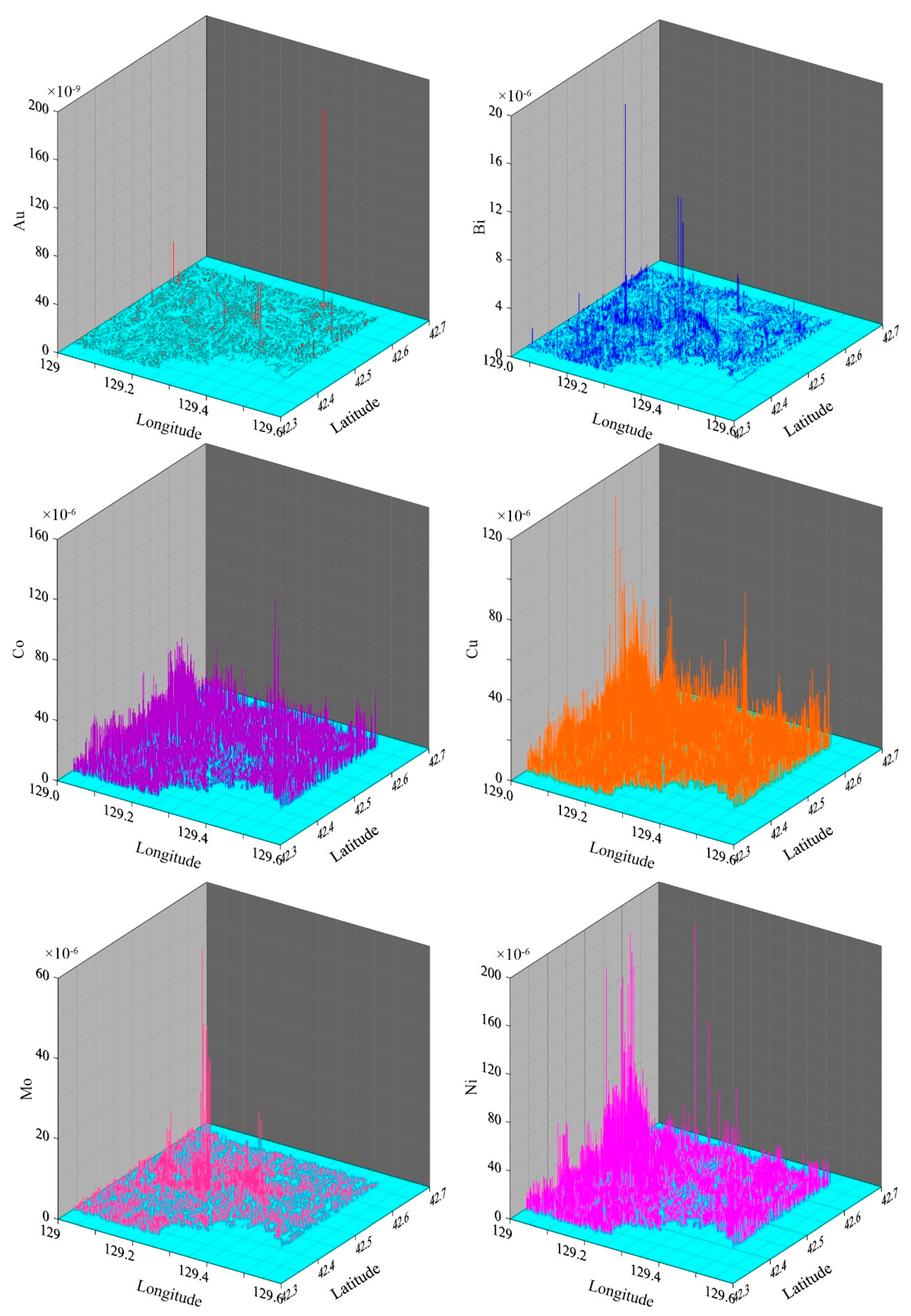
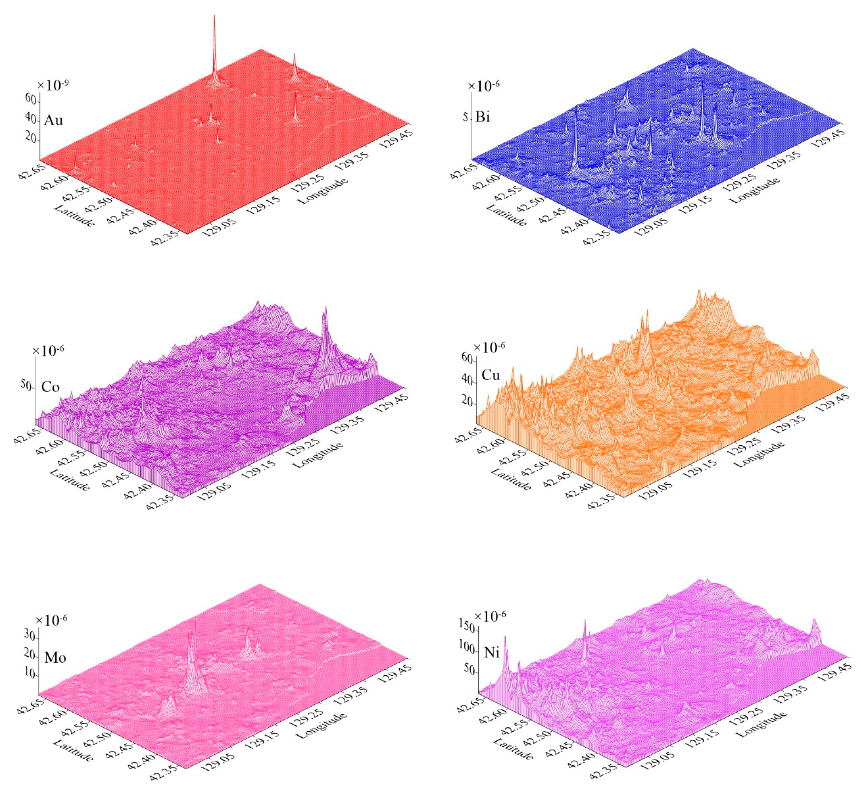
2.1. Geological and Geochemical Data

Geological and geochemical data for mineral prospectivity mapping came from the Digital Geological Survey recently conducted in the study area, which belongs to China’s New-Round Land Resources Survey Project [24]. The research group from Jilin University carried out field work in the study area and collected the data of geological structures, metamorphic rocks, magmatic rocks, sedimentary rocks, and mineral deposits, and saved the data in the MAPGIS system developed by the China University of Geosciences (Wuhan, China). At the same time, the research group completed the stream sediment survey in the study area, which was conducted in accordance with the Geochemical Survey Criteria (No. DZ/T0011-91), covering 1320 km² with a sampling density of 1–2 samples per 0.25 km². The concentrations of 13 elements in each stream sediment sample were analyzed and tested by the Inner Mongolia Mineral Experiment Institute, China. The concentration of Au was analyzed by atomic absorption spectrometry (AAS), the concentrations of Hg and As were analyzed by atomic fluorescence spectrophotometry (AFS), and the concentrations of Ag, Sb, Mo, W, Cu, Pb, Zn, Bi, Ni, and Co were analyzed by inductively coupled plasma mass spectrometry (ICP-MS).

Geological data were preprocessed in MAPGIS and further processed in the MapInfo software platform. Firstly, the projection coordinates of the geological maps were converted into longitude and latitude coordinates, and then into MapInfo tables. Finally, known mineral deposits, regional faults, different geological formations, and different magmatic rocks as well as their boundaries, were extracted from the geological data in the MapInfo software platform as potential evidence layers. The regional faults and magmatic rock boundaries were transformed into areal entities by buffering them to the optimal width in the MapInfo software platform. Each potential evidence layer is saved as a MapInfo Interchange file, which is the input data for the Python program developed by Yongliang Chen (see Supplementary Materials). The Python program then generated a layer of 200 × 134 unit cells, called the unit cell layer. Each cell is a rectangular area of 0.2282 × 0.2296 km², which satisfies the condition that there is no more than one known mineral deposit in one cell.

Geochemical data were preprocessed using Surfer 12. For each geochemical element, its concentrations collected from the 6999 valid sampling points were used to generate a 200 × 134 grid data by using Inverse Distance to a Power. In geochemical data interpolation, an integer value of 2 was used as the power value of the Inverse Distance to a Power, and the number of samples used to estimate a grid point value was between 8 and 64. Figure 1 shows the concentrations of Au, Bi, Co, Cu, Mo, and Ni collected from the 6999 valid sampling locations in the study area. The concentrations of the remaining seven elements are not shown here because they were not selected for mineral prospecting mapping in Section 3.2. Figure 2 shows the interpolated data of Au, Bi, Co, Cu, Mo, and Ni produced by the Inverse Distance to a Power in Surfer 12. By comparing Figure 1 and Figure 2, it can be found that the spatial distribution of element concentrations in the interpolated data is consistent with that in the vertical bar charts. Therefore, it is feasible to interpolate the geochemical data using Inverse Distance to a Power.

The grid map of each element generated above is consistent with the unit cell layer generated previously. Each grid point represents the corresponding unit cell in the unit cell layer. A grid point (unit cell) is defined as a true positive point if the cell represented by the grid point contains a known mineral deposit. Thus, the number of the true positive points defined in the study area is equal to the number of known mineral deposits. Except for these grid points which are defined as true positive points, all other grid points in the study area are defined as true negative points. The true positive and negative grid points defined in this section (Figure 3a) are hereafter used as the ground truth data to evaluate the performances of OCSVMs in subsequent sections.

The geological and geochemical evidences, spatially associated with known mineral deposits, were selected and converted into binary evidence map layers and used as the input data of OCSVM models. Binary geological evidences were selected by using the Youden index to evaluate spatial relationships between the geological evidences and known mineral deposits [13,14,21,22,23]. Continuous geochemical evidences were selected by statistically testing whether there exists significant spatial relationships between the geochemical evidences and the known mineral deposits [13,14,21,22,23]. The continuous geochemical evidences selected for mineral prospectivity mapping were then optimally converted into binary geochemical evidence layers by using the Youden index to evaluate the spatial relationship between the converted geochemical evidences and the known mineral deposits [13,14,21,22,23]. Figure 3b–r shows the 17 binary evidence maps selected for mineral prospectivity mapping in this study.

2.2. Receiver Operating Characteristic (ROC) Curve, Area under the Cuve (AUC), and Youden Index

The ROC curve of a continuous indicator is a graphical representation of the relationship between the continuous indicator and a binary target variable. Assuming that a study area has n grid points, the target variable divides the n grid points into true positive points and true negative points. A threshold is used to convert a continuous indicator into a binary indicator, which divides the n grid points into predicted positive points and predicted negative points. According to Chen and Wu [22], these classification results can be used to calculate benefit (that is, the percentage of the true positive points that are correctly predicted as positive points) and cost (that is, the percentage of the true negative points that are wrongly predicted as positive points). The computed benefits and costs vary with threshold. The ROC curve can represent the curve of benefit changing with cost under different threshold settings. A point on the ROC curve represents a threshold, and its vertical and horizontal coordinates represent the corresponding benefit and cost, respectively. The higher the relationship is between the continuous indicator and the binary target variable, the closer the ROC curve is to the upper left corner of the ROC space.

The AUC value of a continuous indicator is the area under the ROC curve of the continuous indicator, and it is a quantitative expression of the relationship between the continuous indicator and the binary target variable. Its value is in the range of 0.5 to 1, which corresponds respectively to the random and deterministic relationships between the continuous indicator and the binary target variable. Assume that there are t_p true positive and t_n true negative points in the study area. According to Chen [21], the AUC value of the continuous indicator can be expressed as

$$\mathrm{AUC}=\frac{1}{t_p{t}_n}{\displaystyle {{\displaystyle \sum }}_{i=1}^{t_p}}{\displaystyle {{\displaystyle \sum }}_{j=1}^{t_n}}\phi \left(f\left({\mathit{x}}_i\right),f({\mathit{y}}_j\right))$$

(1)

with

$$\phi \left(f\left({\mathit{x}}_i\right),({\mathit{y}}_j)\right)=\{\begin{array}{c}1,f({\mathit{x}}_i)>f\left({\mathit{y}}_j\right)\\ 0.5,f({\mathit{x}}_i)=f({\mathit{y}}_j\\ 0,f({\mathit{x}}_i)<f\left({\mathit{y}}_j\right)\end{array}).$$

where $f({\mathit{x}}_i)$ (i = 1, 2, …, p) represents the observed value of the continuous indicator at the ith true positive point, and $f({\mathit{y}}_j)$ (j = 1, 2, …, q) represents the observed value of the continuous indicator at the jth true negative point.

AUC is a random variable, which can be used to construct the following random variable Z_AUC that conforms to the standard normal distribution [21]:

$$Z_{AUC}=\frac{AUC-0.5}{S_{AUC}}$$

(2)

where S_AUC is the standard deviation of AUC, which can be calculated by

$$S_{\mathrm{AUC}}=\sqrt{\frac{AUC\left(1-AUC\right)+\left(t_p-1\right)\left(\frac{AUC}{2-AUC}-AU{C}^2\right)+\left(t_n-1\right)\left(\frac{2AU{C}^2}{1+AUC}-AU{C}^2\right)}{t_p{t}_n}}$$

(3)

Z_AUC can be used to test whether there is a significant difference between the AUC value and 0.5 at the significance level of α = 0.05 [13,14,21,22,23]. According to the unit normal loss function, at the significance level of α = 0.05, the critical value of Z_UAC is 1.96. If the Z_AUC value calculated by Equation (2) is greater than the critical value of 1.96, the probability of a significant difference between the AUC value and the value of 0.5 is not less than 0.95.

The Youden index of a binary indicator is the quantitative expression of the relationship between the binary indicator and a binary target variable. It is defined as benefit minus cost (i.e., the difference between the vertical coordinate and the horizontal coordinate of a point on the ROC curve) [22]. The Youden index is between −1 and +1, respectively, representing the deterministic negative and positive relationships. When the Youden index is close to zero, it means that there is little relationship between the binary indicator and the binary target variable.

In mineral prospectivity mapping, ROC curves and AUC values can be used to optimally select continuous evidence layers and to evaluate the performances of mineral prospectivity mapping methods [13,14,21,22]. The Youden index can be used to optimally select binary evidence map layers, as well as to determine the optimal threshold of a continuous evidence layer and the optimal buffering width of a linear evidence map layer [13,14,21,22].

2.3. OCSVM

Assume that m binary evidence layers are used for mineral prospectivity mapping in a study area of n unit cells. Data matrix $\left\{{\mathit{x}}_1,{\mathit{x}}_2,\cdots ,{\mathit{x}}_n\right\}$ represents the observed evidence data of the n unit cells in the study area. Each column vector ${\mathit{x}}_i={\left(x_{i1},x_{i2},\cdots ,x_{im}\right)}^T$ represents the observed values of the m evidence layers in the ith unit cell. Mapping mineral prospectivity using OCSVM is a binary classification process that classifies the n unit cells into single-class and outliers. An initialization parameter μ (0 < μ ≤ 1) is used to control the percentage of outliers among the n unit cells, that is, the n unit cells contain no more than $\mu n$ outliers. Outliers usually account for only a small proportion of all the cells in the study area and are considered as mineral targets in mineral prospectivity mapping [13].

In OCSVM, the support vector machine (SVM) theory is used to estimate a hyperplane that maximumly separates single-class and outliers [2]. Due to the nonlinear separability between single-class and outliers, the following Gaussian kernel [25] is usually used in OCSVM:

$$K\left({\mathit{x}}_i,{\mathit{x}}_j\right)=\exp \left(-\Vert {\mathit{x}}_i-{\mathit{x}}_j\Vert {}^2/{\sigma }^{-2}\right)$$

(4)

where ${\mathit{x}}_i$ and ${\mathit{x}}_j$, (i, j = 1, 2, …, n), are respectively the ith and jth unit cells, and $\sigma$ is the standard deviation of a Gaussian distribution, which is another initialization parameter of OCSVM.

The data set $\left\{{\mathit{x}}_1,{\mathit{x}}_2,\cdots ,{\mathit{x}}_n\right\}$ is used to train the OCSVM model initialized with the parameters μ and $\sigma$. According to the trained OCSVM model, the anomaly score of each unit cell is calculated by

$$f\left(\mathit{x}\right)={\displaystyle {{\displaystyle \sum }}_{i=1}^n}{\alpha }_i\left[K\left({\mathit{x}}_i,{\mathit{x}}_j\right)-K\left({\mathit{x}}_i,\mathit{x}\right)\right],j\in \left(1,2,\dots ,n\right)$$

(5)

where $f\left(\mathit{x}\right)$ is the anomaly score of cell x that denotes the degree of cell x being an outlier [13], ${\alpha }_i\left(i=1,2,\dots ,n\right)$ is the Lagrange parameter, $K\left(·,·\right)$ is the Gaussian kernel.

The initialization parameters μ and σ directly affect the performance of the OCSVM model for mineral prospectivity mapping [13]. Determining the optimal values of the parameters μ and σ to improve the performance of OCSVM can be solved by combining the OCSVM model with the bat algorithm.

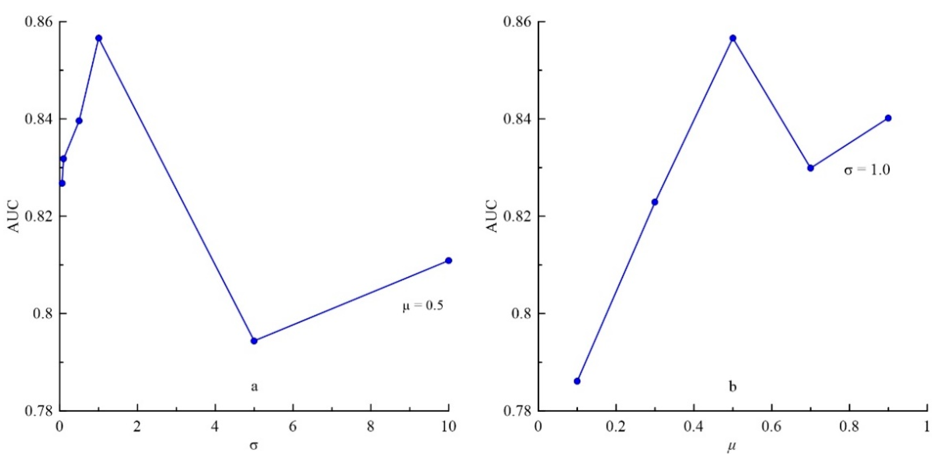
2.4. Bat-Optimized OCSVM

The bat algorithm is a heuristic search algorithm that simulates bats using sonar to detect prey and avoid obstacles. It maps L individuals in the bat population to L feasible solutions in a d-dimensional problem space, and uses the flying process of a bat in search for prey to simulate the optimization search process. The fitness value of solving the problem is used to evaluate the position of the bat, and the evolutionary process of survival of the fittest is used to simulate the iterative search process of the better feasible solution instead of the worse feasible solution. The bat algorithm dynamically controls the conversion between local search and global search to avoid the algorithm falling into the local optimum, and has good global convergence and superior performance in solving large-scale target optimization problems [17,18,19,20].

The bat algorithm is controlled by the following parameters: (a) L controlling the size of the bat population, (b) T controlling the number of iterations, (c) α and γ controlling convergence speed, (d) A controlling sound loudness, (e) r controlling sound emission rate, and (f) f and λ controlling the detectable range. According to Yang and Gandomi [17], the values of A, r, and f can be set between 0 and 1, and the values of α and γ can be simply set to α = γ = 0.9. A_min = 0 means that a bat has just found the target and temporarily stops making any sound, and r_min = 0 and r_max = 1 respectively represent no pulse and the maximum emission rate. f_min = 0 ≤ f ≤ 1 = f_max corresponds to λ_max ≥ λ ≥ λ_min. λ_max represents the detectable range, and adjusting it only needs to change f because λ × f is constant [16,17].

Each bat starts its heuristic search from a random location z_l in the d-dimensional search space after its loudness A_l, emission rate r_l, and frequency f_l are randomly initialized. Each bat l flies randomly with velocity v_l at location z_l, searching for prey with a fixed frequency f_l, varying wavelength λ_l and loudness A_l, and automatically adjusts wavelength λ_l according to the degree at which it is approaching the prey [16,17].

At each iteration t (0 ≤ t < T), a global search process is first conducted and the flying speed and spatial location of each bat are updated. The spatial coordinates of each bat l (0 ≤ l < L) is used to calculate the fitness value of the objective function, and then the spatial location corresponding to the largest fitness value is selected as the current optimal location ${\mathit{z}}_{*}$. According to Yang [16], the ${\mathit{v}}_l^t$ and ${\mathit{z}}_l^t$ are updated as follows:

$$f_l=f_{\min }+\left(f_{\max }-f_{\min }\right)\beta$$

(6)

$${\mathit{v}}_l^t={\mathit{v}}_l^{t-1}+\left({\mathit{z}}_l^t-{\mathit{z}}_{*}\right)f_l$$

(7)

$${\mathit{z}}_l^t={\mathit{z}}_l^{t-1}+{\mathit{v}}_l^t$$

(8)

where β ∈ [0, 1] is a random number drawn from a uniform distribution, ${\mathit{z}}_{*}$ is the current optimal location, and t is iteration number.

After the global search process described above, a local search is then performed around the current best location. According to Yang [16], during the local search, the new location is generated by the following local random walk and tested to see if it is the best among all the locations:

$${\mathit{z}}_{\mathrm{new}}={\mathit{z}}_{\mathrm{best}}+\mathit{\epsilon }\langle A^t\rangle$$

(9)

where ε ∈ [–1, 1] is a d-dimensional random vector, and $\langle A^t\rangle$ is the average loudness of the L bats at iteration t.

At the end of each iteration t, the loudness A_l and the emission rate r_l of each bat l are updated accordingly as follows:

$$A_l^{t+1}=\alpha A_l^t,r_l^{t+1}=r_l^0\left[1-\exp \left(-\gamma t\right)\right]$$

(10)

where α = γ = 0.9 are constants [16,17].

The process of updating the velocities and the locations of bats is somewhat similar to that of PSO [20]. The pace and range of the movement are basically controlled by the frequency, just like the movement of the virtual birds in PSO. To some extent, the bat algorithm can be regarded as a balanced combination of PSO and the intensive local search governed by the frequency tuning ability and the variables of loudness and pulse rate. The loudness and pulse rate that influence the balance need to be updated in each iteration. However, PSO is slightly different from the global search process of the bat algorithm. In PSO, the velocity of each bird is updated by adding random perturbation to the optimal position of the bird and the optimal position of the population. While during the global search process of the bat algorithm, the velocity of each bat is updated according to the spatial difference between the current position of the bat and the current optimal position of the population. First the frequency of each bat is updated, and then the velocity of the bat is updated by adding the product of the spatial difference and the frequency. In both PSO and the global search process of the bat algorithm, the velocity of an individual is taken as the step length of updating the location of the individual.

In the bat-optimized OCSVM model, the search space of the bat algorithm is a two-dimensional space of which the coordinate axes are composed of μ and σ. The search range of the bat population is defined as (0 < μ ≤ 1) and (0 < σ < c). Here c is a positive constant given by the user. The fitness value maximized by the iterative search process of the bat algorithm is the AUC value of the OCSVM model. The iterative search process starts from L random locations within the search space. At each iteration, the two coordinates of the spatial location occupied by each bat are used as the values of μ and σ to initialize the OCSVM model, and then the model is trained on the data $\left\{{\mathit{x}}_1,{\mathit{x}}_2,\cdots ,{\mathit{x}}_n\right\}$. The anomaly score of each unit cell is calculated using Equation (5) based on the trained OCSVM model. Finally, the AUC value of the OCSVM model is calculated using Equation (1) based on the anomaly scores and the ground truth data defined in Section 2.1. The location corresponding to the largest AUC value is selected as the current optimal location, and the spatial location of each individual bat is updated using Equations (6) to (8). After the locations of all the bats having been updated, the local search is implemented around the current optimal location using Equation (9). The loudness and the emission rate of each bat are updated accordingly using Equation (10).

Table 1. The pseudo code of the bat-optimized one-class support vector machine (OCSVM) model.

The Algorithm for the Bat-Optimized OCSVM Model
Input:
Binary data {x1, x2, …, xn};
Binary ground truth data {d1, d2, …, dn}.
Output:
Anomaly scores {f(x1), f(x2), …, f(xn)}.
Algorithm:
Initialization ():
Randomly initialize the location and velocity of each bat zl and vl, (l = 1, 2, …, L);
Define pulse frequency fl at zl, (l = 1, 2, …, L);
Initialize emission rate rl and the loudness Al, (l = 1, 2, …, L).
Evaluation ():
Initialize the OCSVM model using zl, (l = 1, 2, …, L);
Train the OCSVM model on the binary data {x1, x2, …, xn};
Compute the anomaly score of unit cell i using Equation (5), (i = 1, 2, …, n);
Compute the AUC of the OCSVM model initialized by zl (l = 1, 2, …, L) using Equation (1).
While (t < T):
Adjust the frequency of each bat fl using Equation (6) (l = 1, 2, …, L);
Update the velocity and location of each bat zl and vl using Equations (7) to (8) (l = 1, 2, …, L); Call Evaluation ().
If (random < rl):
Select a location among the best locations;
Generate a local location around the selected best location;
Generate a new location according to Equation (9); Call Evaluation ().
$\mathrm{If}(\mathrm{random}<A_l\mathrm{and}\mathrm{the}\mathrm{AUC}\mathrm{for}{\mathit{z}}_l<\mathrm{the}\mathrm{AUC}\mathrm{for}{\mathit{z}}_{*}$):
Accept the new locations;
Increase rl and reduce Al according to Equation (10);
Rank the bats and find the current best ${\mathit{z}}_{*}$.
Output the results.

outlines the pseudo code of the bat-optimized OCSVM model.

3. Mapping Mineral Prospectivity

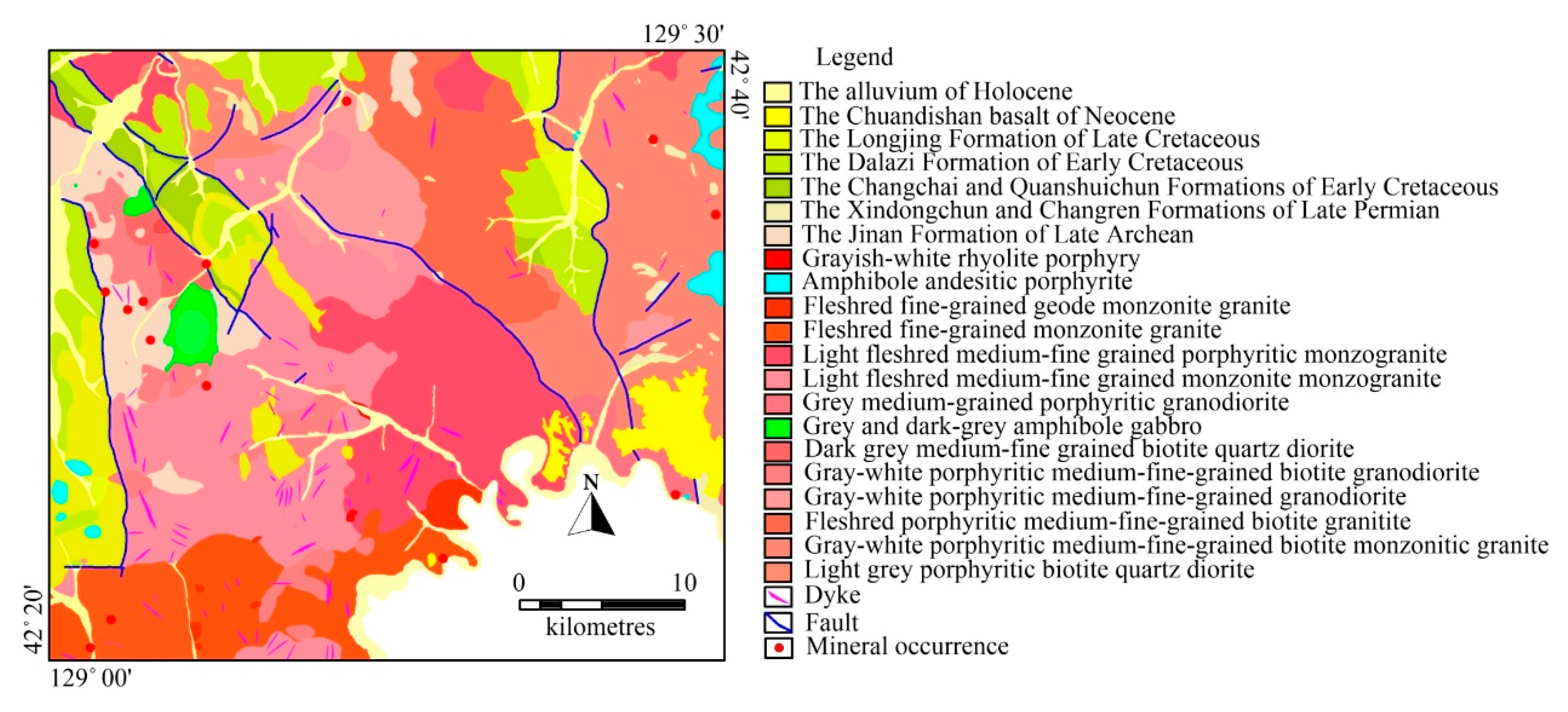
3.1. Geological Background and Mineralization

The study area is a complex tectonic belt superimposed between the Paleo-Asian tectonic domain and the Circum-Pacific tectonic domain, which has undergone the ancient Asian ocean evolution and the subduction of the Mesozoic Pacific plate [26,27,28]. The northwest-trending Gudonghe tectono-magmatic complex belt runs through the whole study area and controls the spatial distribution of major geological formations since the Late Paleozoic. Widely exposed magmatic rocks account for 69.58% of the whole study area. Granite, granodiorite, diorite, and gabbro are mainly magmatic rocks, forming widely exposed batholiths and stocks (Figure 4). Zircon U-Pb ages of diorites are 173–175 Ma [29], indicating that the magmatic rocks were formed during the Yanshan tectonic period. The exposed strata account for 29.44% of the total study area. The main strata are the Jinan Formation of Late Archean, the Xindongchun and Changren Formations of Late Permian, the Changchai, Quanshuichun, and Dalazi Formations of Early Cretaceous, the Longjing Formation of Late Cretaceous, the Chuandishan basalt of Neocene, and the alluvium of Holocene.

During the Yanshanian tectonic magmatism, a series of intermediate-acidic magmatic complexes were formed, which provided a continuous heat source and metallogenic materials for polymetallic mineralization [30]. There were 14 mineral deposits discovered in the study area. These mineral deposits are mainly hydrothermal and skarn type deposits which are closely related to multi-stage magmatic activities [30,31,32]. Most of the discovered mineral deposits are hosted in metamorphic rocks around or at the edges of magmatic intrusions (Figure 4). Regional structures, Archean formations, and the Yanshanian intermediate-acidic magmatic rocks are the three controlling factors for polymetallic mineralization.

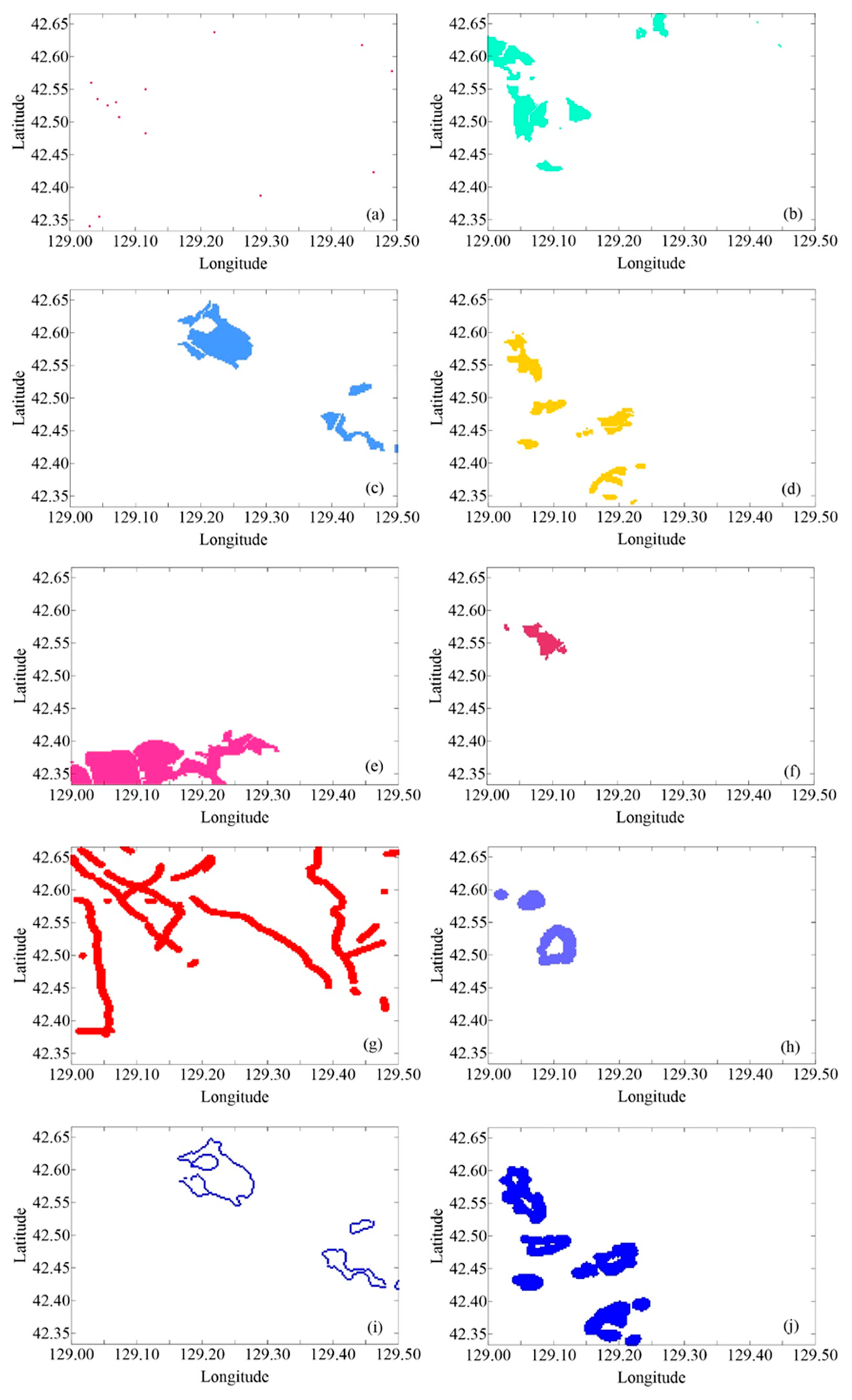
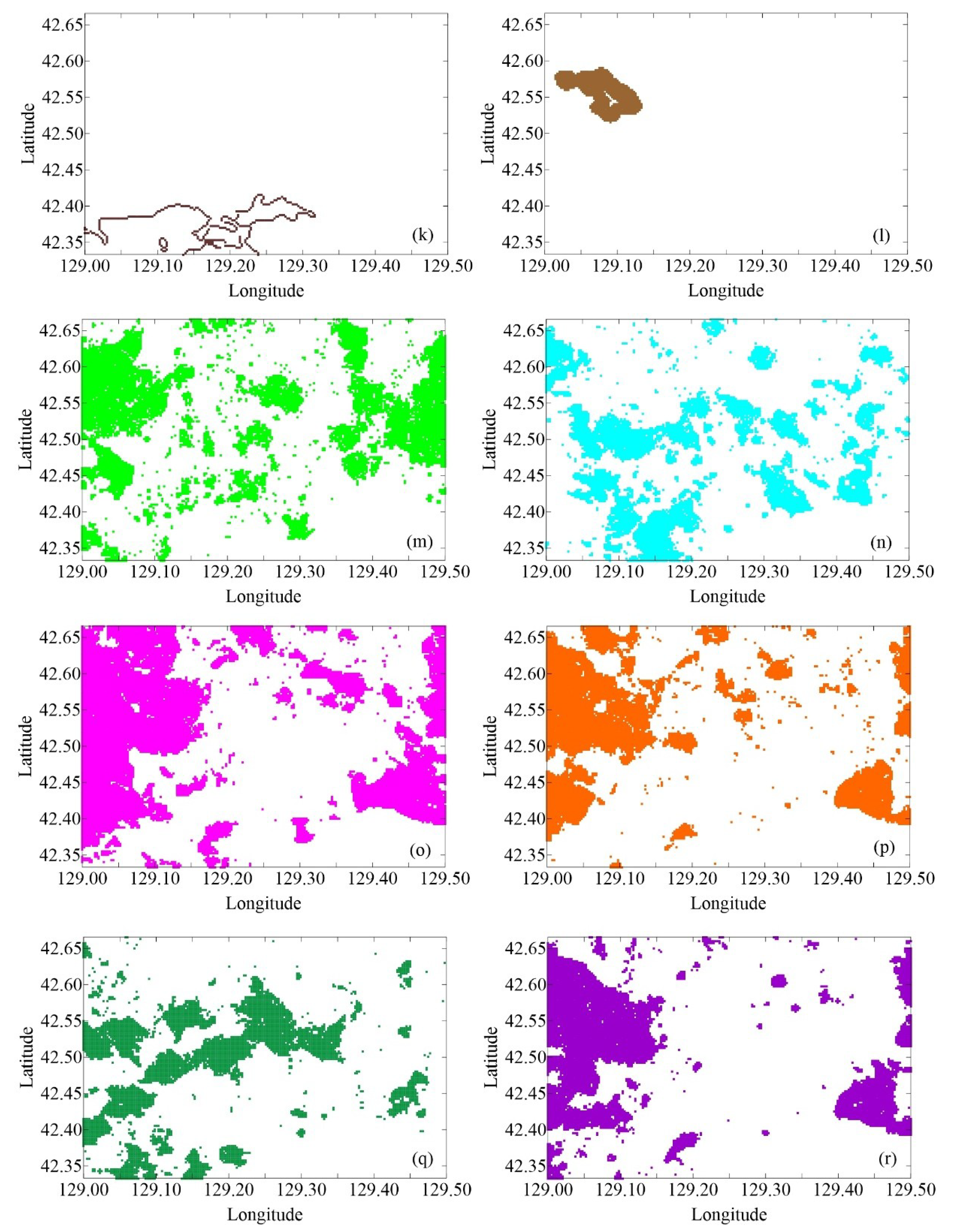
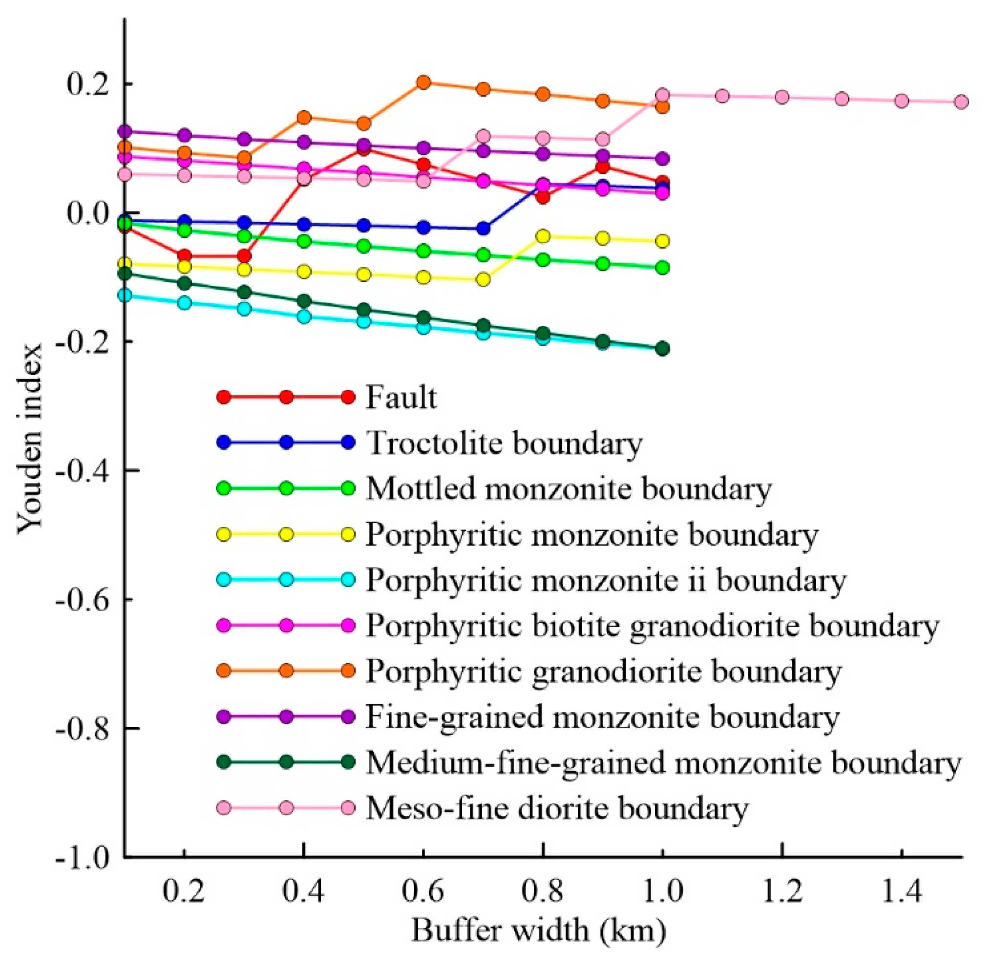
3.2. Evidence Map Layers

In this section, geological and geochemical evidence layers are selected for mapping mineral prospectivity. Firstly, the optimal buffer width of each linear geological evidence is determined by using the Youden index, and then the linear evidence is converted into areal evidence through buffering to the optimal buffer width. Finally, the Youden indices of all the geological evidences are calculated, and the geological evidences with Youden indices larger than the predefined threshold are selected for mapping mineral prospectivity. The AUCs and Z_AUCs of all the geochemical elements are calculated, and those elements with Z_AUCs greater than the critical value of 1.96 are selected for mapping mineral prospectivity. The selected elements are finally optimally converted into binary evidences using the Youden index.

Faults and the boundaries of magmatic intrusions are linear evidences for mineral prospectivity mapping, which need to be converted into areal evidences by buffering in the MapInfo software platform. The optimal buffer width of one linear evidence can be determined by evaluating the spatial relationship between the buffered evidence and known mineral deposits using the Youden index [13,14,21,22,23]. For a linear evidence, the optimal buffer width maximizes its Youden index, meaning that the linear evidence buffered to the optimal buffer width has the highest spatial relationship with known mineral deposits. In this study, ten types of linear evidences were extracted in the study area. Figure 5 shows the curves of the Youden indices of various linear evidences varying with buffer width. The maximum Youden index and optimal buffer width of each linear evidence is listed in

Table 2. The maximum Youden indices and optimal buffer widths of the 10 linear evidences.

Linear Evidence	MYI	OBW (km)
Regional structure	0.09887	0.5
Troctolite boundary	0.04405	0.8
Mottled monzonite boundary	−0.01642	0.1
Porphyritic monzonite boundary	−0.03696	0.8
Stage II porphyritic monzonite boundary	−0.1287	0.1
Porphyritic biotite granodiorite boundary	0.08729	0.1
Porphyritic granodiorite boundary	0.2019	0.6
Fine-grained monzonite boundary	0.1264	0.1
Medium-fine-grained monzonite boundary	−0.09409	0.1
Medium-fine-grained diorite boundary	0.1831	1.0

Note: MYI denotes the maximum Youden index; OBW denotes the optimal buffer width.

. The optimally buffered linear evidences were then used as areal evidences for mineral prospectivity mapping.

After the above buffer analysis, a total of 26 areal geological evidence layers were derived as potential evidence layers for mineral prospectivity mapping in the study area. The Youden index of each layer was calculated to select the evidence layer with a higher spatial relationship with known mineral deposits. Theoretically, as long as the Youden index of an evidence layer is greater than zero, the evidence is considered to be spatially associated with known mineral deposits. However, there is no way to statistically test whether this spatial relationship is significant. Therefore, it is better to use a threshold slightly larger than zero when selecting the geological evidence layers in mineral prospectivity mapping. In this study, the following 11 geological evidence layers were selected using a threshold value = 0.01: (a) the Jinan Formation of Late Archean, (b) porphyritic biotite granodiorite, (c) porphyritic granodiorite, (d) fine-grained monzonite, (e) medium-fine-grained diorite, (f) fault with 0.5 km buffer, (g) troctolite boundary with 0.8 km buffer, (h) porphyritic biotite granodiorite boundary with 0.1 km buffer, (i) porphyritic granodiorite boundary with 0.6 km buffer, (j) fine-grained monzonite boundary with 0.1 km buffer, and (k) medium-fine-grained diorite boundary with 1.0 km buffer. These geological evidence layers are consistent with the metallogenic controlling factors discussed in Section 3.1. The evidence layer (a) is the Archean metamorphic formation, the evidence layers (b) through (e) are the Yanshanian magmatic intrusions, the evidence layer (f) is the regional structure, and the evidence layers (g) through (k) are the boundaries of the Yanshanian magmatic intrusions.

Geochemical evidence layers are selected by using the AUCs and Z_AUCs discussed in Section 2.2. Equation (1) was used to calculate the AUC value of each element according to the preprocessed data in Section 2.1. Then, Equation (2) was used to estimate the Z_AUC value according to the AUC value. If the estimated value of Z_AUC is greater than the critical value of 1.96 at the significance level of 0.05, the AUC value is considered to be significantly different from the value of 0.5. This means that the concentrations of the element are significantly spatially correlated to the known mineral deposits. In other words, the higher the concentration of the element in unit cells, the more likely the unit cells contain known mineral deposits.

Table 3. Area under the curves (AUCs) and Z_AUCs for 13 elements.

Element	AUC	ZAUC	Element	AUC	ZAUC	Element	AUC	ZAUC
Ag	0.5268	0.3416	Cu	0.7222	2.8661	Sb	0.5802	1.0037
As	0.6195	1.4889	Hg	0.5949	1.1835	W	0.6561	1.9531
Au	0.6893	2.3958	Mo	0.7159	2.7727	Zn	0.6537	1.9217
Bi	0.6620	2.0295	Ni	0.7619	3.4986
Co	0.7007	2.5540	Pb	0.4327	–0.9248

lists the AUCs and Z_AUCs of 13 elements estimated in this study. As can be seen from Table 3, the Z_AUCs of Au, Co, Cu, Mo, Ni, and W are greater than the critical value of 1.96. Thus, the concentrations of these elements are significantly spatially correlated to the known mineral deposits.

According to the above statistical results, gold, Bi, Co, Cu, Mo, and Ni were selected as geochemical evidences for mineral prospectivity mapping. Among these elements, bismuth is an ore-forming associated element, and the other five elements are metallogenic elements. Thus, these statistical results are consistent with the mineralization characteristics of the study area. The optimal thresholds for extracting the concentration anomalies of the six elements were determined by evaluating the spatial relationship between the extracted anomalies and known mineral deposits using the Youden index. The higher the Youden index of the extracted anomalies (a binary map layer), the more likely the extracted anomalies spatially coincide with the known mineral deposits. The optimal threshold maximizes the Youden index of the extracted geochemical anomalies.

Table 4. The maximum Youden indices and optimal thresholds of the six indicator elements.

Element	MYI	OT	Element	MYI	OT	Element	MYI	OT
Au	0.3483	0.6421	Bi	0.3357	0.1996	Co	0.3989	7.3378
Cu	0.3889	11.0669	Mo	0.36406	1.1283	Ni	0.4715	10.5810

Note: MYI denotes maximum Youden index; OT denotes optimal threshold.

lists the maximum Youden indices and corresponding optimal thresholds of the six elements. Figure 6 shows the element concentration anomalies extracted from the grid data generated in Section 2.1. According to the extracted geochemical anomalies, six geochemical evidence layers were derived for mineral prospectivity mapping.

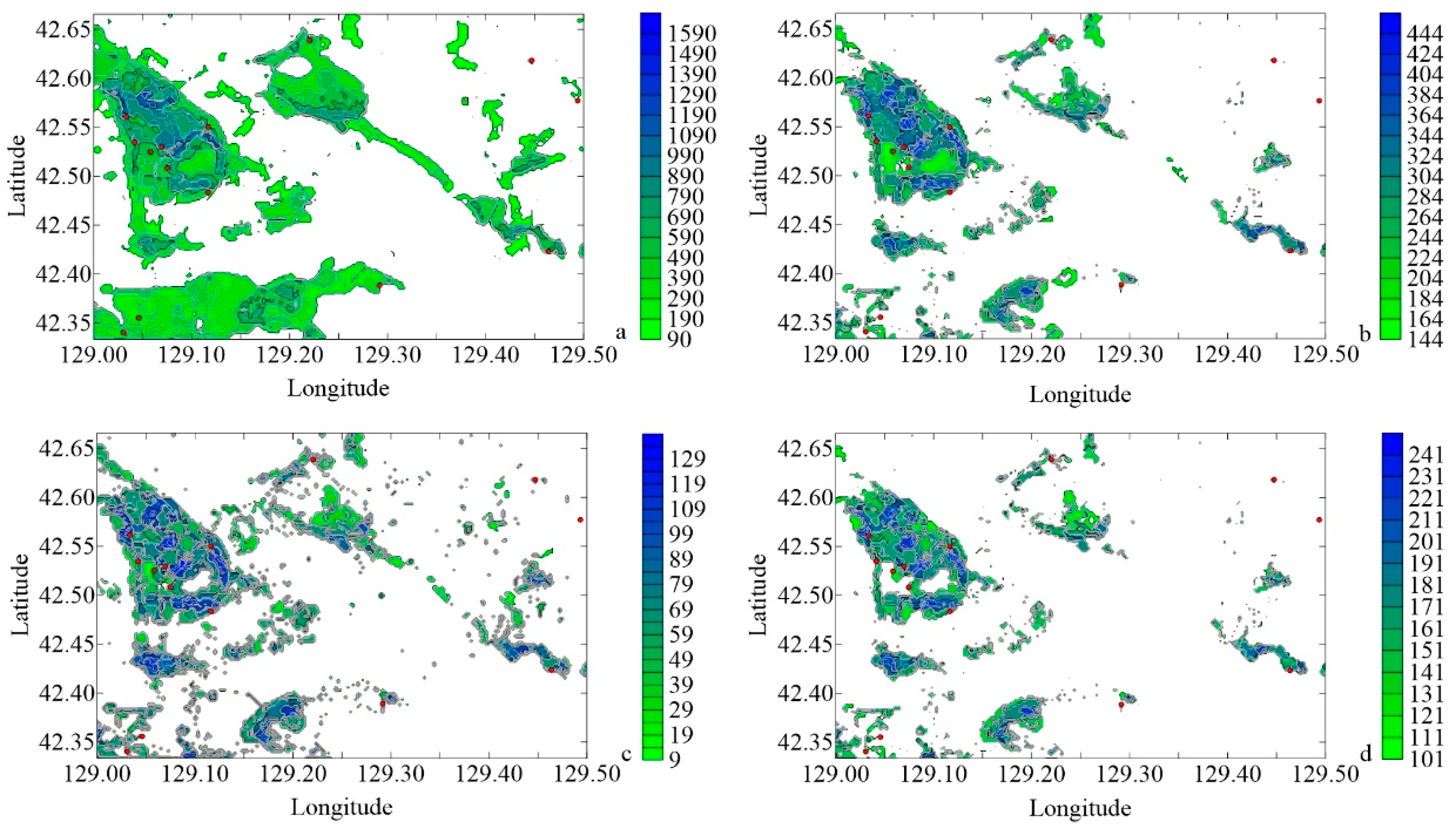
3.3. Mineral Target Extraction

In mineral prospectivity mapping, an initialized OCSVM model is trained on binary evidence data and then used to calculate the anomaly score of each unit cell. According to the anomaly scores of all the unit cells, geological anomalies are extracted by the optimal threshold determined by using the Youden index [13,14,21,22,23]. The extracted geological anomalies are usually closely spatially related to known mineral deposits. Therefore, these geological anomalies can be used as mineral targets [13,14,21,22,23]. The optimal threshold for separating geological anomalies is usually determined by selecting the threshold corresponding to the maximum Youden index from all the potential thresholds. In this study, the OCSVMs either initialized with the default parameters or optimized by both the trial and error method and bat algorithm which were used to map mineral prospectivity in the study area. The optimal threshold values were determined by maximizing the corresponding Youden indices.

The OCSVM model was first initialized using the default parameter values μ = 0.5 and σ = 1.0/17 and then trained on the evidence data. Here, 17 is the number of evidence layers used for mineral prospectivity mapping. The AUC value of the OCSVM initialized with the default parameters is 0.8268. The trial and error method was then used to determine the “optimal” parameters of OCSVM. Firstly, we set μ = 0.5, and then set σ respectively to σ = 0.0588, 0.1, 0.5, 1.0, 5.0, and 10.0. Here, μ = 0.5 and σ = 0.0588 are the default values of μ and σ. The OCSVM initialized with each pair of μ and σ was used to map mineral prospectivity. Figure 7a shows the curve of the AUC value of the OCSVM model changing with σ. It can be seen from Figure 7a that the OCSVM model has the highest AUC value at σ = 1.0. Therefore, σ = 1.0 was selected as the “optimal” value of σ, and then we set μ = 0.1, 0.3, 0.5, 0.7, and 0.9. The OCSVM model initialized with each of the five pairs of μ and σ was used to map mineral prospectivity. The variation of the AUC value of the OCSVM model with μ is shown in Figure 7b. According to Figure 7a,b, the “optimal” values of σ and μ are σ = 1.0 and μ = 0.5 respectively, and the corresponding maximum AUC value is 0.8567. The optimal threshold of the anomaly score was determined by using the Youden index and used to extract mineral targets. According to the value of the Youden index, the optimal threshold with respect to the maximum Youden index was selected from 1000 potential thresholds evenly distributed between the minimum and maximum values of anomaly scores. The optimal threshold for the common OCSVM model is optimal threshold OT0 = 89.8292 and the corresponding maximum Youden index is maximum Youden index MYI0 = 0.5092. The mineral targets extracted by the optimal threshold OT0 = 89.8292 are shown in Figure 8a. The optimal threshold for the “optimized” OCSVM is OT1 = 144.3031 and the corresponding maximum Youden index is MYI1 = 0.6214. The mineral targets extracted by the optimal threshold OT1 = 144.3031 are shown in Figure 8b.

In order to specify the search space of the bat population, the value ranges of μ and σ were empirically defined as (0, 1] and (0, 10], respectively. The eight initialization parameters of the bat algorithm were defined respectively as L = 20, T = 30, f_min = 0, f_max = 1, A_min = 0, A_max = 1, and α = γ = 0.9. Figure 9a shows that in the optimization process of the bat algorithm, as the number of iterations increases, the AUC value of the OCSVM model becomes larger and larger. It can be seen from Figure 9a that after 23 iterations, the bat algorithm converges to AUC = 0.8649. The corresponding optimal values of μ and σ are respectively μ = 0.4276 and σ = 1.7559. The optimal threshold determined by using the Youden index is OT2 = 9.2496, and the corresponding maximum Youden index is MYI2 = 0.5763. The mineral targets extracted by the optimal threshold OT2 = 9.2496 are shown in Figure 8c.

In order to compare the mineral prospectivity mapping results when different parameter values were used to initialize the bat algorithm, the initialization parameter values of the bat algorithm were changed to: L = 30, T = 20, f_min = 0, f_max = 1, A_min = 0, A_max = 1, and α = γ = 0.9. Figure 9b shows that in the optimization process of the bat algorithm, the AUC value of the OCSVM model increases with the increase of the number of iterations. It can be seen from Figure 9b that after 10 iterations, the bat algorithm converges to AUC = 0.8644. The corresponding optimal solution is μ = 0.4764 and σ = 1.3602. The optimal threshold determined by using the Youden index is OT3 = 101.4408, and the corresponding maximum Youden index is MYI3 = 0.5846. The mineral targets extracted by the optimal threshold OT3 = 101.4408 are shown in Figure 8d.

Figure 8a–d shows that the value ranges of anomaly scores generated by the four OCSVM models are quite different. However, these differences do not affect the validity of the OCSVM models in mineral prospectivity mapping, because we are only interested in the relative difference of anomaly scores between different unit cells and do not care about the absolute value of the anomaly score of a unit cell. The value range of the anomaly score is mainly affected by σ, and the smaller σ is, the larger it is. To illustrate the relationship between the value range of the anomaly score and σ, we set μ = 0.5, and then set σ = 0.05, 0.1, 0.5, 1.0, 5.0, 10.0, 50.0, 100.0, and 500.0, respectively. The OCSVM model initialized with μ = 0.5 and different values of σ was used to map mineral prospectivity. The corresponding minimum and maximum values of the anomaly score are listed in

Table 5. The minimum and maximum values of the anomaly score generated by the OCSVM initialized with different values of σ.

	σ	0.05	0.1	0.5	1.0	5.0	10.0	50.0	100.0	500.0
Score
Minimum		−300	−300	−200	−60	−5	−5	−5	−5	−5
Maximum		2000	1600	1200	460	95	95	95	95	95

Note: parameter μ = 0.5.

. The relationship between the value range of the anomaly score and σ can also be explained theoretically. Parameter σ is the responding width of the Gaussian kernel function in Equation (4). Reducing the value of σ is equivalent to amplifying the difference between samples in the kernel space. As a result, the value range of the anomaly score is enlarged. In order to make the anomaly scores generated by different OCSVM models have the same data change interval, the anomaly scores generated by OCSVM can be further transformed as follows:

$$\tilde{f}\left(x\right)=\frac{f\left(x\right)-\min \left\{f\left(x\right)\right\}}{\max \left\{f\left(x\right)\right\}-\min \left\{f\left(x\right)\right\}}$$

(11)

where $\tilde{f}\left(x\right)$ is the transformed anomaly score, $\min \left\{f\left(x\right)\right\}$ and $\max \left\{f\left(x\right)\right\}$ are the minimum and maximum values of $f\left(x\right)$. The transformed anomaly score $\tilde{f}\left(x\right)$ is between 0 and 1. This transformation does not affect the performance of OCSVM in mineral prospectivity mapping.

4. Results

In this section, the mineral prospectivity mapping results in Section 3.3 was statistically evaluated. The ROC curve and AUC value were used to evaluate whether the anomaly scores generated by the OCSVM model in Section 3.3 are effective for predicting known mineral deposit locations in the study area. The ROC curve and the AUC value are respectively the graphical and overall representations of the spatial relationship between the anomaly scores and known mineral deposit locations [13,14,21,22,23]. The higher the spatial relationship is between the anomaly scores and known mineral deposit locations, the more effective the anomaly scores are in predicting the known mineral deposit locations. Accordingly, the closer the ROC curve of the anomaly scores is to the upper left corner of the ROC space, the closer the AUC value of the anomaly scores is to 1.0, indicating that the corresponding OCSVM model performs better in mineral prospectivity mapping. The AUC value can be used to further estimate the Z_AUC value, and check whether there is a significant spatial relationship between the anomaly scores and the known mineral deposit locations [13,14,21,22,23].

In this study, each of the 1000 potential thresholds evenly distributed between the minimum and maximum anomaly scores was used to extract geological anomalies from the unit cell population. The benefit and cost for the threshold were calculated according to the predicted positive (anomaly) and negative (normal) points (unit cells) as well as the ground truth data defined in Section 2.1. The ROC curve of the anomaly scores was finally drawn based on the 1000 pairs of costs and benefits. Figure 10 shows the ROC curves of the anomaly scores generated by the common and optimized OCSVMs. As can be seen from Figure 10, although the four ROC curves are intersected, the ROC curves of the optimized OCSVMs slightly dominate that of the common OCSVM in the ROC space. Therefore, according to the ROC curve analysis results, the optimized OCSVMs perform better than the common OCSVM in mineral prospectivity mapping.

The AUC values of the common and optimized OCSVMs were calculated using Equation (1) according to the anomaly scores and the ground truth data defined in Section 2.1. The Z_AUCs for the common and optimized OCSVMs were calculated using Equation (2).

Table 6. Performance evaluation statistics of the common and optimized OCSVM models.

Statistics	AUC	ZAUC	MYI	OT	PGA (%)	Benefit (%)	PMT (s)
OCSVM0	0.8268	4.8032	0.5092	89.8292	29.61	93	47.73
OCSVM1	0.8567	5.6029	0.6214	144.3031	18.66	86	n/a
OCSVM2	0.8649	5.8639	0.5763	9.2496	19.84	93	24,856.56
OCSVM3	0.8644	5.8483	0.5846	101.4408	14.22	86	39,314.25

Note: MYI denotes maximum Youden index; OT denotes optimal threshold; PGA denotes the percentage of geological anomalies; PMT denotes program modeling time; OCSVM0 denotes the OCSVM initialized with the default parameters; OCSVM1 denotes the OCSVM optimized by trial and error; and OCSVM2 and OCSVM3 denote the OCSVMs optimized respectively by the bat algorithm with L = 20, T = 30 and the bat algorithm with L = 30, T = 20.

lists the performance evaluation statistics of the common and optimized OCSVMs in mineral prospectivity mapping.

As can be seen from Table 6, the AUC value of the common and trial and error-optimized OCVSMs are 0.8268 and 0.8566, while the bat-optimized OCSVMs are respectively 0.8649 and 0.8644. Therefore, according to the estimated AUC values, the bat-optimized OCSVMs perform slightly better than the common and trial and error-optimized OCSVMs in mineral prospectivity mapping. The Z_AUCs of the common and trial and error-optimized OCSVMs are 4.8032 and 5.6029, and the Z_AUCs of the bat-optimized OCSVMs are 5.8639 and 5.8483, respectively. These four Z_AUCs are far higher than the critical value of 1.96. Therefore, both the common and optimized OCSVMs are significantly effective in predicting the known mineral deposit locations in the study area. In other words, the mineral targets predicted by the common and optimized OCSVMs are significantly spatially associated with known mineral deposits in the study area.

According to the anomaly scores generated by the common and trial and error-optimized OCVSMs, the optimal thresholds OT0 = 89.83 and OT1 = 144.3031 extract 29.61% and 18.66% of the study area as mineral targets respectively, and 93% and 86% of known mineral deposits are located in these mineral targets. According to the anomaly scores generated by the bat-optimized OCVSMs, the optimal threshold OT2 = 9.2496 and OT3 = 101.4408 extract 19.84% and 14.22% of the study area as mineral targets respectively, and 93% and 86% of known mineral deposits are located in the corresponding mineral targets. Therefore, we have 0.93/0.2961 = 3.1408 < 0.86/0.1866 = 4.6088 < 0.93/0.1984 = 4.6875 < 0.86/0.1422 = 6.0478. We call these ratios unit benefit values. Therefore, the bat-optimized OCSVMs perform slightly better than the common and trial and error-optimized OCSVMs in mineral prospectivity mapping.

By comparing Figure 8 and Figure 4, it can be concluded that the mineral targets predicted by the common and optimized OCSVMs spatially coincide with the Late Archean Jinan Formation and the Yanshanian magmatic rocks (including fleshy red fine-grained monzonite, gray-white porphyritic biotite granodiorite, and porphyritic monzonite). The mineral targets predicted are spatially controlled by the regional northwest-trending structures. These results are consistent with the regional geological characteristics of the study area discussed in Section 3.1.

5. Discussion

When the bat-optimized OCSVMs are used to map mineral prospectivity, the parameters L, T, f_min, f_max, A_min, A_max, α, and γ need to be defined for the bat algorithm. Among these parameters, only L and T maybe significantly affect the performance of the bat-optimized OCSVM. The other six parameters are usually defined as the default values suggested by Yang and Gandomi [17].

In order to test the influences of L and T on the performance of bat-optimized OCSVM, the performance evaluation statistics listed in Table 6 and the ROC curves shown in Figure 10 were used to compare the performances of the two bat-optimized OCSVMs. As can be seen from Table 6 and Figure 10, although the performance evaluation statistics of the two models are different, the ROC curves of the two models shown in Figure 10 are almost coincident in the ROC space, and the AUC values of the two models (0.8649 and 0.8644) are approximately equal. The Pearson’s correlation coefficient between the anomaly scores generated by the two models is R = 0.9792 (the number of samples is 18,905), indicating a high correlation between the anomaly scores generated by the two models. As can be seen from Figure 9, the two iterative processes of the bat algorithm converge to AUC = 0.8644 and AUC = 0.8649, respectively. Therefore, the values of L and T have no significant influence on the performance of the bat-optimized OCSVM in mineral prospectivity mapping. As long as L and T values are within an appropriate range (20 ≤ L, T ≤ 30), the bat-optimized OCSVM can achieve similar good results in mineral prospecting mapping.

The bat algorithm initialized by L = 20, T = 30, f_min = 0, f_max = 1, A_min = 0, A_max = 1, and α = γ = 0.9 was used to repeatedly optimize OCSVM parameters three times, to verify whether the bat algorithm can always converge to the global optimum. The results show that in each data modeling process, the bat algorithm converges to the same maximum AUC = 0.8649. Therefore, the bat algorithm can generally converge to the global maximum in OCSVM parameter optimization in mineral prospectivity mapping.

In this study, the bat-optimized OCSVM is established to map mineral prospectivity. The model can also be used to solve other similar anomaly detection problems. For example, the bat-optimized OCSVM can be established to detect multivariate geochemical anomalies. The application condition of the model is that there are a certain number of known mineral deposits in the study area to define the ground truth data, so that the ROC curve analysis can be implemented.

It should be pointed out that compared with the common OCSVM, the bat-optimized OCSVM needs more time to search for the optimal parameter values of OCSVM. This leads to the low efficiency of the bat-optimized OCSVM in data modeling. It can be seen from this study that the data modeling time of the bat-optimized OCSVM 1 (24856.56 s) and the bat-optimized OCSVM 2 (39314.25 s) is much longer than that of the common OCSVM (47.73 s).

6. Conclusions

I. A bat-optimized one-class support vector machine is developed by combining one-class support vector machine with the bat algorithm. The combined model can automatically optimize the parameter values of a one-class support vector machine, so as to improve the performance of the model in mineral prospectivity mapping. The method proposed in this paper only needs to set the search space, and then the algorithm automatically searches the optimal parameters. Compared to the trial and error method, the proposed method has more opportunities to find the global optimal parameters.

II. The bat-optimized one-class support vector machine requires a certain number of known mineral deposits in the study area, which can be used to define the true positive and negative points (cells), and be used as the ground truth data for the receiver operating characteristic curve analysis. As long as a study area meets this application condition, the bat-optimized model can also be established to solve other similar anomaly detection problems in geosciences, such as multivariate geochemical anomaly detection. The bat-optimized one-class support vector machine can be used as a semi-supervised machine learning model to handle anomaly detection problems in other application fields.

III. The case study shows that the AUC values of the bat-optimized one-class support vector machine models are greater than those of the common and trial and error-optimized one-class support vector machine models. The mineral targets predicted by the bat-optimized one-class support vector machine models have larger unit benefit values compared to those predicted by the common and trial and error-optimized one-class support vector machine models. Therefore, the bat-optimized one-class support vector machine models are a mineral prospectivity mapping method with high performance.

IV. The Z_AUC values of both the common and optimized one-class support vector machine models calculated in the case study are much higher than the critical value 1.96 at the significant level of 0.05. Therefore, the mineral targets predicted by both the common and optimized one-class support vector machine models are significantly spatially associated with known mineral deposits in the study area.

V. The mineral targets predicted by both the common and optimized one-class support vector machine models are spatially consistent with geological and metallogenic characteristics of the study area. The predicted mineral targets spatially coincide with the Late Archean Jinan Formation and the Yanshanian magmatic rocks, and are obviously controlled by northwest-trending structures. The two formations and the structures are the three regional mineralization controlling factors in the study area.

References

1. Hayton, P.; Schӧlkopf, B.; Tarassenko, L.; Anuzis, P. Support vector novelty detection applied to jet engine vibration spectra. In Proceedings of the Advances in Neural Information Processing Systems 13 (NIPS’ 2000), Denver, CO, USA, 27 November–2 December 2000; pp. 946–952. [Google Scholar]
2. Schӧlkopf, B.; Platt, J.; Shawe-Taylor, J.; Smola, A.; Williamson, R. Estimating the support of a high-dimensional distribution. Neural Comput. 2001, 13, 1443–1471. [Google Scholar] [CrossRef]
3. Davy, M.; Godsill, S.J. Detection of abrupt spectral changes using support vector machines—An application to audio signal segmentation. In Proceedings of the International Conference on Acoustics, Speech, and Signal Processing (IEEE ICASSP-02), Orlando, FL, USA, 13–17 May 2002; pp. 1313–1316. [Google Scholar]
4. Lengelle, R.; Capman, F.; Ravera, B. Abnormal events detection using unsupervised one-class SVM–Application to audio surveillance and evaluation. In Proceedings of the 8th IEEE International Conference on Advanced Video and Signal-Based Surveillance (AVSS 2011), Klagenfurt, Austria, 30 August–2 September 2011; pp. 124–129. [Google Scholar]
5. Shin, H.J.; Eom, D.H.; Kim, S.S. One-class support vector machines—An application in machine fault detection and classification. Comput. Ind. Eng. 2005, 48, 395–408. [Google Scholar]
6. Mahadevan, S.; Shah, S.L. Fault detection and diagnosis in process data using one-class support vector machines. J. Process Control 2009, 19, 1627–1639. [Google Scholar] [CrossRef]
7. Fergani, B.; Davy, M.; Houacine, A. Speaker diarization using one-class support vector machines. Speech Commun. 2008, 50, 355–365. [Google Scholar] [CrossRef]
8. Mourão-Miranda, J.; Hardoon, D.R.; Hahn, T.; Marquand, A.F.; Williams, S.C.R.; Shawe-Taylor, J.; Brammer, M. Patient classification as an outlier detection problem: An application of the One-Class Support Vector Machine. NeuroImage 2011, 58, 793–804. [Google Scholar] [CrossRef] [Green Version]
9. Strobbe, T.; Wyffels, F.; Verstraeten, R.; De Meyer, R.; Van Campenhout, J. Automatic architectural style detection using one-class support vector machines and graph kernels. Autom. Constr. 2016, 69, 1–10. [Google Scholar] [CrossRef]
10. Roodposhti, M.S.; Safarrad, T.; Shahabi, H. Drought sensitivity mapping using two one-class support vector machine algorithms. Atmos. Res. 2017, 193, 73–82. [Google Scholar] [CrossRef]
11. Saari, J.; Strömbergsson, D.; Lundberg, J.; Thomson, A. Detection and identification of windmill bearing faults using a one-class support vector machine (SVM). Measurement 2019, 137, 287–301. [Google Scholar] [CrossRef]
12. Harrou, F.; Dairi, A.; Taghezouit, B.; Sun, Y. An unsupervised monitoring procedure for detecting anomalies in photovoltaic systems using a one-class support vector machine. Sol. Energy 2019, 179, 48–58. [Google Scholar] [CrossRef]
13. Chen, Y.L.; Wu, W. Mapping mineral prospectivity by using one-class support vector machine to identify multivariate geological anomalies from digital geological survey data. Aust. J. Earth Sci. 2017, 44, 639–651. [Google Scholar] [CrossRef]
14. Chen, Y.L.; Wu, W. Application of one-class support vector machine to quickly identify multivariate anomalies from geochemical exploration data. Geochem. Explor. Environ. Anal. 2017, 17, 231–238. [Google Scholar] [CrossRef]
15. Poli, R.; Kennedy, J.; Blackwell, T. Particle swarm optimization-An overview. Swarm Intell. 2007, 1, 33–57. [Google Scholar] [CrossRef]
16. Yang, X.S. A new metaheuristic bat-inspired algorithm. In Proceedings of the Nature Inspired Cooperative Strategies for Optimization (NICSO 2010), Granada, Spain, 12–14 May 2010; González, J.R., Pelta, D.A., Cruz, C., Terrazas, G., Krasnogor, N., Eds.; Springer: Berlin, Germany, 2010; pp. 65–74. [Google Scholar]
17. Sharawi, M.; Emary, E.; Saroit, I.A.; El-Mahdy, H. Bat swarm algorithm for wireless sensor networks lifetime optimization. Int. J. Sci. Res. 2012, 3, 655–664. [Google Scholar]
18. Yang, X.S.; Gandomi, A.H. Bat algorithm: A novel approach for global engineering optimization. Eng. Comput. 2012, 29, 464–483. [Google Scholar] [CrossRef]
19. Goyal, S.; Patterh, M.S. Wireless sensor network localization based on bat algorithm. Int. J. Emerg. Technol. Comput. Appl. Sci. IJETCAS 2013, 4, 507–512. [Google Scholar]
20. Yang, X.S.; Karamanoglu, M.; Fong, S. Bat algorithm for topology optimization in microelectronic applications. In Proceedings of the First International Conference on Future Generation Communication Technologies, London, UK, 12–14 December 2012; pp. 150–155. [Google Scholar]
21. Chen, Y.L. Mineral potential mapping with a restricted Boltzmann machine. Ore Geol. Rev. 2015, 71, 749–760. [Google Scholar] [CrossRef]
22. Chen, Y.L.; Wu, W. A prospecting cost-benefit strategy for mineral potential mapping based on ROC curve analysis. Ore Geol. Rev. 2016, 74, 26–38. [Google Scholar] [CrossRef]
23. Chen, Y.L.; Wu, W. Mapping mineral prospectivity using an extreme learning machine regression. Ore Geol. Rev. 2017, 80, 200–213. [Google Scholar] [CrossRef]
24. Liu, F.S.; Zhang, M.L. Complete quality management of the new-round land resources survey. Chin. Geol. 1999, 267, 20–21. (In Chinese) [Google Scholar]
25. Zhang, J.; Marszalek, M.; Lazebnik, S.; Schmid, C. Local features and kernels for classification of texture and object categories: A comprehensive study. Int. J. Comput. Vis. 2007, 73, 213–238. [Google Scholar] [CrossRef]
26. Zhang, Y.B.; Wu, F.Y.; Wilde, S.A.; Zhai, M.G.; Lu, X.P.; Sun, D.Y. Zircon U-Pb ages and tectonic implications of Early Paleozoic granitoids at Yanbian, Jilin Province, northeast China. Island Arc 2004, 13, 484–505. [Google Scholar] [CrossRef]
27. Wu, F.; Lin, J.; Wilde, S.A.; Zhang, Q.; Yang, J. Nature and significance of early Cretaceous giant igneous event in eastern China. Earth Planet. Sci. Lett. 2005, 233, 103–119. [Google Scholar] [CrossRef]
28. Yu, J.J.; Wang, F.; Xu, W.L.; Gao, F.H.; Pei, G.P. Early Jurassic mafic magmatism in the Lesser Xing’an-Zhangguangcai Range, NE China, and its tectonic implications: Constraints from zircon U-Pb chronology and geochemistry. Lithos 2012, 142–143, 256–266. [Google Scholar] [CrossRef]
29. Wu, P.F.; Sun, D.Y.; Wang, T.H.; Gou, J.; Li, R.; Liu, W.; Liu, X.M. Chronology, geochemical characteristic and petrogenesis analysis of diorite in Helong of Yanbian area, northeastern China. Geol. J. China Univ. 2013, 19, 600–610. (In Chinese) [Google Scholar]
30. Yan, D.; Li, N.; Xu, M.; Miao, M.M. Mineralization characteristics and genesis of the Bailiping silver deposit in Helong City, Jilin Province. Jilin Geol. 2015, 34, 36–41. (In Chinese) [Google Scholar]
31. Wan, W.Z.; Wang, J.B.; Feng, X.Y.; Zhang, H.; Jia, N.; Zhang, Y.L. Geological features and prospecting directions of the Heanhe gold deposit in the Helong area, Jilin Province, China. Jilin Geol. 2010, 29, 71–75. (In Chinese) [Google Scholar]
32. Pan, Y.D.; Xu, B.J.; Sun, Y.; Hou, L. Geological features of the Jinchengdong gold deposit in Helong City, Jilin Province, China. Jilin Geol. 2016, 35, 30–35. (In Chinese) [Google Scholar]
Figure 1. The concentrations of Au, Bi, Co, Cu, Mo, and Ni collected from the 6999 valid sampling locations in the study area.
Minerals 09 00317 g001
Figure 2. The grid data of Au, Bi, Co, Cu, Mo, and Ni produced by the interpolation method of Inverse Distance to a Power in Surfer 12.
Minerals 09 00317 g002
Figure 3. Mineral deposits and binary evidence map layers: (a) the unit cell layer containing known mineral deposits, (b) the Jinan Formation, (c) porphyritic biotite granodiorite, (d) porphyritic granodiorite, (e) fine-grained monzonite, (f) medium-fine-grained diorite, (g) fault with 0.5 km buffer, (h) troctolite boundary with 0.8 km buffer, (i) porphyritic biotite granodiorite boundary with 0.1 km buffer, (j) porphyritic granodiorite boundary with 0.6 km buffer, (k) fine-grained monzonite boundary with 0.1 km buffer, (l) medium-fine-grained diorite boundary with 1.0 km buffer, (m) gold concentration anomalies, (n) bismuth concentration anomalies, (o) cobalt concentration anomalies, (p) copper concentration anomalies, (q) molybdenum concentration anomalies, and (r) nickel concentration anomalies.
Minerals 09 00317 g003aMinerals 09 00317 g003b
Figure 4. Simplified geologic map and known mineral deposits.
Minerals 09 00317 g004
Figure 5. Curves of the Youden indices of the buffered linear evidences changing with buffer width.
Minerals 09 00317 g005
Figure 6. Contour maps of Au, Bi, Co, Cu, Mo, and Ni concentration anomalies.
Minerals 09 00317 g006
Figure 7. Curve of the AUC value of the OCSVM model changing with (a) σ and (b) μ.
Minerals 09 00317 g007
Figure 8. Mineral targets extracted by (a) the common OCSVM, (b) the trial and error-optimized OCSVM, (c) the bat-optimized OCSVM 1, and (d) the bat-optimized OCSVM 2.
Minerals 09 00317 g008
Figure 9. The AUC value of the OCSVM model varies with iterations: (a) the bat algorithm initialized with L = 20, T = 30, fmin = 0, fmax = 1, Amin = 0, Amax = 1, and α = γ = 0.9; and (b) the bat algorithm initialized with L = 30, T = 20, fmin = 0, fmax = 1, Amin = 0, Amax = 1, and α = γ = 0.9.
Minerals 09 00317 g009
Figure 10. The receiver operating characteristic (ROC) curves of the common and optimized OCSVMs.
Minerals 09 00317 g010