Incorporation of Geometallurgical Attributes and Geological Uncertainty into Long-Term Open-Pit Mine Planning


Abstract
:1. Introduction
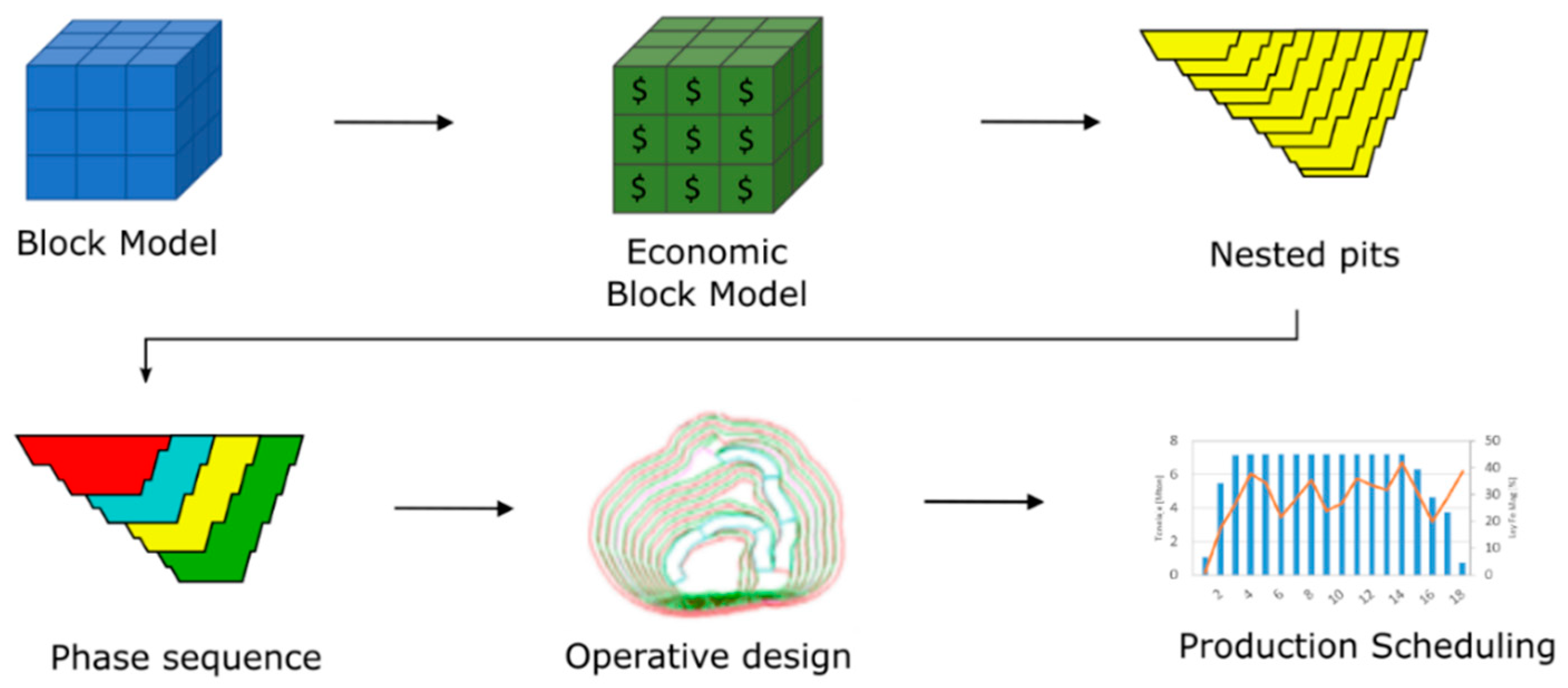
1.1. Mine Planning
1.2. Geometallurgy
1.2.1. Geometallurgical Variables
1.2.2. Metallurgical Recovery
1.2.3. Comminution Performance
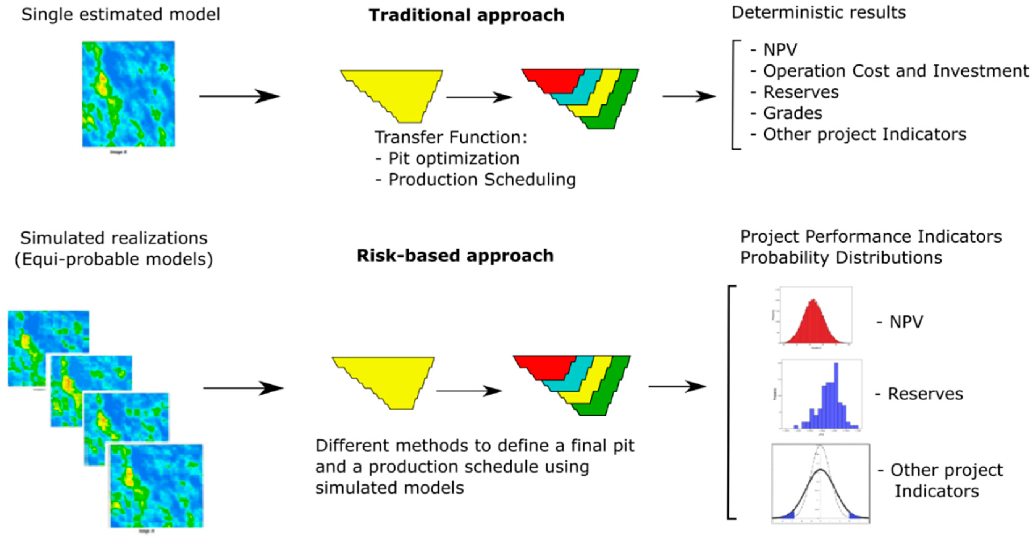
1.3. Modeling the Uncertainty
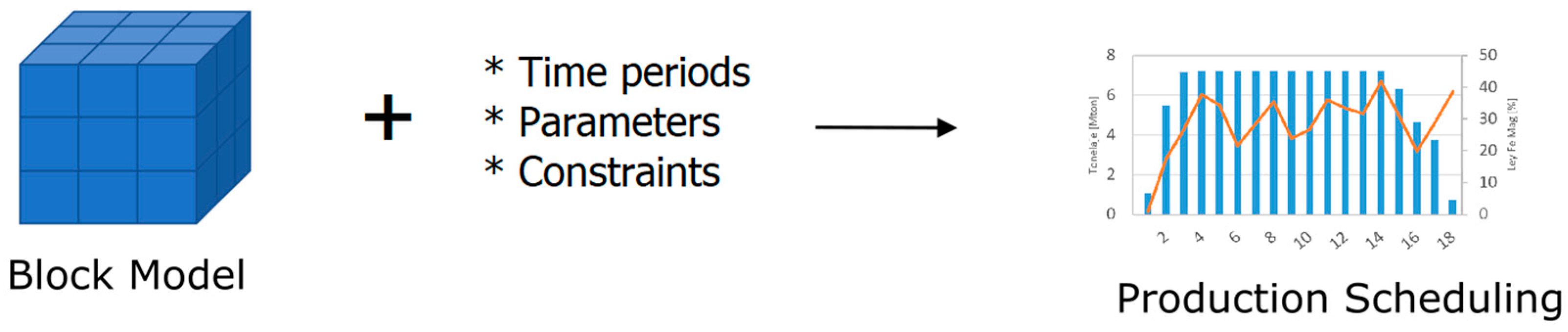
1.4. Background on Direct Block Scheduling
1.5. Contribution of the Research
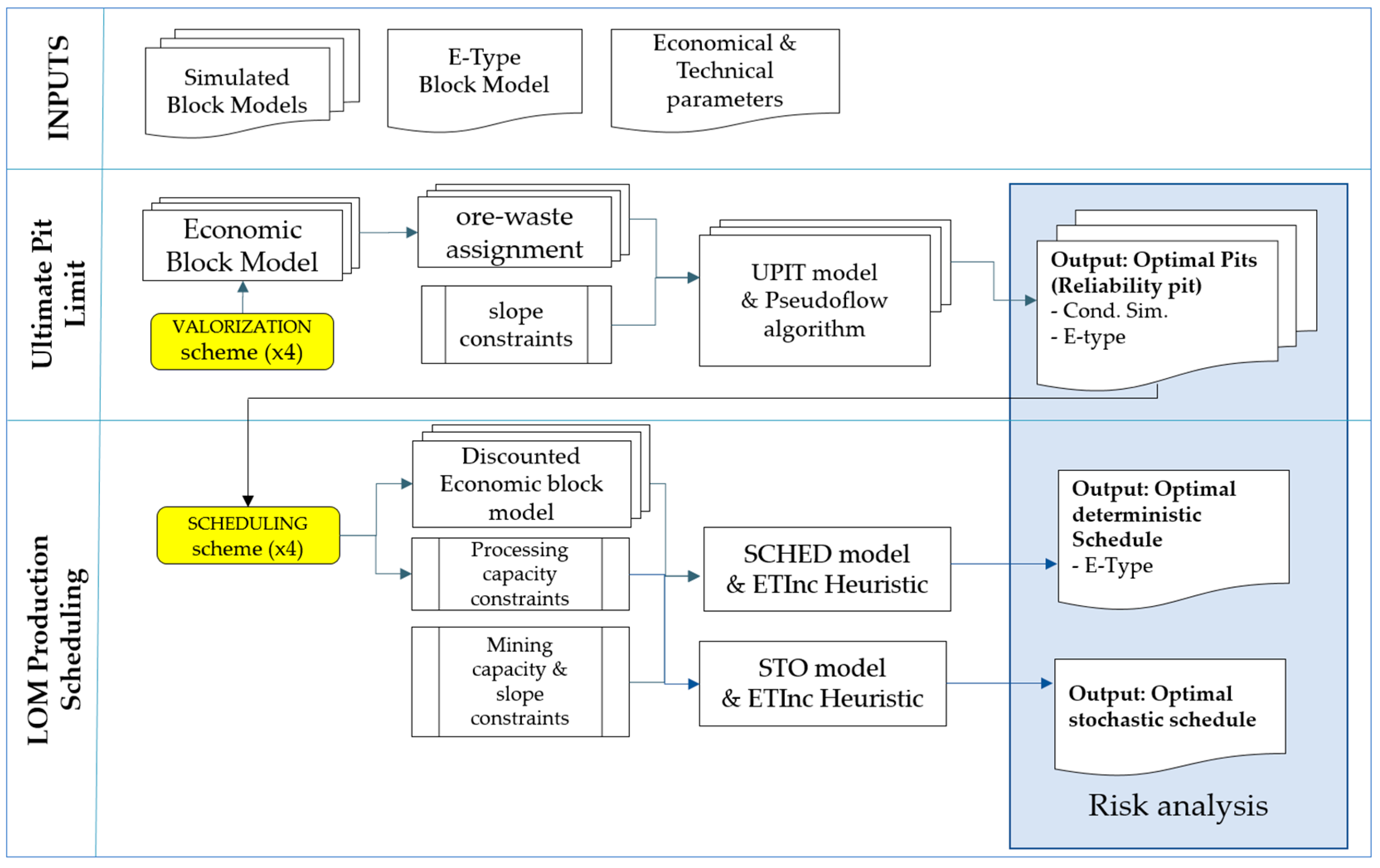
2. Materials and Methods
2.1. Notation
| Scheme 1 | (1) | ||
| Scheme 2 | (2) | ||
| Scheme 3 | (3) | ||
| Scheme 4 | (4) |
2.2. Ultimate Pit Limit
2.3. LOM Production Scheduling
2.3.1. Deterministic Direct Block Scheduling
- Scheduling Scheme 1: the economic block model is constructed according Equation (1), that is, just considering deterministic variables (E-Type models). The minimum and maximum processing capacities are assumed fixed.
| Scheduling Scheme 1 | (14) |
2.3.2. Stochastic Direct Block Scheduling
- Scheduling Scheme 2: the economic block model is constructed according (2), therefore two simulated variables (Cu grade and Mo grade) are considered. Minimum/maximum processing capacities are fixed.
- Scheduling Scheme 3: the economic block model is constructed according (3), therefore three simulated variables (Cu grade, Mo grade and Cu recovery) are considered. As before, minimum/maximum processing capacities are fixed.
- Scheduling Scheme 4: the economic block model is constructed according (4), but processing capacity constraint per period changes. While in the previous cases the maximum processing capacities per period are considered in terms of tonnages, in this case the total available times at the milling plant is considered at a given period as constraint. For this purpose, the milling hours for each block are calculated based on TPH model. Therefore, in this case, the four simulated variables are considered (Cu grade, Mo grade, Cu recovery and TPH).
| Scheduling Scheme 2,3 | (23) |
| Scheduling Scheme 4 | (24) |
3. Case Study and Results
3.1. Case Study
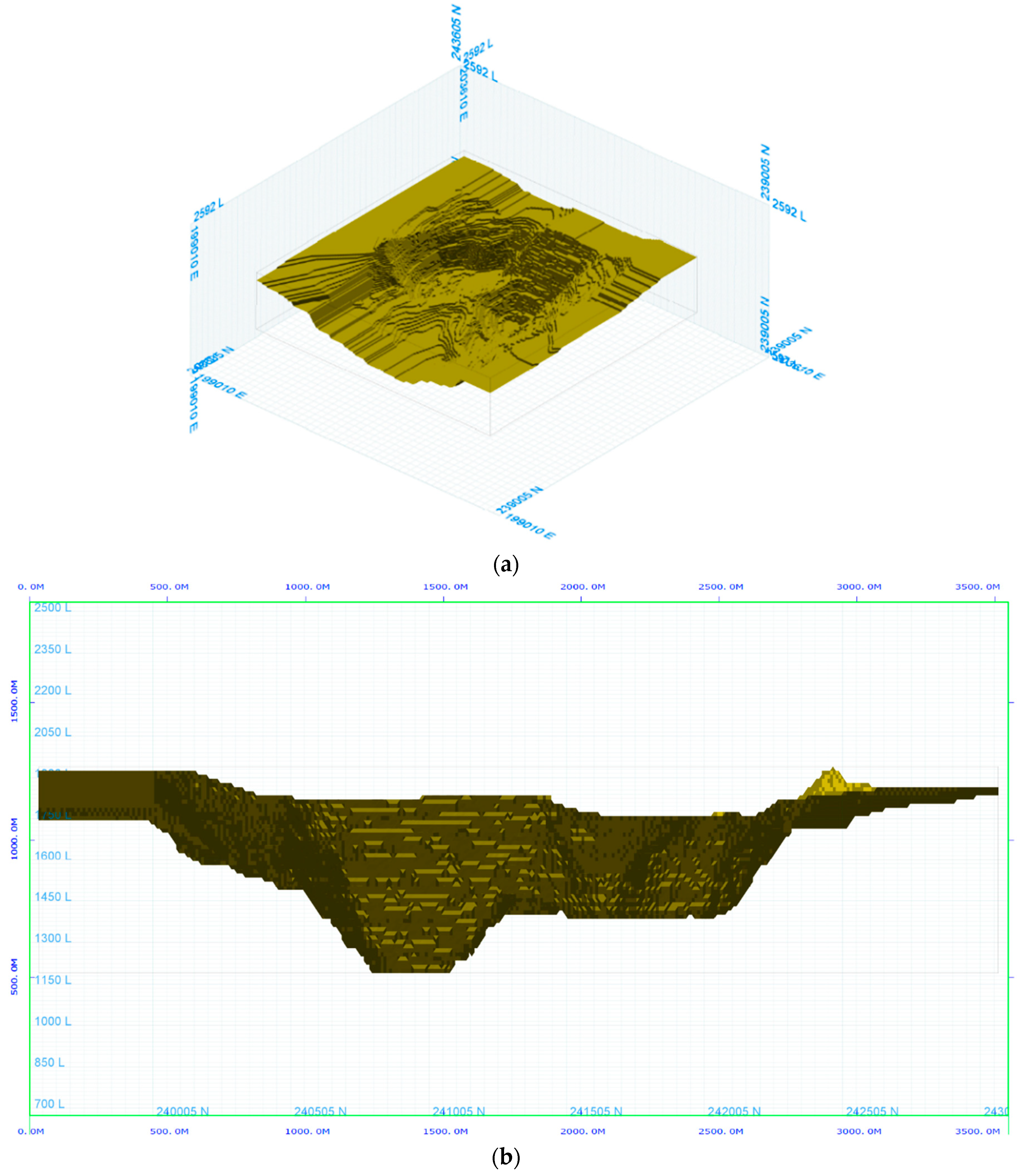
3.1.1. Block Model
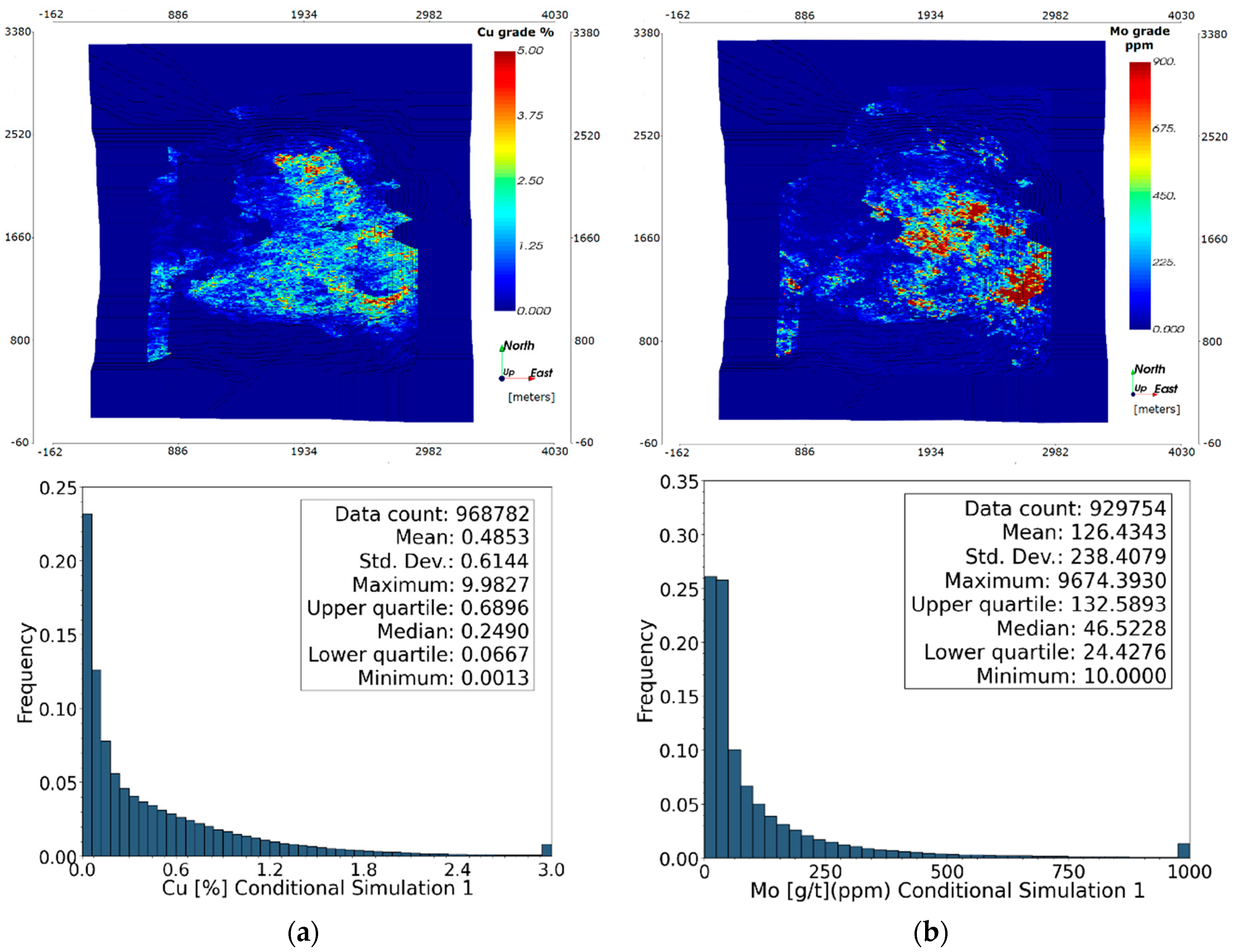
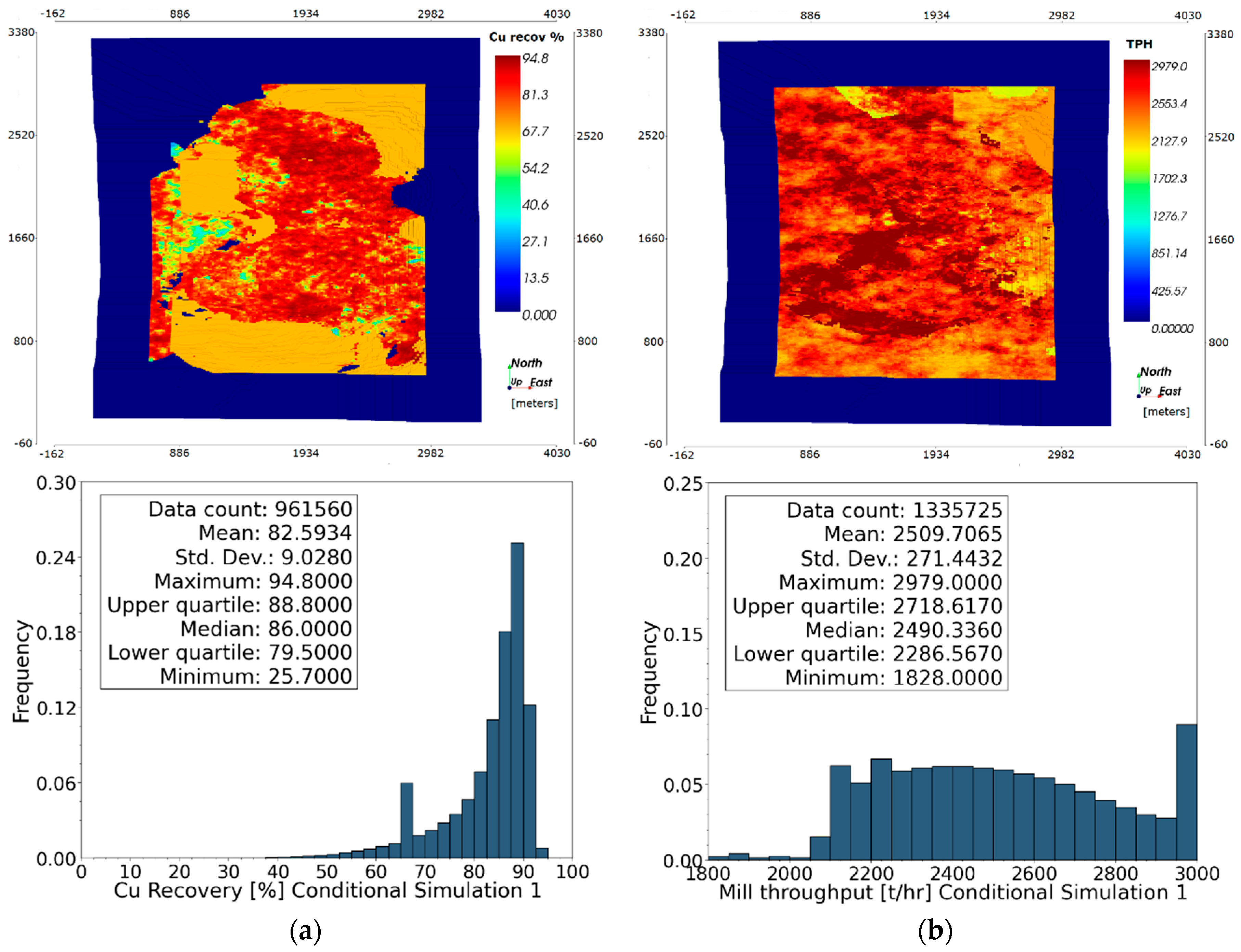
3.1.2. Simulated Geometallurgical Variables
- Grades: Cu (%) and Mo (gr/ton or ppm),
- Cu metallurgical recovery,
- Throughput rate (TPH): this variable predicts the tons per hour that can be processed in the milling circuit and it based on grindability test data (see Section 1.2.3) and the current operational configuration.
3.1.3. Economic Parameters
3.1.4. Technical Parameters
3.2. Results
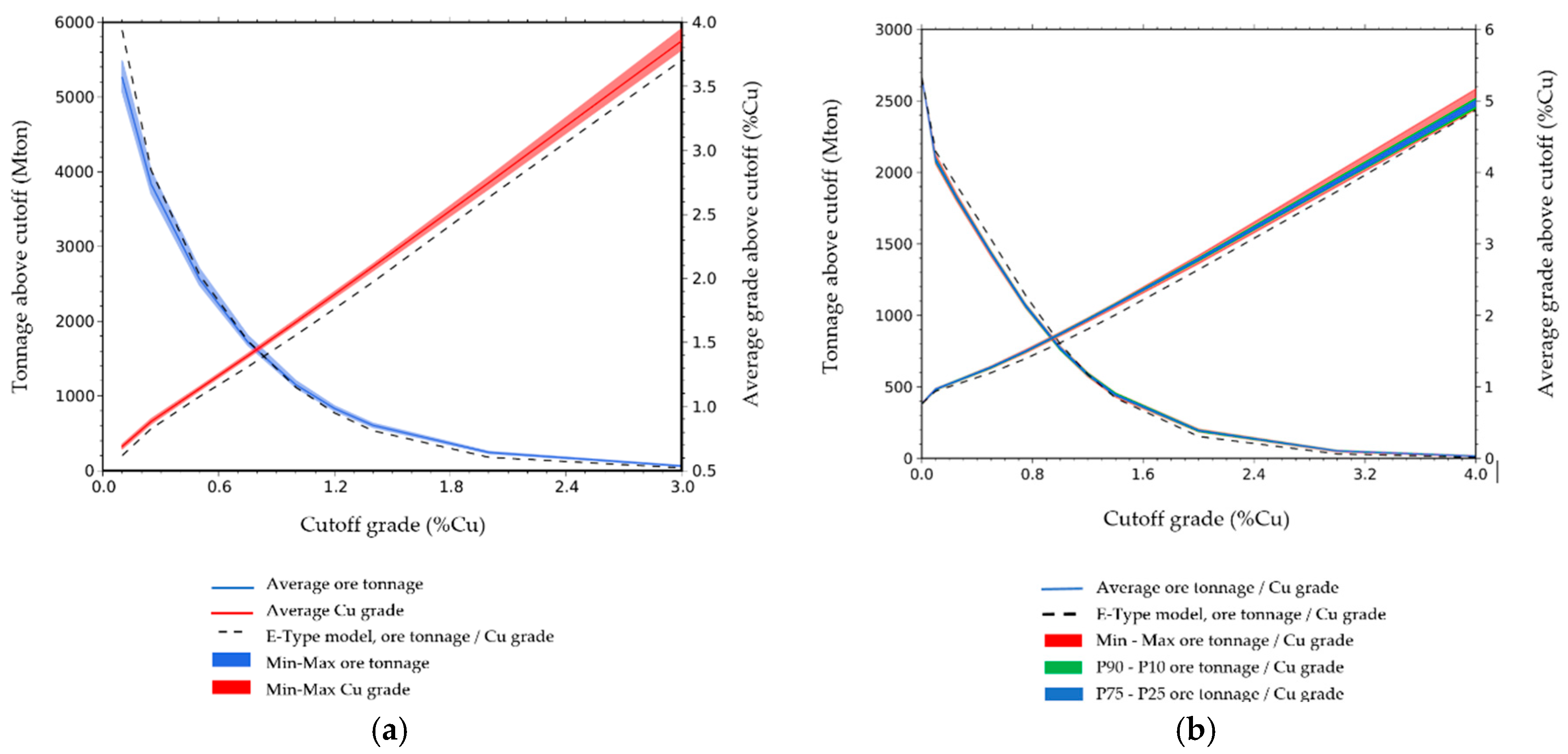
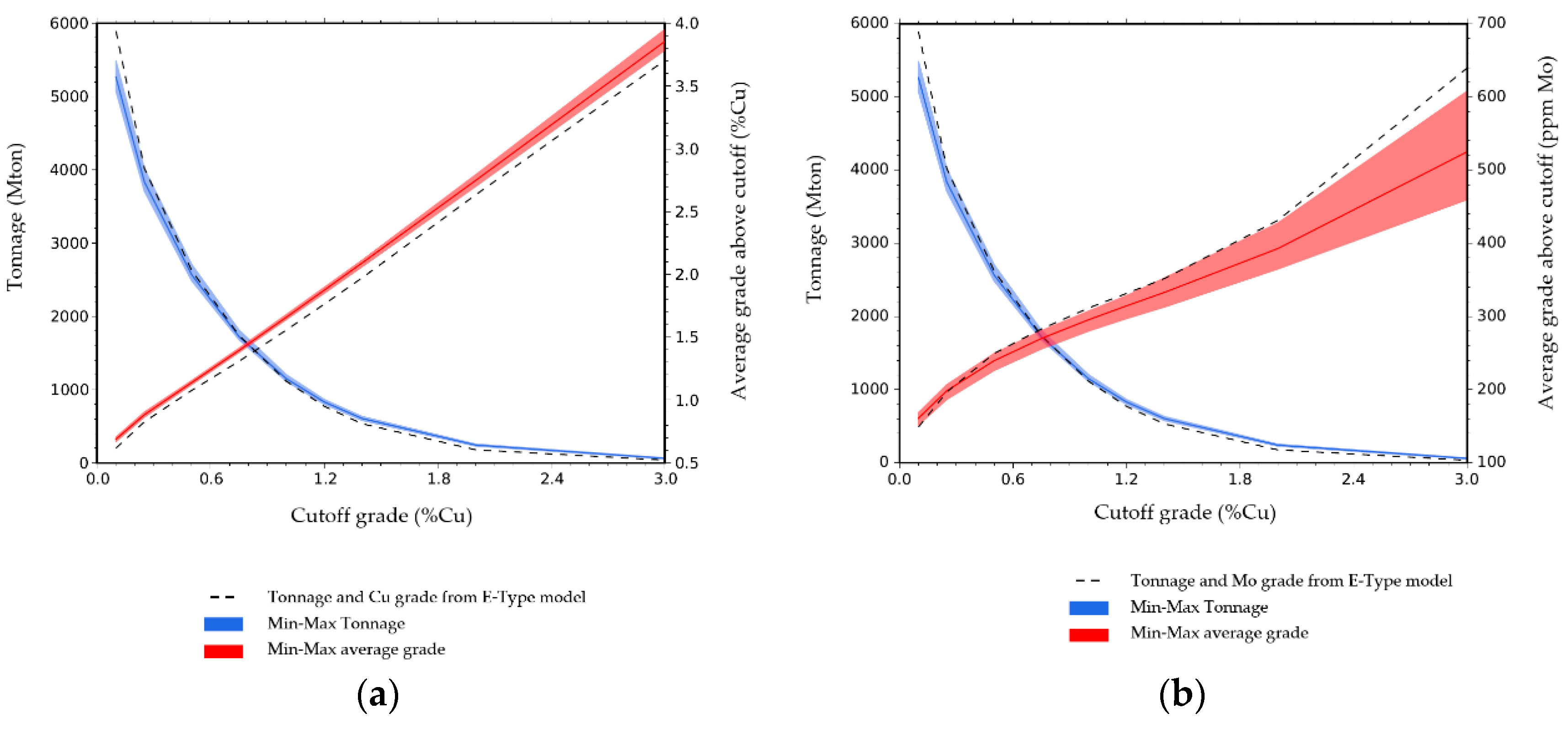
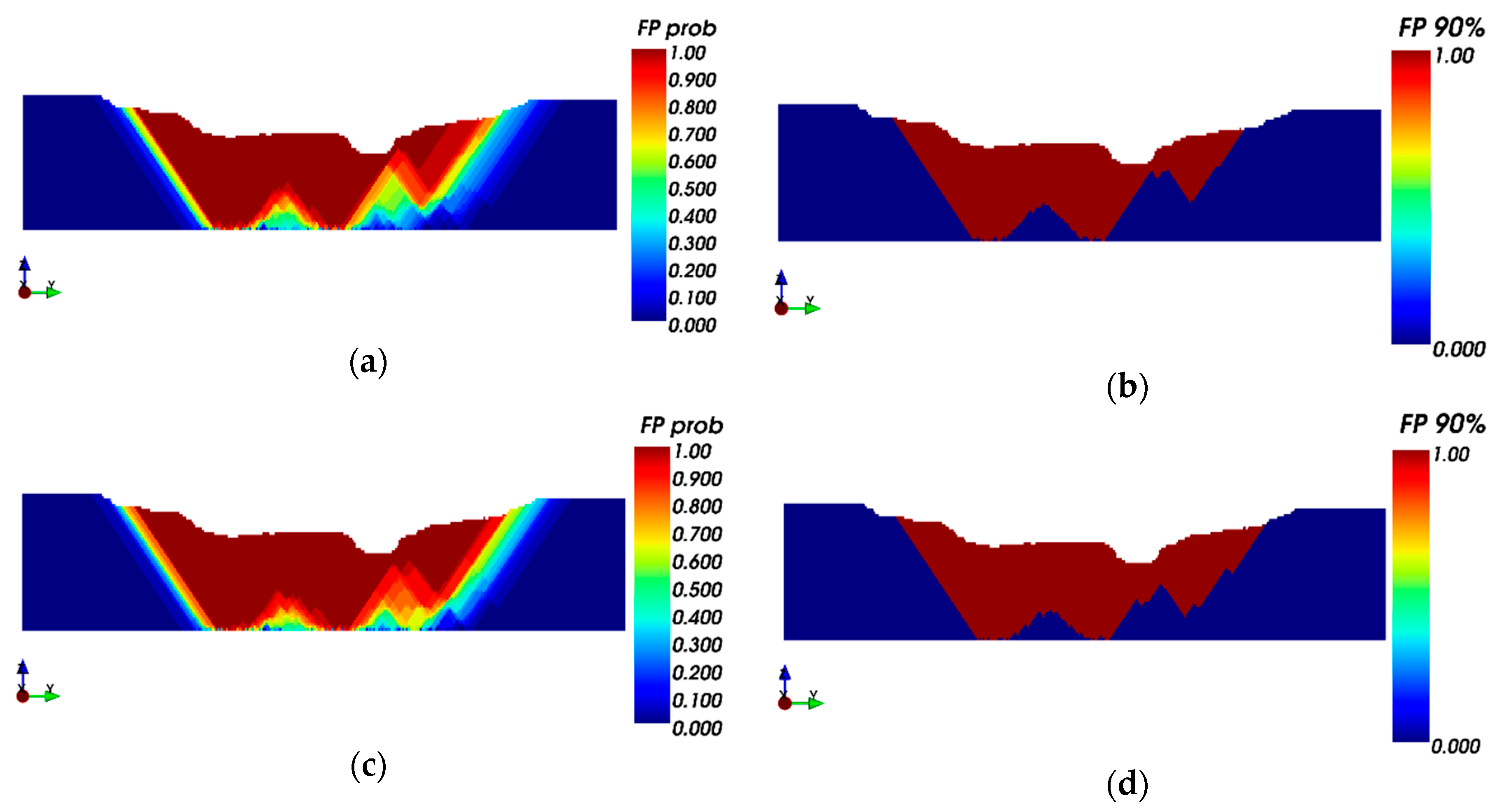
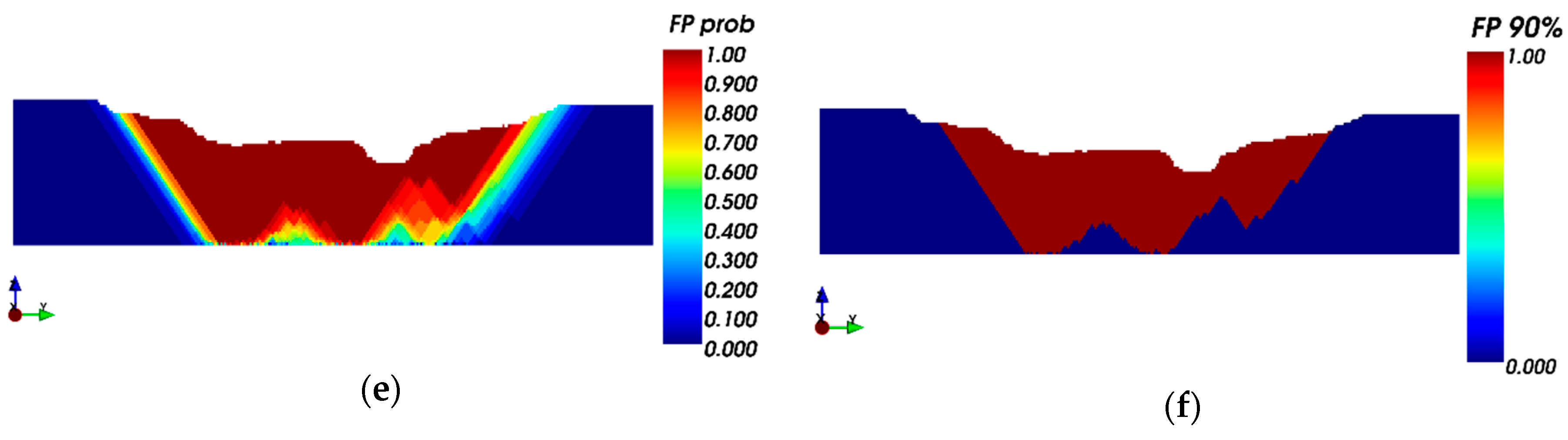
3.2.1. Ultimate Pit Limit: Key Indicators Results and Risk Analysis
Probability Model Results
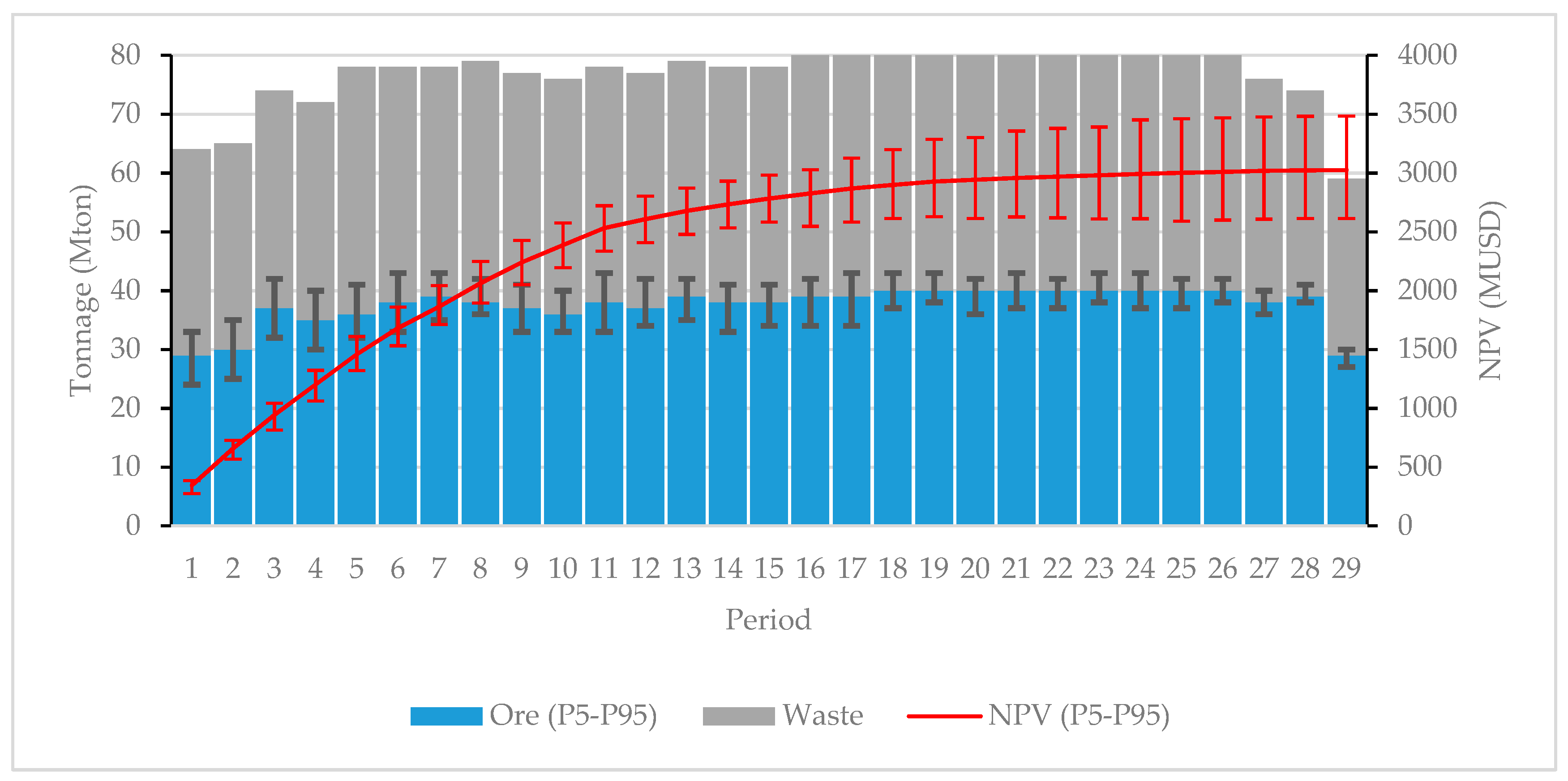
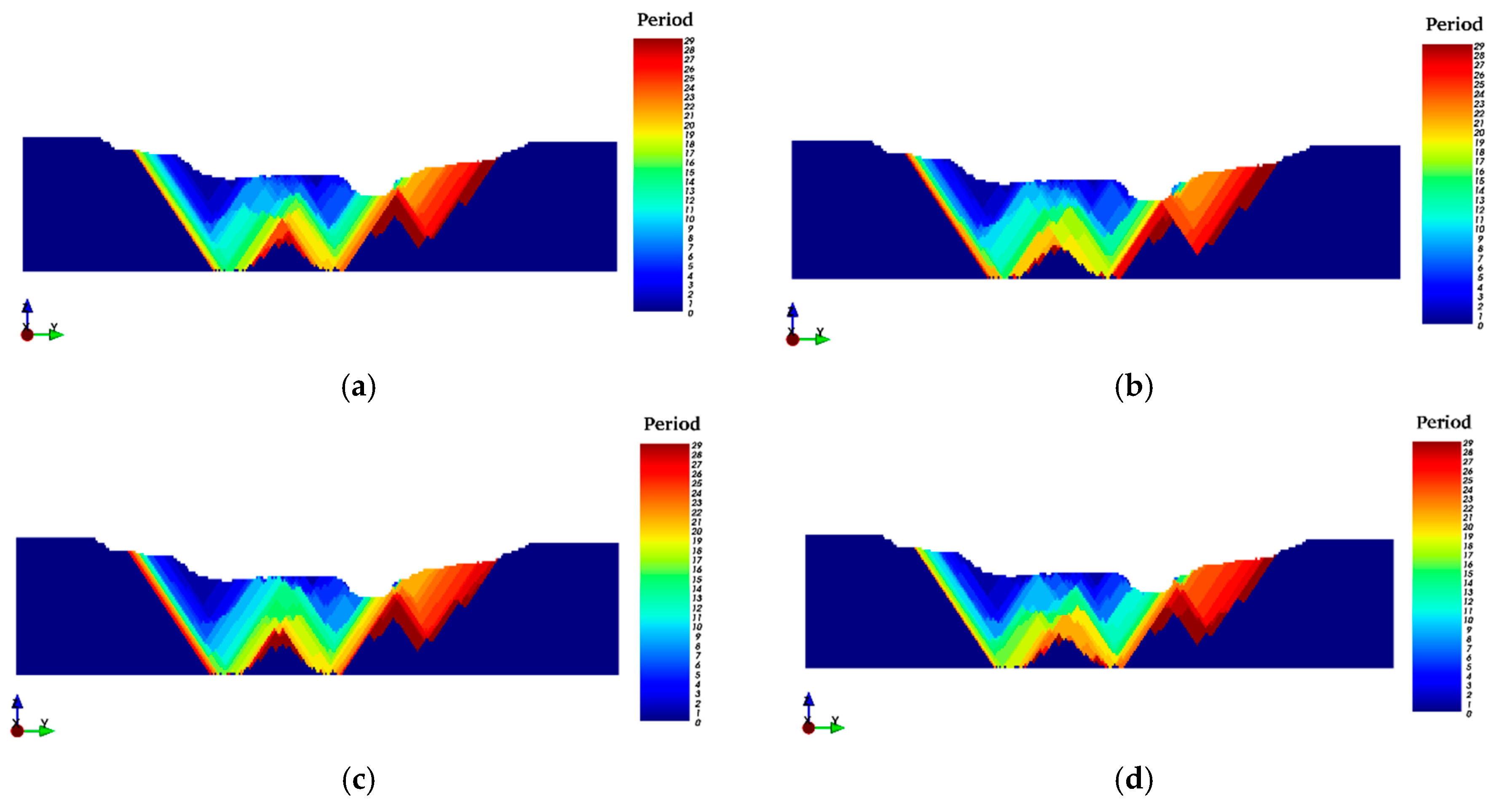
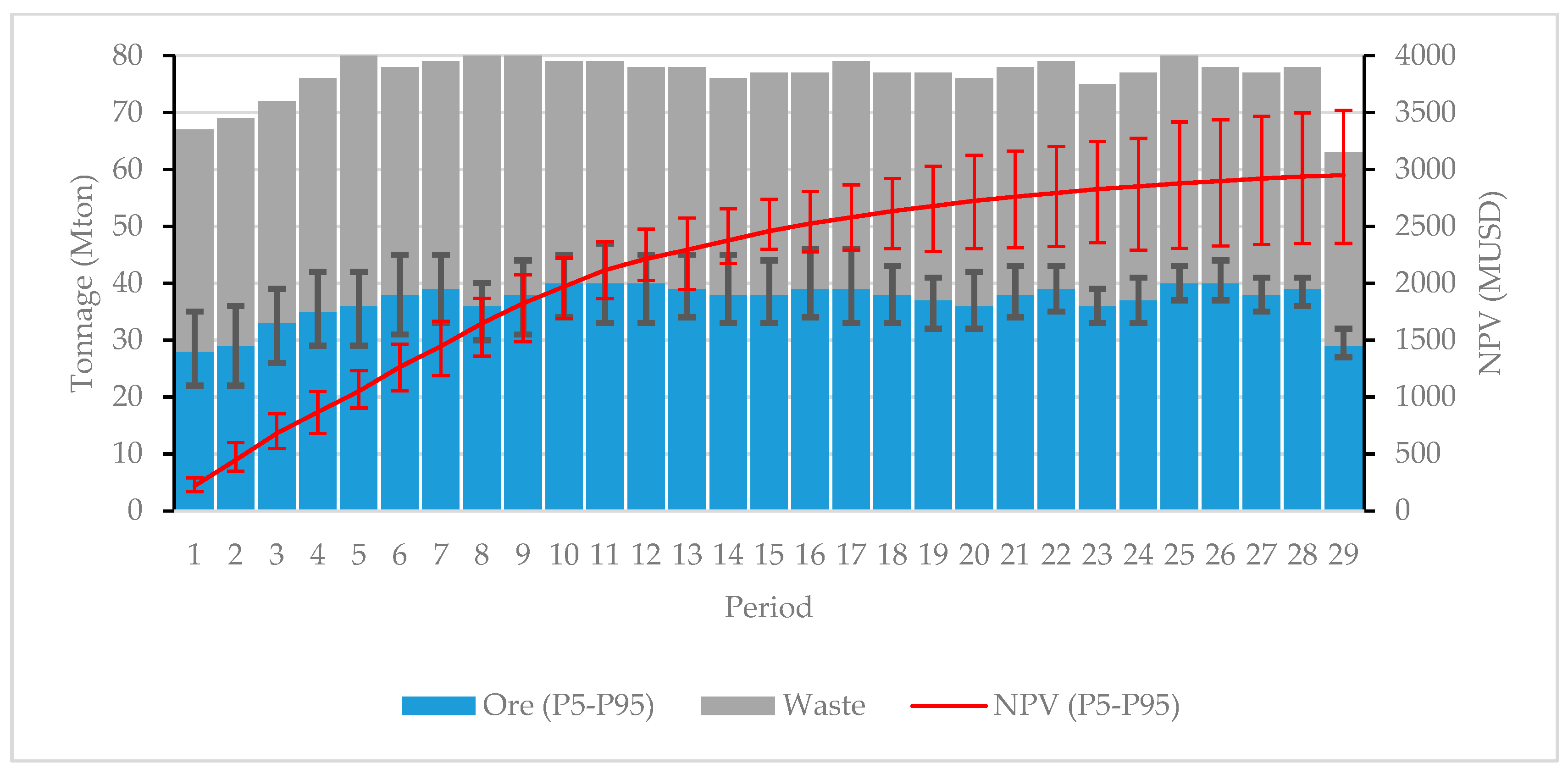
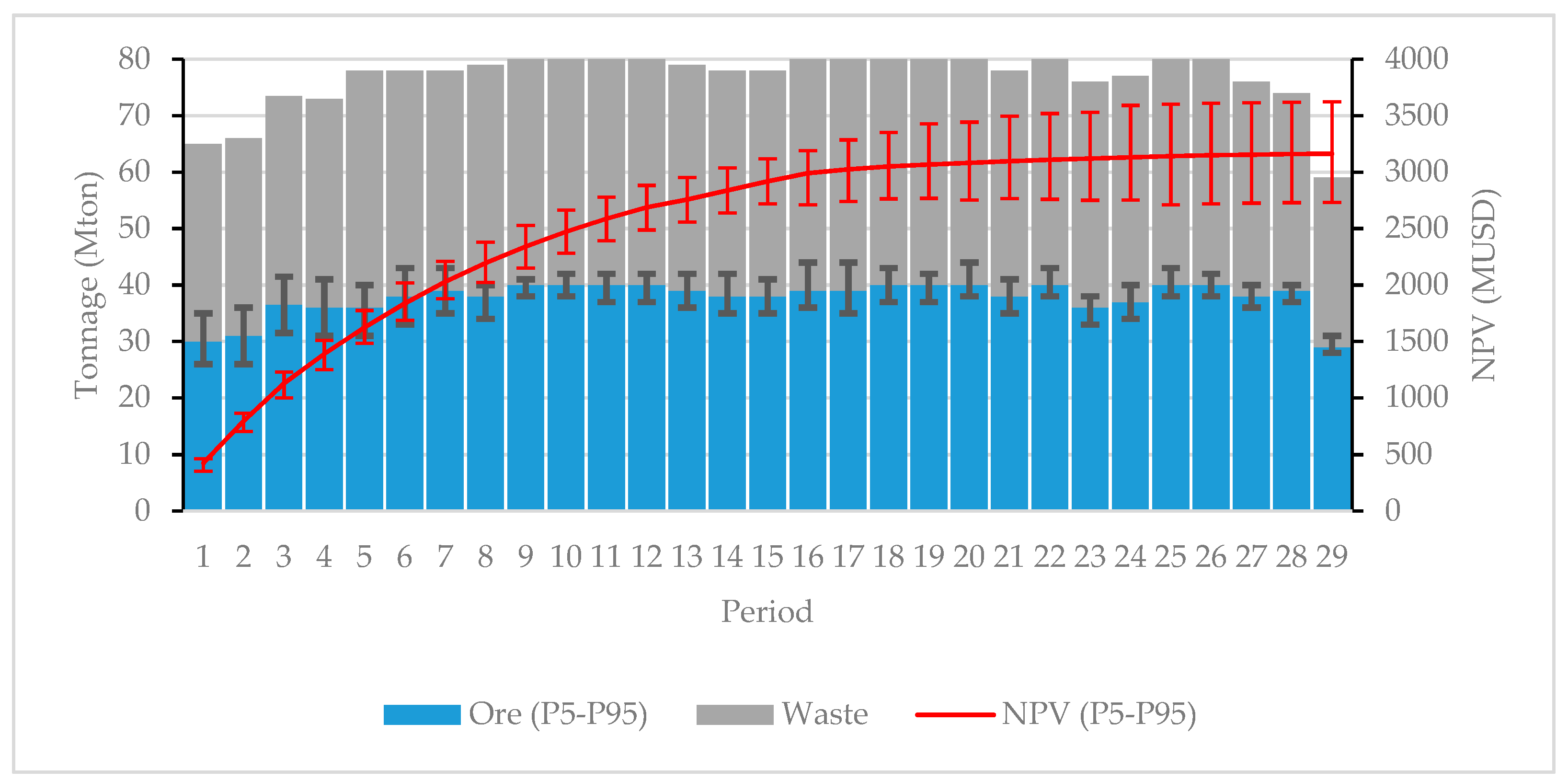
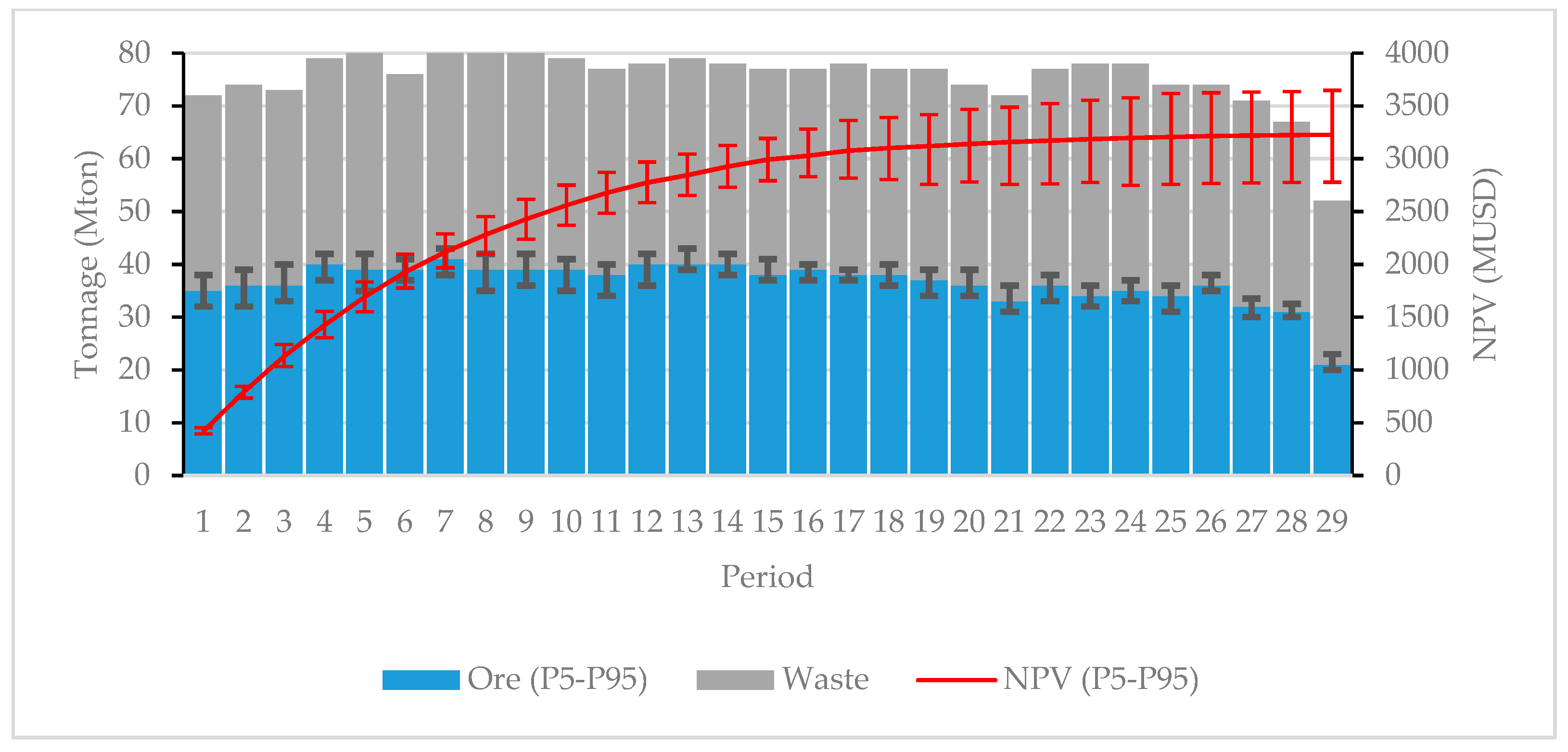
3.2.2. LOM Production Scheduling
4. Discussion
5. Conclusions
- Geological and geometallurgical scenarios are considered in one-run as input to the optimization process,
- the extraction period for each mining block is determined,
- the solution achieves the maximum discounted economic benefit of the mining business,
- the solution achieves the minimum risk of losses due to potential deviations from the production plan,
- the solution satisfies operational constraints, such as slope angles in pit walls and mining capacities.
Author Contributions
Funding
Conflicts of Interest
References
- Chilès, J.P.; Delfiner, P. Geostatistics: Modeling Spatial Uncertainty; John Wiley & Sons: Hoboken, NJ, USA, 2009; ISBN 978-0-470-31783-9. [Google Scholar]
- Lerchs, H.; Grossmann, I.F. Optimum Design of Open-Pit Mines. Tran. Can. Inst. Min. 1965, 58, 17–24. [Google Scholar]
- Meagher, C.; Dimitrakopoulos, R.; Avis, D. Optimized open pit mine design, pushbacks and the gap problem—A review. J. Min. Sci. 2014, 50, 508–526. [Google Scholar] [CrossRef]
- Jélvez, E.; Morales, N.; Askari-Nasab, H. A new model for automated pushback selection. Comput. Oper. Res. 2018. [Google Scholar] [CrossRef]
- Heidari, S.M. Quantification of Geological Uncertainty and Mine Planning Risk Using Metric Spaces. Ph.D. Thesis, University of New South Wales Mining Engineering, Sydney, Australia, March 2015. [Google Scholar]
- Walters, S.G. An overview of new integrated geometallurgical research. In Proceedings of the 9th International Congress for Applied Mineralogy, Brisbane, Australia, 8–10 September 2008; Australasian Institute of Mining and Metallurgy: Carlton, Australia, 2008; pp. 79–82. [Google Scholar]
- Deutsch, C.V. Geostatistical modelling of geometallurgical variables—Problems and solutions. In Proceedings of the 2nd AusIMM International Geometallurgy Conference, GeoMet, Brisbane, Australia, 30 September–2 October 2013; Dominy, S., Ed.; Australasian Institute of Mining and Metallurgy: Carlton, Australia, 2013; pp. 7–16. [Google Scholar]
- Lund, C.; Lamberg, P. Geometallurgy—A tool for better resource efficiency. Eur. Geol. 2014, 37, 39–43. [Google Scholar]
- Dominy, S.C.; O’Connor, L.; Parbhakar-Fox, A.; Glass, H.J.; Purevgerel, S. Geometallurgy—A Route to More Resilient Mine Operations. Minerals 2018, 8, 560. [Google Scholar] [CrossRef]
- Cáceres, A.; Pelley, C.W.; Katsabanis, P.D.; Kelebek, S. Integrating Work Index to Mine Planning at Large Scale Mining Operations. In Proceedings of the 2nd International Conference on Mining Innovation-MININ 2006, Santiago, Chile, 23–26 May 2006; Ortíz, J., Ed.; DIMIN, UChile: Santiago, Chile, 2006; pp. 465–476. [Google Scholar]
- Dunham, S.; Vann, J. Geometallurgy, geostatistics and project value—Does your block model tell you what you need to know? In Proceedings of the Project Evaluation Conference, Melbourne, Australia, 19–20 June 2007; Australasian Institute of Mining and Metallurgy: Carlton, Australia, 2007; pp. 189–196. [Google Scholar]
- Coward, S.; Vann, J.; Dunham, S.; Stewart, M. The primary-response framework for geometallurgical variables. In Proceedings of the 7th International Mining Geology Conference, Perth, Australia, 17–19 August 2009; Dominy, S., Ed.; Australasian Institute of Mining and Metallurgy: Melbourne, Australia, 2009; pp. 109–113. [Google Scholar]
- Contreras, R.E.; Ortíz, J.M.; Bisso, C. Mine planning considering uncertainty in grades and work index. In Proceedings of the 4th International Conference on Mining Innovation-MININ 2010, Santiago, Chile, 23–25 June 2010; Castro, R., Ed.; Gecamin: Santiago, Chile, 2010; pp. 129–136. [Google Scholar]
- Coward, S.; Dowd, P.A.; Vann, J. Value chain modelling to evaluate geometallurgical recovery factors. In Proceedings of the 36th APCOM Conference, Porto Alegre, Brazil, 4–8 November 2013; Costa, J.F., Ed.; Fundação Luiz Englert: Porto Alegre, Brazil, 2013; pp. 288–298. [Google Scholar]
- Coward, S.; Dowd, P.A. Geometallurgical models for the quantification of uncertainty in mining project value chains. In Proceedings of the 37th APCOM Conference, Fairbanks, AK, USA, 23–27 May 2015; Bandopadhyay, S., Ed.; SME: Englewood, CO, USA, 2015; pp. 360–369. [Google Scholar]
- Dowd, P.A.; Xu, C.; Coward, S. Strategic mine planning and design: Some challenges and strategies for addressing them. Min. Technol. 2016, 125, 22–34. [Google Scholar] [CrossRef]
- Kennedy, B.A. Surface Mining, 2nd ed.; SME: Littleton, CO, USA, 1990; ISBN 978-0-87335-102-7. [Google Scholar]
- Sepulveda, E.; Dowd, P.A.; Xu, C.; Addo, E. Multivariate Modelling of Geometallurgical Variables by Projection Pursuit. Math Geosci. 2017, 49, 121–143. [Google Scholar] [CrossRef]
- Monkhouse, P.H.L.; Yeates, G.A. Beyond Naïve Optimisation. In Advances in Applied Strategic Mine Planning; Springer: Cham, Switzerland, 2018; pp. 3–18. ISBN 978-3-319-69319-4. [Google Scholar]
- Carrasco, P.; Chilès, J.-P.; Séguret, S.A. Additivity, metallurgical recovery, and grade. In Proceedings of the 8th International Geostatistics Congress, Santiago, Chile, 1–5 December 2008; Ortíz, J., Ed.; GECAMIN: Santiago, Chile, 2008. [Google Scholar]
- Mwanga, A.; Rosenkranz, J.; Lamberg, P. Testing of Ore Comminution Behavior in the Geometallurgical Context—A Review. Minerals 2015, 5, 276–297. [Google Scholar] [CrossRef]
- Yap, A.; Saconi, F.; Nehring, M.; Arteaga, F.; Pinto, P.; Asad, M.W.A.; Ozhigin, S.; Ozhigina, S.; Mozer, D.; Nagibin, A.; et al. Exploiting the metallurgical throughput–recovery relationship to optimise resource value as part of the production scheduling process. Miner. Eng. 2013, 53, 74–83. [Google Scholar] [CrossRef]
- Dowd, P.A. Risk assessment in reserve estimation and open-pit planning. Trans. Inst. Min. Metall. Sect. A Min. Ind. 1994, 103, A148–A154. [Google Scholar]
- Smith, M.; Dimitrakopoulos, R. The influence of deposit uncertainty on mine production scheduling. Interface J. Surf. Min. Reclam. Environ. 1999, 13, 173–178. [Google Scholar] [CrossRef]
- Journel, A.G.; Huijbregts, C. Mining Geostatistics; Academic Press: Cambridge, MA, USA, 1978; ISBN 978-0-12-391050-9. [Google Scholar]
- Deutsch, J.L.; Palmer, K.; Deutsch, C.V.; Szymanski, J.; Etsell, T.H. Spatial Modeling of Geometallurgical Properties: Techniques and a Case Study. Nat. Resour. Res. 2016, 25, 161–181. [Google Scholar] [CrossRef]
- Dimitrakopoulos, R. Advances in Applied Strategic Mine Planning; Springer: Cham, Switzerland, 2018; ISBN 978-3-319-69320-0. [Google Scholar]
- Godoy, M. The Efficient Management of Geological Risk in Long-Term Production Scheduling of Open Pit Mines. Ph.D. Thesis, University of Queensland, Brisbane, Australia, December 2003. [Google Scholar]
- Leite, A.; Dimitrakopoulos, R. Stochastic optimisation model for open pit mine planning: Application and risk analysis at copper deposit. Min. Technol. 2007, 116, 109–118. [Google Scholar] [CrossRef]
- Consuegra, F.R.A.; Dimitrakopoulos, R. Stochastic mine design optimisation based on simulated annealing: pit limits, production schedules, multiple orebody scenarios and sensitivity analysis. Min. Technol. 2009, 118, 79–90. [Google Scholar] [CrossRef]
- Vielma, J.P.; Espinoza, D.; Moreno, E. Risk control in ultimate pits using conditional simulations. In Proceedings of the 34th APCOM Conference, Vancouver, BC, Canada, 6–9 October 2009; CIMM: Vancouver, BC, Canada, 2009; pp. 107–114. [Google Scholar]
- Ramazan, S.; Dimitrakopoulos, R. Stochastic Optimisation of Long-Term Production Scheduling for Open Pit Mines with a New Integer Programming Formulation. In Advances in Applied Strategic Mine Planning; Springer: Cham, Switzerland, 2018; pp. 139–153. ISBN 978-3-319-69319-4. [Google Scholar]
- Johnson, T.B. Optimum Open-Pit Mine Production Scheduling. Ph.D. Thesis, University of California, Berkeley, CA, USA, May 1968. [Google Scholar]
- Morales, N.; Jélvez, E.; Nancel-Penard, P.; Marinho, A.; Guimaräes, O. A comparison of conventional and direct block scheduling methods for open pit mine production scheduling. In Proceedings of the 37th APCOM Conference, Fairbanks, AK, USA, 23–27 May 2015; Bandopadhyay, S., Ed.; SME: Englewood, CO, USA, 2015; pp. 1040–1051. [Google Scholar]
- Caccetta, L.; Hill, S.P. An application of branch and cut to open pit mine scheduling. J. Glob. Optim. 2003, 27, 349–365. [Google Scholar] [CrossRef]
- Chicoisne, R.; Espinoza, D.; Goycoolea, M.; Moreno, E.; Rubio, E. A New Algorithm for the Open-Pit Mine Production Scheduling Problem. Oper. Res. 2012, 60, 517–528. [Google Scholar] [CrossRef]
- Jélvez, E.; Morales, N.; Nancel-Penard, P.; Peypouquet, J.; Reyes, P. Aggregation heuristic for the open-pit block scheduling problem. Eur. J. Oper. Res. 2016, 249, 1169–1177. [Google Scholar] [CrossRef]
- Dimitrakopoulos, R. Stochastic optimization for strategic mine planning: A decade of developments. J. Min. Sci. 2011, 47, 138–150. [Google Scholar] [CrossRef]
- Koushavand, B.; Askari-Nasab, H.; Deutsch, C.V. A linear programming model for long-term mine planning in the presence of grade uncertainty and a stockpile. Int. J. Min. Sci. Technol. 2014, 24, 451–459. [Google Scholar] [CrossRef]
- Jélvez, E. Multistep Methodology for the Long-Term Open-Pit Mine Production Planning Problem under Geological Uncertainty. Ph.D. Thesis, Department of Mining Engineering, Universidad de Chile, Santiago, Chile, April 2017. [Google Scholar]
- Dimitrakopoulos, R.; Farrelly, C.T.; Godoy, M. Moving forward from traditional optimization: Grade uncertainty and risk effects in open-pit design. Min. Technol. 2002, 111, 82–88. [Google Scholar] [CrossRef]
- Godoy, M. A Risk Analysis Based Framework for Strategic Mine Planning and Design—Method and Application. In Advances in Applied Strategic Mine Planning; Springer: Cham, Switzerland, 2018; pp. 75–90. ISBN 978-3-319-69319-4. [Google Scholar]
- Newman, A.M.; Rubio, E.; Caro, R.; Weintraub, A.; Eurek, K. A Review of Operations Research in Mine Planning. Interfaces 2010, 40, 222–245. [Google Scholar] [CrossRef]
- Espinoza, D.; Goycoolea, M.; Moreno, E.; Newman, A. MineLib: A library of open pit mining problems. Ann. Oper. Res. 2013, 206, 93–114. [Google Scholar] [CrossRef]
- Hochbaum, D.S.; Chen, A. Performance Analysis and Best Implementations of Old and New Algorithms for the Open-Pit Mining Problem. Oper. Res. 2000, 48, 894–914. [Google Scholar] [CrossRef]
- Hochbaum, D.S. The Pseudoflow Algorithm: A New Algorithm for the Maximum-Flow Problem. Oper. Res. 2008, 56, 992–1009. [Google Scholar] [CrossRef]
- Chandran, B.G.; Hochbaum, D.S. A Computational Study of the Pseudoflow and Push-Relabel Algorithms for the Maximum Flow Problem. Oper. Res. 2009, 57, 358–376. [Google Scholar] [CrossRef]
- Hochbaum, D.S.; Orlin, J.B. Simplifications and speedups of the pseudoflow algorithm. Networks 2013, 61, 40–57. [Google Scholar] [CrossRef]
- Jélvez, E.; Morales, N.; Nancel-Penard, P. Open-pit mine production scheduling: Improvements to MineLib library problems. In Proceedings of the 27th International Symposium on Mine Planning and Equipment Selection–MPES 2018, Santiago, Chile, 20–22 November 2018; Widzyk-Capehart, E., Hekmat, A., Singhal, R., Eds.; Springer: Cham, Switzerland, 2018. Chapter 18. pp. 223–232, ISBN 978-3-319-99220-4. [Google Scholar] [CrossRef]
- Whittle, D.; Bozorgebrahimi, A. Hybrid Pits—Linking Conditional Simulation and Lerchs-Grossmann Through Set Theory. In Proceedings of the Symposium on Orebody Modelling and Strategic Mine Planning, Perth, Australia, 22–24 November 2004; Dimitrakopoulos, R., Ed.; Australasian Institute of Mining and Metallurgy: Carlton, Australia, 2004; pp. 37–42. [Google Scholar]
- Lamghari, A.; Dimitrakopoulos, R. Progressive hedging applied as a metaheuristic to schedule production in open-pit mines accounting for reserve uncertainty. Eur. J. Oper. Res. 2016, 253, 843–855. [Google Scholar] [CrossRef]
- Lamghari, A.; Dimitrakopoulos, R. Network-flow based algorithms for scheduling production in multi-processor open-pit mines accounting for metal uncertainty. Eur. J. Oper. Res. 2016, 250, 273–290. [Google Scholar] [CrossRef]
- Lamghari, A.; Dimitrakopoulos, R. Hyper-heuristic approaches for strategic mine planning under uncertainty. Comput. Oper. Res. 2018. [Google Scholar] [CrossRef]


| Symbol | Unit | Parameter |
|---|---|---|
| USD/lb | Cu price | |
| USD/lb | Mo price | |
| USD/lb | Cu selling cost | |
| USD/lb | Mo selling cost | |
| USD/ton | Mining cost | |
| USD/ton | Processing cost (main) | |
| USD/ton | Mo processing cost |
| Scheme | Cu Grade | Mo Grade | Cu Recovery | TPH |
|---|---|---|---|---|
| 1 | ✕ | ✕ | ✕ | ✕ |
| 2 | ✓ | ✓ | ✕ | ✕ |
| 3 | ✓ | ✓ | ✓ | ✕ |
| 4 | ✓ | ✓ | ✓ | ✓ |
| Symbol | Unit | Parameter | Value |
|---|---|---|---|
| USD/lb | Cu price | 1.80 | |
| USD/lb | Mo price | 6.00 | |
| USD/lb | Cu selling cost | 0.40 | |
| USD/lb | Mo selling cost | 1.72 | |
| USD/ton | Mining cost | 3.79 | |
| USD/ton | Processing cost (main) | 11.35 | |
| USD/ton | Mo processing cost | 15.58 | |
| (*) | USD/ton | Unitary shortage cost | 30.00 |
| (*) | USD/ton | Unitary surplus cost | 30.00 |
| (**) | USD/h | Unitary shortage cost | 70,000.00 |
| (**) | USD/h | Unitary surplus cost | 70,000.00 |
| Symbol | Unit | Parameter | Value |
|---|---|---|---|
| - | Mo metallurgical recovery | 0.55 | |
| hr/block | Average processing time | 3.18 | |
| degree | Overall slope angle | 42.00 | |
| - | Height (number of upper benches) | 3.00 | |
| Mton | Lower bound mining cap. | 0.00 | |
| Mton | Upper bound mining cap. | 80.00 | |
| (*) | Mton | Lower bound process. cap. | 25.00 |
| (*) | Mton | Upper bound process. cap. | 40.00 |
| (**) | hour | Lower bound process. cap. | 10,000.00 |
| (**) | hour | Upper bound process. cap. | 15,710.00 |
| |T| | year | Planning horizon | 30.00 |
| - | Discount rate | 0.10 |
| Scheme | Undiscounted Value (MUSD) | Rock (Mton) | Ore (Mton) | Cu Metal (Mton) | Mo Metal (Kton) | |||||
|---|---|---|---|---|---|---|---|---|---|---|
| Avg | CV% | Avg | CV% | Avg | CV% | Avg | CV% | Avg | CV% | |
| 1 | 9453 | - | 3071 | - | 1433 | - | 17.5 | - | 388.1 | - |
| 2 | 10,528 | 2.5 | 3372 | 4.1 | 1602 | 2.9 | 18.5 | 1.9 | 471.6 | 3.2 |
| 3 | 10,725 | 3.1 | 3558 | 3.7 | 1682 | 2.4 | 18.9 | 2.5 | 467.2 | 3.8 |
| 4 | 10,472 | 2.1 | 2972 | 3.2 | 1572 | 3.1 | 17.9 | 2.2 | 417.6 | 3.5 |
| Minimum Probability | Scheme 2 | Scheme 3 | Scheme 4 | ||||||
|---|---|---|---|---|---|---|---|---|---|
| Value | Ore | Rock | Value | Ore | Rock | Value | Ore | Rock | |
| (MUSD) | (Mton) | (Mton) | (MUSD) | (Mton) | (Mton) | (MUSD) | (Mton) | (Mton) | |
| 1.0 | 9062 | 1120 | 2320 | 9310 | 1184 | 2492 | 8633 | 988 | 2125 |
| 0.9 | 9134 | 1199 | 2417 | 9422 | 1233 | 2509 | 8708 | 1005 | 2298 |
| 0.8 | 9161 | 1274 | 2721 | 9501 | 1311 | 2718 | 8638 | 1072 | 2407 |
| 0.7 | 9241 | 1295 | 2882 | 9638 | 1375 | 2925 | 8715 | 1163 | 2539 |
| 0.6 | 9395 | 1342 | 2955 | 9793 | 1432 | 3046 | 8865 | 1203 | 2626 |
| 0.5 | 9462 | 1473 | 3086 | 9941 | 1555 | 3173 | 8972 | 1298 | 2710 |
| Scheduling Scheme | Expected NPV | Relative Variation | Expected CDDC | Relative Variation |
|---|---|---|---|---|
| (MUSD) | CDDC % | (MUSD) | CDDC % | |
| 1 | 2949.3 | - | 891.7 | - |
| 2 | 3024.4 | +2.5 | 396.5 | −55.5 |
| 3 | 3162.2 | +7.2 | 389.8 | −56.3 |
| 4 | 3227.3 | +9.4 | 280.4 | −68.6 |
© 2019 by the authors. Licensee MDPI, Basel, Switzerland. This article is an open access article distributed under the terms and conditions of the Creative Commons Attribution (CC BY) license (http://creativecommons.org/licenses/by/4.0/).
Share and Cite
Morales, N.; Seguel, S.; Cáceres, A.; Jélvez, E.; Alarcón, M. Incorporation of Geometallurgical Attributes and Geological Uncertainty into Long-Term Open-Pit Mine Planning. Minerals 2019, 9, 108. https://doi.org/10.3390/min9020108
Morales N, Seguel S, Cáceres A, Jélvez E, Alarcón M. Incorporation of Geometallurgical Attributes and Geological Uncertainty into Long-Term Open-Pit Mine Planning. Minerals. 2019; 9(2):108. https://doi.org/10.3390/min9020108
Chicago/Turabian StyleMorales, Nelson, Sebastián Seguel, Alejandro Cáceres, Enrique Jélvez, and Maximiliano Alarcón. 2019. "Incorporation of Geometallurgical Attributes and Geological Uncertainty into Long-Term Open-Pit Mine Planning" Minerals 9, no. 2: 108. https://doi.org/10.3390/min9020108
APA StyleMorales, N., Seguel, S., Cáceres, A., Jélvez, E., & Alarcón, M. (2019). Incorporation of Geometallurgical Attributes and Geological Uncertainty into Long-Term Open-Pit Mine Planning. Minerals, 9(2), 108. https://doi.org/10.3390/min9020108