1. Introduction
It has long been recognized that the material flux from a mineral surface during dissolution is not homogeneous. Experimentally and analytically, fundamental information about the evolution of reacting surface topographies and their heterogeneity have been gained by using surface-sensitive techniques such as atomic force microscopy, interferometry microscopy, or spectroscopy techniques (e.g., [
1,
2,
3]). Measured reaction rates in laboratory experiments differ significantly under otherwise identical chemical conditions, often up to two to three orders of magnitude (e.g., [
4,
5]), indicating intrinsic differences in crystal surface reactivity [
6]. As yet, a consistent theoretical model based on a purely mechanistic understanding of the heterogeneous distribution of surface reactivity is unavailable, despite its critical importance in understanding processes of, e.g., mineral conversion [
7] or the pore evolution in geological structures [
8]. Consequently, surface rate maps are used to analyze the spatial heterogeneity of crystal surface reactions (e.g., [
9]). Their analysis in the frequency domain by using rate spectra shows the overall rate range and identifies important rate modes that reflect the existence of multiple, concurrent reaction mechanisms [
10,
11]. Mechanistically, crystal defects such as screw dislocations have been identified as the critical factor that constrains the surface evolution during dissolution reactions. After the opening of the hollow cores of defect structures, the subsequent growth of etch pits is dictated by the movement of step waves that ultimately results in complex surface topographies [
12].
Kinetic Monte Carlo simulation techniques have been used to analyze crystal surface reaction kinetics and topography (e.g., [
13,
14,
15]). The analysis of kMC simulation results using the rate spectra concept towards an improved predictability of surface kinetics is promising [
11]. However, the system size of kMC simulations is partly limited by the time required for detailed calculations at each reaction step. In order to overcome this restriction, we explored additional mathematical methods for the simulation of crystal surface evolution during reactions.
The crystal surface morphology is a result of the surface reactivity pattern. Thus, a numerical simulation method capable of predicting the evolution of crystal surface with improved efficiency compared to classical kMC techniques would allow the prediction of surface reaction rates of larger systems. Here, we explore
Voronoi distance maps as a simulation technique for the numerical analysis of reacting crystal surfaces (e.g., [
16]). Using such maps, we evaluate the evolution of kinetic parameters such as the material flux from the surface, the distribution and density of kink sites and ledge sites, as well as the topography and roughness of the crystal surface. We further analyze the correlation of
Voronoi cell parameters such as the metrical distance with crystal surface parameters, e.g., the surface height parameters, calculated using kMC techniques.
The mathematical concept of
Voronoi diagrams aims at partitioning the space into space-filling polyhedrons, based on an assemblage of generating points [
17,
18,
19]. The resulting
Voronoi cells are the regions of minimum distance to those points. This concept was originally derived for the Euclidean distance in three-dimensional space, but is not limited to it. Early crystallographic applications include the analysis of crystal domains arising from regularly distributed sites, leading to an analysis of crystal structure based on the identification of types of space-filling polyhedra [
20]. Another crystallographic concept using the
Voronoi diagrams is the so-called Wigner–Seitz cell. Here, the lattice points of a crystal structure serve as the generating points of such primitive cells [
21]. In reciprocal space, this type of cell is called Brillouin zone [
22] and has many important applications, such as determining the band-structure of a material and determining whether it is an insulator, semiconductor, or conductor. While those
Voronoi cell applications are based on a regular distribution of generating points and Euclidean distance, more recent applications have focused on irregular spacing of generating points and different metrics are used as distance. For example, Kobayashi and Sugihara [
23] used multiplicatively weighted crystal growth
Voronoi diagrams and explored the example of crystal growth at different rates. Interestingly, this study was then expanded to develop a collision-free path of a robot avoiding enemy attacks by analysis of the boundary curves of the crystal growth
Voronoi diagram. Additional applications of
Voronoi diagrams in material sciences include calculations to generate pore network models for the simulation of the adsorption of gas in microporous materials [
24], and to analyze the melting dynamics of colloidal crystals [
25].
These applications share a common strategy of partitioning two- or three-dimensional space into regions of influence using a so-called generator set, although different metrics and metric spaces to operate upon are involved. Thus, the surface evolution of a dissolving crystal, impacted by the distribution of crystal defects seems to be a promising target for the Voronoi method, given that well-understood role of crystal defects as the “generators” of etch pits.
In this study, we explore a newly-developed
Voronoi model. The crystal surface is covered by
Voronoi cells. Centers of such cells represent screw dislocations of the crystal structure. Furthermore, the weighted
Voronoi concept is used to implement reactivity contrasts into the model. For this first kinetic evaluation of the
Voronoi method, we apply a very simple crystal structure, a cubic
Kossel crystal [
26,
27]. We calibrate the
Voronoi weighting factors by kMC results and analyze the kinetic capabilities of the new model by using rate maps, rate spectra, and surface roughness parameters. Using the calibrated
Voronoi algorithm, we generate
Voronoi distance maps of dynamic systems, such as reacting crystal surfaces. Second, after calibration of
Voronoi maps, we analyze the predictive capabilities of the
Voronoi approach. Are calibrated
Voronoi systems able to provide kinetic information similar to kMC simulation results? In order to answer this question, we compare new kMC results of reacting crystal surfaces with
Voronoi distance maps of identical reaction steps.
2. Materials and Methods
2.1. Examined System and Computational Resources
The model structure represents a simple Kossel crystal surface with a dimension of 100 × 100 atoms, periodic boundary conditions, and a starting height of 600 atoms. The bond strength energy Φ, normalized to the product of the Boltzmann constant kB and the temperature T, is the rate determining parameter and was set to Φ/kBT = 5. This system does not correspond to a “real” mineral; rather it was chosen as an example system because simple cubic Kossel crystals are the simplest imaginable structure and thus well-suited to test a new simulation type on.
The new method needs only limited computational resources: all calculations, both kMC and Voronoi, were carried out on the first-author’s laptop computer, a Samsung R540 notebook with Intel Core i3 350M processor and 4 GB RAM, running under Windows 7.
2.2. Kinetic Monte Carlo Simulations
We investigated structures with screw dislocations and without point defects. The kMC simulation considers first nearest neighbors of the atoms of the Kossel crystal. Thus, the dissolution rate R of the Kossel atoms is solely dependent on the number of neighbors j, using the equation R(j) = exp(Φ/kBT).
Well-defined numbers of screw dislocations (ndefect = 4 and 40) are implemented as hollow cores into the model structures with an orientation perpendicular to the surface. Hollow core positions were randomly chosen, and defects were assumed to be infinitely long. Simulation run length was set to 106 atoms removed in each initial simulation run. After removal of every 105 atoms, the surface topography was stored for subsequent analysis (explained below).
A second simulation step focused on the analysis of the material flux during closing and opening of defect structures. We applied again a defect number
ndefect = 4. We utilized an already reacted surface topography after the initial removal of 10
6 atoms, in order to provide a rough surface as a starting point, since this situation reflects real systems more closely. Furthermore, we implemented a defect structure of finite length and with varying starting height. Now, the overall number of removed atoms was set to
n = 10
5. This number enabled to track changes in surface topography and dissolution flux during the transition period of deactivation of one vs. activation of another defect structure. During the simulation runs, we analyzed the time-normalized material flux (removed atoms per time unit) of any surface point, i.e., the rate map (a map of material flux at any position) [
10] as well as the occurrence of kink sites and ledge sites.
2.3. Voronoi Diagrams and Distance Maps
Voronoi diagrams and distance maps are calculated using (
x,
y) coordinates of outcrops of screw dislocations of the
Kossel crystal surface as the generating points. While a
Voronoi diagram shows the boundaries between regions of influence of single pits, a distance map shows the actual distance (or function of distance) to the nearest defect outcrop of each (
x,
y).
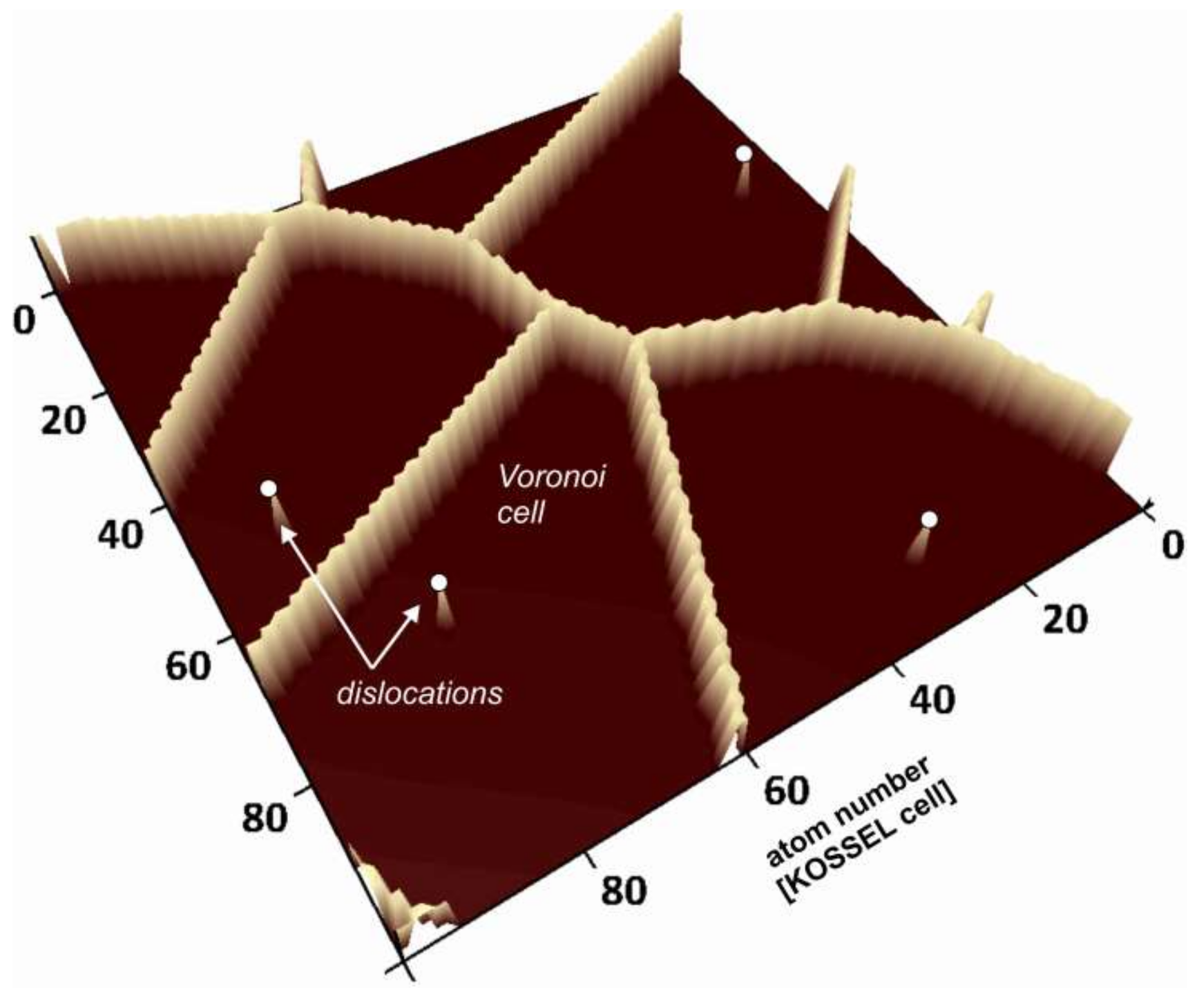
Figure 1 shows an example of a
Voronoi diagram. In an unweighted
Voronoi diagram like this, the
Voronoi cell boundaries are defined as the set of those points having the identical Euclidean distance to more than one generating point. Our kMC calculations employ periodic boundary conditions. Thus, for a quantitative comparison, the
Voronoi cell calculations need to establish periodic boundary conditions as well. This condition was met by providing eight copies of the model grid and arrange it in a matrix that consists of 3 × 3 model grids in simple translation. Calculations of the Euclidean distances thus included all generating points of the surrounding grid copies. In order to analyze the evolution of the crystal surface during dissolution, we calculated 2D distance maps containing information about the distance of each surface point (
x,
y) to the nearest defect outcrop to (
x,
y).
2.4. Weighted Voronoi Diagrams
Isolated etch pits can be treated by using the simple approach of a distance map as explained above. In this case, a simple distance function (metric) containing all the parameters that influence etch pit shape must be obtained. In the more complex case of heterogeneous growth of multiple etch pits, an improved
Voronoi approach is required. This approach must describe the modification of
Voronoi cell shape and size to reflect the heterogeneity in behavior of the growth of etch pits. Thus, the concept of “weighting” is applied. In addition, etch pit coalescence must also be considered. While the opening of pits is tied to defects and hollow core opening [
28], the growth of pits is a stochastic process. kMC simulations reflect this stochastic behavior by the application of random numbers [
10].
Voronoi simulations, however, implement the stochastic parameter by a range of weighting factors (e.g., [
29] and references therein). Usually, etch pits show variable distances of their cores, thus they coalesce having different sizes [
30]. This fact and the resulting variability in kink site density impact the variability of the surface reaction rate, i.e., the variability of the material flux [
31].
Weighting factors reflect this variability in Voronoi maps. Assigning a “weight” to the distance to a certain defect means selectively modifying its distance function after some rule. It can be done additively, multiplicatively, or any combination of both. In this case, acknowledging that it is only the absolute depth—but not the overall shape—that distinguishes a given etch pit from others, an additive weighting that alters only the depth at which the pit is formed is used. Here, an increase in depth and diameter of a pit is represented by a larger weighting factor. The respective defect length is also parameterized in the Voronoi code. In this study, the weighting factors are obtained and calibrated from kMC simulation results. The standard method to provide weighting factors by the kMC code is as follows: (i) calculation of etch pit depths, (ii) calculation of average etch pit depth, (iii) compute the ratio of etch pit depths to that of the average. The result is a set of normalized weighting factors. As a result, the weighted Voronoi diagram is based on both the distance function and the weighting factors, which are independent of each other.
In this study, the bond strength was chosen to be sufficiently large to generate mostly straight steps, resulting in etch pits with essentially a square-shaped outline. To describe this shape properly, the maximum norm was used instead of the Euclidean norm, as the latter would generate circular iso-lines.
2.5. Surface Roughness Parameters Based on kMC vs. Voronoi Results
In this study, we apply standard roughness parameters such as the peak-to-valley depth
Rt, the root mean square roughness
Rq, the interfacial area ratio
F, and the average height
z. For more information about these well-established statistical parameters see [
32]. We calculate these parameters from surface topography data based on both kMC and
Voronoi simulation results. We further compare these results to quantify the differences in the evolution of surface topography using both simulation methods.
The average height
z is defined as:
Rt is defined as the height difference between the highest and the lowest point of the surface:
Rq is defined as the standard deviation, in this case from the mean height
µ of the surface:
F is defined as the ratio of the curved surface area to the flat surface of identical field-of-view:
To determine the curved surface areas of both KMC-generated and Voronoi-generated surfaces, an approximation was made using a triangulation method, summing the triangles spanned by an atom, its right neighbor and its neighbor on the upper right and the triangles spanned by an atom, its upper neighbor and its neighbor on the upper right.
2.6. Theoretical Considerations
To generate the height of a dissolving crystal surface by Voronoi calculations, the height H at a given surface point (x, y) has to be plotted as a function H(r) of the distance r between (x, y) and the nearest defect position (D1, D2). The nearest defect to (x, y) is identified as the one whose Voronoi cell (x, y) belongs to.
Although the exact distance functions are as yet unknown, the relationship between the stepwave velocity and the distance from the hollow core center,
can be computed from the stepwave model [
12]. Here
rcrit is the critical distance at which the hollow core opens, and reflects the material, solution chemistry, saturation state and other environmental parameters. We chose not to use the more accurate but also more complicated formulations for the stepwave velocity also given by Lasaga and Luttge [
15] including ΔG and strain parameters, because the strain influence is largest close to the defects, where the
Voronoi approach does not make any statement anyway. This was deemed appropriate given the trial basis of this
Voronoi model.
The critical question, determining whether it is at all feasible to calculate absolute surface heights at a given time
t using kinetic parameters, is how to compute
H(
r) from
v(
r). To determine the height, it is necessary to know how many atoms have been removed at position (
x,
y) after time
t. Until some critical arrival time
arr(
r), no steps will arrive. The critical time then denotes the initial appearance at position (
x,
y) of a step generated by the defect. To compute the value
arr(
r), we compute the sum of times the step spent traversing infinitesimally small intervals of the total distance traveled. Mathematically, this corresponds to the area below the graph of the inverse values of
v(
r).
As the whole velocity formula is only defined for
r >
rcrit, there is no validity problem and the integral value taken between
r and
rcrit is
with only positive values (
) as arguments to the logarithm. However, this treatment makes no statement as to the behavior at very small distances, lower than
rcrit. This can be deemed acceptable under far-from-equilibrium conditions, as velocities in this region are so fast anyway that the hollow core can be considered as opened almost immediately.
The height at time
t can be calculated directly from the arrival time
arr(
r) as a function of the distance
r to the nearest defect, by
with
H0 being the original height of the cleavage surface, and
v(
rpit) the global retreat rate after the stepwave model [
12], which is defined as the velocity of a single stepwave directly at the critical radius of an etch pit. The stepwave model also assumes this to be the overall rate of step generation and, directly following from this, also the overall velocity of surface retreat. It should be noted that the “measured” global retreat rate in kMC simulations was not constant but showed a huge variance, so for comparison, we fitted it instead on a case-by-case basis by changing the parameter in the
Voronoi software.
The distance
r between a defect (
D1,
D2) and a surface position (
P1,
P2), as mentioned in
Section 2.4, was defined as the maximum norm.
The resulting formula H(r,t) is now the distance function used throughout the Voronoi simulations.
The following parameters from
Table 1 were used for calibration of the distance function and for weighting.
2.7. Weighting of the Voronoi Distance Function
Voronoi distance maps are a mathematical method for the geometrical analysis of data. Using this method for the quantitative analysis of the evolution of reacting crystal surfaces requires the implementation of a kinetic term. Otherwise the Voronoi calculation would provide only a static geometric description of the surface. More specifically, the introduction of the variability in etch pit evolution of crystal surfaces into the Voronoi distance map approach depends on the weighting of the distance map.
Here, we demonstrate different types of weighting and how they can influence a simple Euclidean
Voronoi diagram.
Figure 2 illustrates the impact of weighting factors on the
Voronoi cell shape and size.
As a starting point,
Figure 2A shows an unweighted
Voronoi diagram using Euclidean distance in the plane. The
Voronoi distance map is calculated simply by calculating the distance from each (
x,
y) position in the plane to each defect, and choosing the minimum. The defect in question then defines the
Voronoi cell a point (
x,
y) lies in. The lines of the
Voronoi diagram are theoretically defined as the points having equal distance to at least two defects. In discretized (
x,
y) coordinates, boundary points are defined as points (
x,
y) that possess a minimum of one direct neighbor (upper, lower, left, right) residing in a different cell.
An unweighted Voronoi diagram can be considered as a multiplicatively weighted Voronoi diagram with all weighting factors set to 1, or an additively weighted Voronoi diagram with all weighting factors set to 0.
Figure 2B shows a multiplicatively weighted
Voronoi diagram of the identical crystal surface, however, a weighting factor
w = 1.1 has been assigned to the lower left defect, and
w = 0.9 to the uppermost one. These values were chosen arbitrarily for demonstration purposes. A multiplicative weighting factor operates as a function of distance. More specifically, if a generating point P has a given multiplicative weighting factor
w then all distances to P are divided by
w.
Figure 2C illustrates the additive weighting. If a generating point P has an additive weighting factor of
w in terms of
Voronoi distances, then
w is subtracted from all distances to P. In our example, an additive weighting factor of 5 is assigned to the lower left generating point, resulting in the enlargement of the corresponding cell. With this type of weighting, the variability in cell size reflects the stochastic behavior of surface reactivity close to a defect. A small cell, generated with a low weighting factor, reflects a defect with a small region of influence with respect to the material flux during dissolution, and vice versa. As a consequence, the cell surrounding a defect with a larger weighting factor represents faster (lateral and vertical) pit growth. This relationship illustrates how weighting factors encode the variability observed in experimental and kMC studies.
Finally,
Figure 2D shows results calculated using a combination of additive and multiplicative weighting factors having a larger range compared to
Figure 2B,C. This image illustrates the variation in functions used for different types of weighting. Note that the lower left generating point in
Figure 2D has so much weight that the corresponding cell ranges across the entire system size.
In this study, we use the maximum norm as distance. This means the distance between a point (x, y) and a defect at position (d1, d2) is defined as max(|x − d1|, |y − d2|).
The weighting is then based on kMC results about crystal surface evolution and provides the critical constraints to the kinetic significance of the Voronoi calculation results. We only use additive weighting, reasoning that when etch pits evolve, only their depth changes, but not their overall shape (which would be sensitive to multiplicative weighting). Thus, the weighting encodes the specific reaction kinetics of the system, representing the variance in growth speed of particular etch pits. In this study, to gain a comparable dataset, weighting factors for the Voronoi calculations were gained from kMC by setting the absolute depth of single etch pits relative to that of the average etch pit depth.
3. Results
To summarize the details of our approach, we analyze the capabilities of Voronoi diagrams in terms of the quantitative analysis of crystal dissolution reactions. We utilize kinetic Monte Carlo (kMC) simulation results for the kinetic parameterization of Voronoi diagrams. We apply kMC data of etch pit depths after given reaction periods for the calibration of weighting factors of the Voronoi diagram, generated from the Voronoi distance function. In so doing, we demonstrate that the prediction of the inherently complex kinetics of surface reactions can be reduced to the problem of determining these weighting factors. As a step forward, we show that the variability of etch pit growth and coalescence can indeed be described by the weighting factors of Voronoi diagrams using a specific distance function. This distance function thus encodes physicochemical and material properties of the crystal lattice and its reacting fluid.
3.1. Comparison of Surface Topographies Simulated by kMC vs. Voronoi Techniques
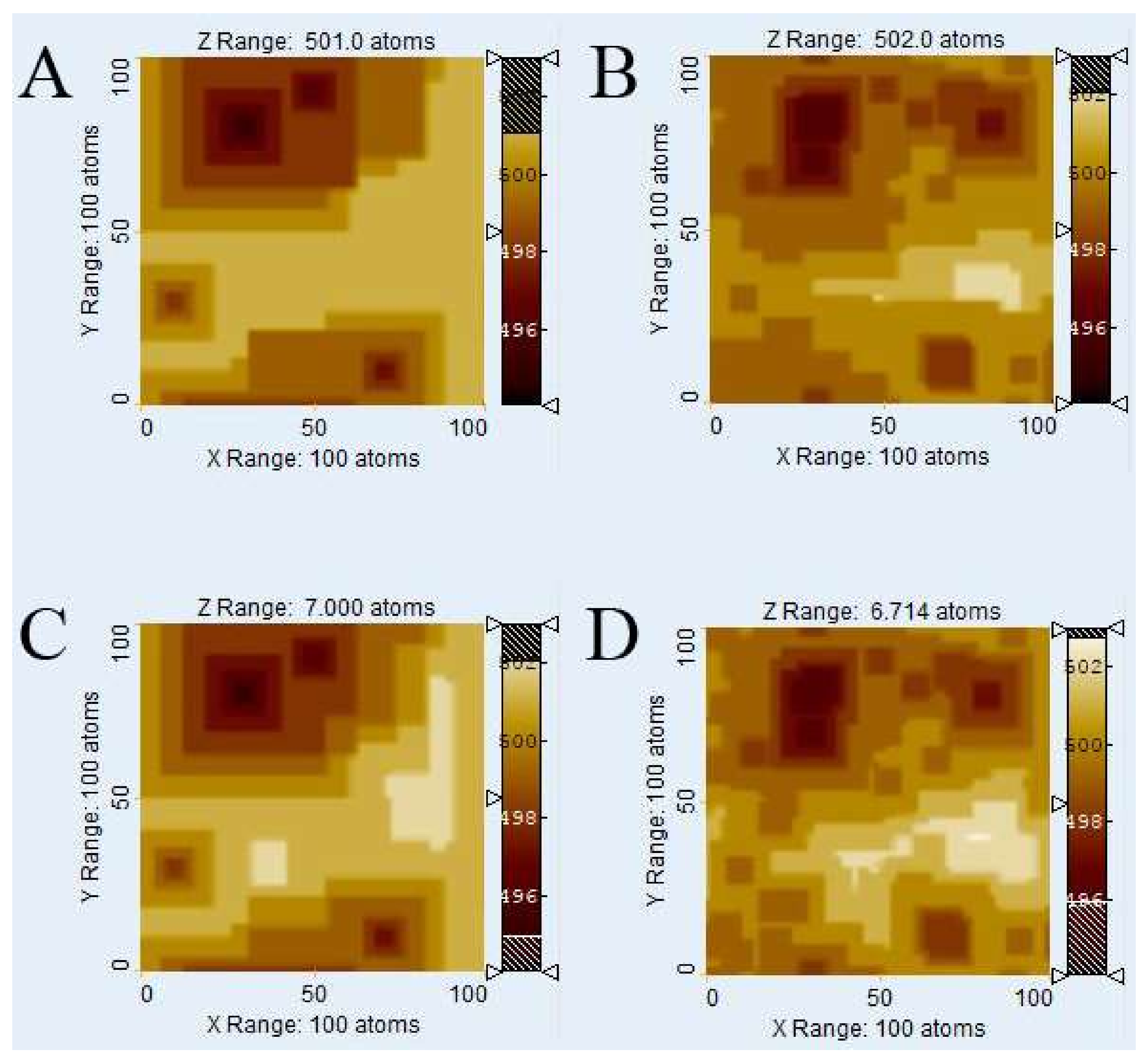
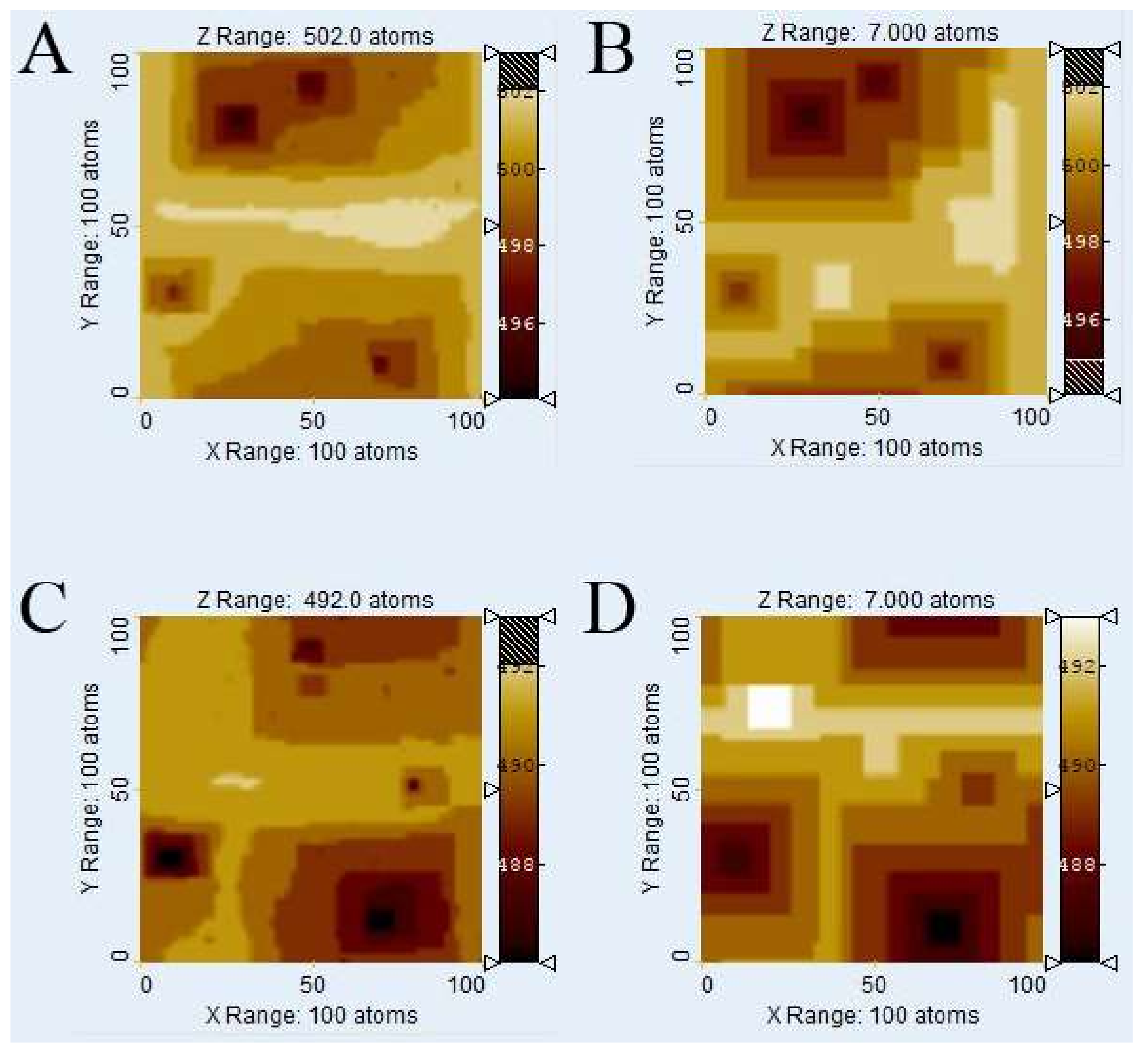
Figure 3 illustrates the evolution of
Kossel crystal surface topographies using kMC and
Voronoi techniques after dissolution of 1 × 10
6 atoms. The kMC simulation results (
Figure 3A,C) were used to calculate weighting factors for the
Voronoi distance function from the depth of etch pits. Also, the parameters of the distance function were fitted by comparison with kMC surface morphologies, first roughly by visual comparison and then fine-tuned by comparing histograms.
Figure 3B,D show the corresponding surfaces generated by the
Voronoi calculation using the weighting factors from the kMC runs in
Figure 3A,C, for relevant calibration parameters see
Table 1.
Figure 3E,F show the cell boundaries of the corresponding
Voronoi diagrams.
Visual comparison of kMC and
Voronoi generated surfaces shows already that this parameter fit of the distance function is able to correctly reconstruct the depth and width of etch pits, both in the case of low versus high defect density (
ndefect = 4;
Figure 3A,B vs.
ndefect = 40;
Figure 3C,D). In the case of high defect density, the kMC results indicate that not all defects produce etch pits. This has been observed previously, and reflects the nature of kink site distribution. At a pit wall with high defect density, the step velocity is comparably high, thus hindering the growth of new pits. This is illustrated in
Figure 3C where several defect outcrops without any significant pits are visible. The
Voronoi model deals with this phenomenon by assigning small weighting factors to those defects. The corresponding
Voronoi cells do not disappear but are relatively small. However, a defect may become “reactivated” later, provided it is sufficiently long, and that growth of the corresponding pit (and
Voronoi cell) are kinetically feasible. A significant visual difference between kMC and
Voronoi surface morphologies is the smoothness of steps in the
Voronoi results, reflecting the lack of stochastic events on the surface.
Due to the statistical nature of kMC simulations, no valid absolute correlation coefficients between kMC and Voronoi calculation results can be calculated, as they would differ with each kMC run. However, a slight tendency towards a dissimilarity in areas outside the immediate vicinity of an etch pit at higher defect densities has been observed. Potential explanations include either an inaccuracy in the chosen distance function or the dominance or stability of local surface plateaus related to step bunching, complex interactions that are not yet explicitly implemented in our current Voronoi model.
3.2. Defect Density, Etch Pit Coalescence and the Influence of Simulation Time
Figure 3A–D shows that the morphological similarity between kMC and
Voronoi-based surfaces decreases with higher defect densities, i.e., for more complex surfaces incorporating a higher number of
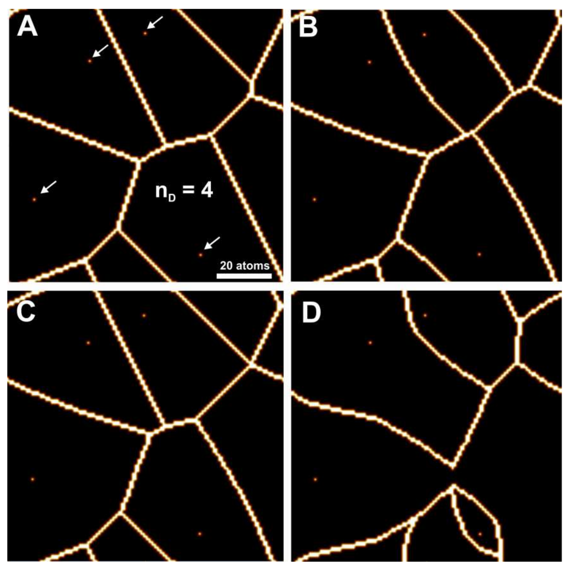
Voronoi cells and more influenced by the coalescence of etch pits. Because of this, etch pit coalescence was treated separately, using a high bond strength to generate purely square etch pits.
Figure 4 shows coalescing square etch pits,
Figure 4A for 4 defects and
Figure 4B for 40 defects, having otherwise the same parameterization as in
Figure 3B,D. As there is no theoretical description of the velocity of fast steps, in this case their velocity was assumed to be infinite (i.e., the time required for their surface transit is zero). The actual surface will be somewhere between these and
Figure 3B,D respectively. For illustrative and statistical purposes,
Figure 4C,D show the average values of the coalesced and un-coalesced
Voronoi surfaces. These images are imperfect in their representation of step morphologies, but do define areas of etch pit coalescence observed in the kMC simulations. It should be noted that the actual kMC results can vary significantly, so this approximation was considered acceptable.
Figure 5 shows an analysis of the
Voronoi method’s applicability at different extents of reaction, here represented by different numbers of removed atoms. We tested, for the system with 4 defects, the timeframes of 10
5 removed atoms (
Figure 5A,B) and 2 × 10
6 (
Figure 5C,D) removed atoms, the latter being identified as the largest possible value at which the kMC method still generally yielded plausible results at the chosen system size and conditions. (Letting the simulation run longer sometimes generated a feedback loop that caused artifacts. We thus avoided longer runtimes because we could not guarantee the validity of the results).
Clearly, the visual similarity of kMC (
Figure 5A,C) and
Voronoi (
Figure 5B,D) results is neither better nor worse than the comparison for 10
6 removed atoms (
Figure 3 and
Figure 4). This means the
Voronoi method is generally suitable at the very least for the range at which the kMC method at this system size is valid.
All but one of the distance function parameters (disregarding the completely unrelated weighting factors) were unchanged– except the very critical
v(
rpit), which seems to diverge, as seen in
Table 2. The other fitting parameters (
rcrit and
vstep) stayed the same, independently of simulation time. The parameter
v(
rpit) is slightly different for each run (neglecting a complete variance analysis), and becomes higher at longer simulation times. This result may indicate a change in surface reactivity with surface roughness and kink site density. Although it is hardly surprising that reactivity, site distribution, and topography change in lockstep with one another, the identification of a single model parameter, whose variation can produce the spectrum of observed results while other parameters remain fixed, is itself an interesting result warranting further examination.
No other irregularities or diverging parameters were observed, which means v(rpit), was the only distance function parameter that must be re-fitted for each kMC run, which indicates a potential role of v(rpit) as a potential “culprit” bearing responsibility for the large variation observed in simulated and experimentally observed rates. Unfortunately, no way exists so far to predict this parameter and its complex behavior. More work on this topic, including the generation of larger amounts of data and variance analysis, is clearly needed for future work. The irregular behavior of the parameter itself, however, is not intrinsic to the Voronoi method—the data here comes from kMC simulations.
Figure 6A shows the probability of a kink site being present at a certain location, expressed as the distance to the nearest defect. Data were taken from the kMC simulation with 4 defects and 10
6 removed atoms.
Figure 6B shows the probability of a ledge site being present at a certain location, plotted against the distance to the nearest defect. The diagrams show a clear tendency for the occurrence of ledge sites: it is more likely for a ledge site to occur in close vicinity of a defect versus some distance away. This result reflects the spatial heterogeneity of reaction rates. The kink site statistics do not show this kind of trend when considering a pre-reacted surface. As dissolution begins, kink sites occur more frequently near a screw dislocation. With continued reaction progress, this trend disappears. Rate is not independent of kink site density; instead, local rate differences as a function of distance to defect centers are small compared to overall retreat and variations in surface normal retreat linked to the appearance and disappearance of etch pits.
Both kink and ledge site distributions determine how fast a material dissolves. A correlation between the kink and ledge site probabilities, together with their corresponding local reaction rates, as a function of defect proximity offers insight into the relationship between reaction rate and defect distribution. The difference in ledge site probabilities shows that etch pit shape is sensitive to surface retreat.
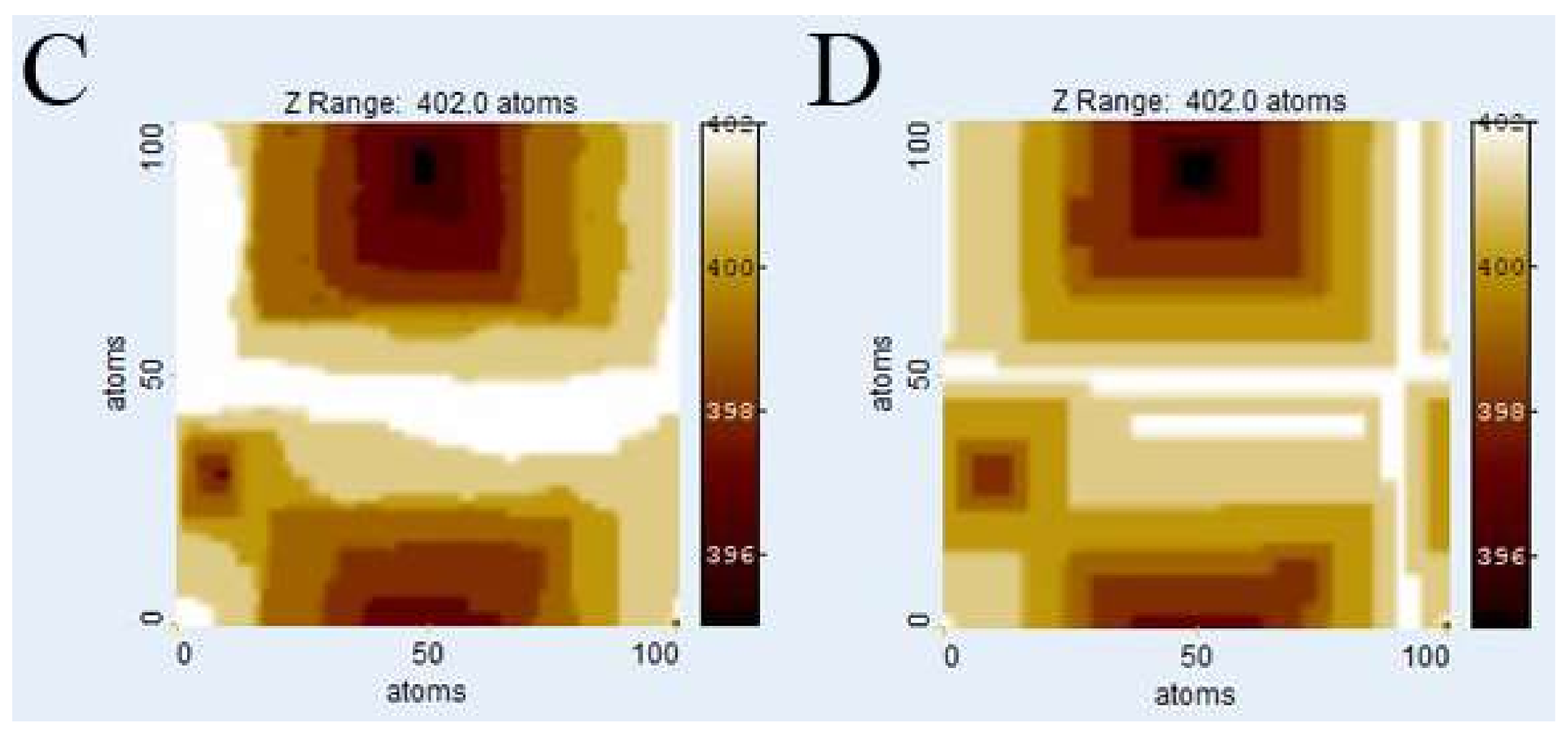
3.3. Evolution of Etch Pits at Defects with Well-Defined Lengths
We now analyze systems having defects with varying length. Here, the results from the kMC run from
Figure 3A were taken (4 defects, topography after dissolution of 10
6 atoms). One of the defects in the upper left has run out, thus is no longer source of step waves. After a new hollow core opened in the middle of the right side, the simulation was continued for a period of dissolution that includes removal of additional 10
5 atoms. To produce the corresponding
Voronoi diagram, new weighting factors were applied, using calculations previously described in
Section 2.4.
Figure 7 shows kMC and
Voronoi simulation results after removal of 10
5 atoms, as in
Figure 6. The etch pit in the upper left section has flattened, because the defect does not persist with depth (
Figure 7C,D). The pit grows laterally but no new step waves are generated, so during dissolution, the pit does not grow into depth anymore and the morphological impact of the pit will disappear as soon as the higher parts of the crystal topography get dissolved.
Another situation is the formation of new etch pits when a new defect outcrop becomes accessible to surface dissolution. For example, in
Figure 7D (middle right of the image), a new etch pit appearing at the newly exposed screw dislocation defect is still smaller compared to the surrounding older etch pits. Both simulation techniques illustrate the formation and evolution of new step waves emanating from this defect. The new step waves are still small compared to those from the existing pits but will travel over the surface and their interaction with other step waves will result in the evolution of a rather complex topography at this surface section. Our point here is that the current
Voronoi calculation is capable of representing the complex interaction of multiple defect structures of variable finite length, a basic requirement for the calculation of flux, rate maps, and rate spectra.
3.4. Comparison of Material Flux and Rate Maps
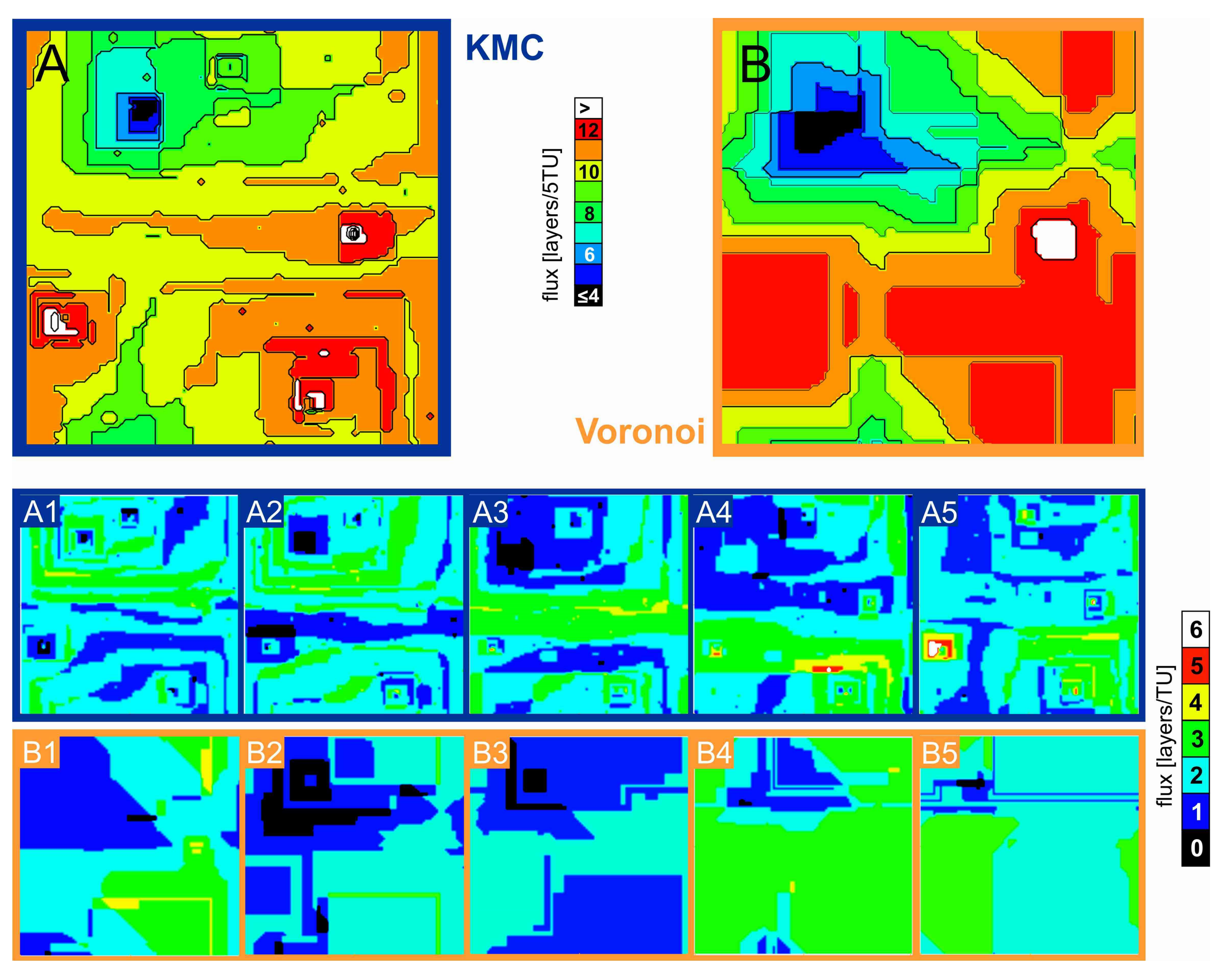
Figure 8 shows a comparison of material flux maps of the reaction period equivalent to the removal of 100,000 atoms, starting from the surface situation of
Figure 3A,B, in 5 steps that log the removal of 20,000 atoms each.
Figure 8A (A1–A5) shows the material flux map of the kMC simulations and
Figure 8B (B1–B5) shows the corresponding
Voronoi simulations, using
v(
rpit) data obtained from the kMC results. The newly opening etch pit is also observed in both kMC and
Voronoi calculations.
The resulting overall rate maps (
Figure 8A,B) have in common that they identically identify the identical areas of high or low material flux, respectively. They both identify the lowest material flux in the upper left, which is the position of the closing pit. They also both see the highest material flux in the vicinity of the lower two still active etch pits and the newly-opened hollow core and associated etch pit (see
Figure 7 for comparison). Interestingly the shorter-time kMC simulation sequences (A1–A5) do not look all too similar to their
Voronoi counterparts (B1–B5)—A1 looks nothing like B1, and A4 looks nothing like B4—however, the overall flux “averages out” so the resulting images (
Figure 8A,B) look very similar again.
Due to the distance function used (the maximum norm), the Voronoi rate map shows mostly straight lines separating areas of different material flux. These boundaries are rougher in the kMC flux map due to the statistical nature of that method.
Any edges in the Voronoi flux map that are not completely straight are a result of averaging the simulation results with and without incorporating etch pit coalescence. Interestingly, this simple method is already able to reproduce the position, and at least roughly the shape, of irregularly shaped surface features like e.g., the green “wedge” in the lower left.
The main statistical difference between the different types of simulation is that the
Voronoi approach appears to systematically overestimate the spatial extension of extremes (areas of particularly high or low flux) and underestimate the extension of plateau areas (yellow areas in
Figure 8A) that are not close enough to a defect position to be considered as lying inside an etch pit. This might be partially due to a misfit of the distance function used; however, more likely it is a result of using a simplistic kMC model that only considers first neighbors.
Also, when looking at shorter reaction periods (
Figure 8A,B (A1–A5 and B1–B5)) the differences between the flux maps of kMC and
Voronoi simulations become more pronounced. This is mainly because the
Voronoi calculations only allow for the simulation of the retreat of etch pits of constant shape. The kMC simulation, however, produces fluctuations in etch pit shape, as well as the development of step roughness, heterogeneously distributed over the surface. Over a shorter time span, the statistical influence of those fluctuations obviously must be more pronounced. Also, there are sometimes differences in the total surface retreat (esp. comparing
Figure 8 A4 and B4) that depict a fluctuation in overall surface retreat. This rate variance cannot be reproduced in detail by
Voronoi calculations. We thus conclude that the larger the time interval is chosen, the higher will be the similatity of kMC and
Voronoi flux map.
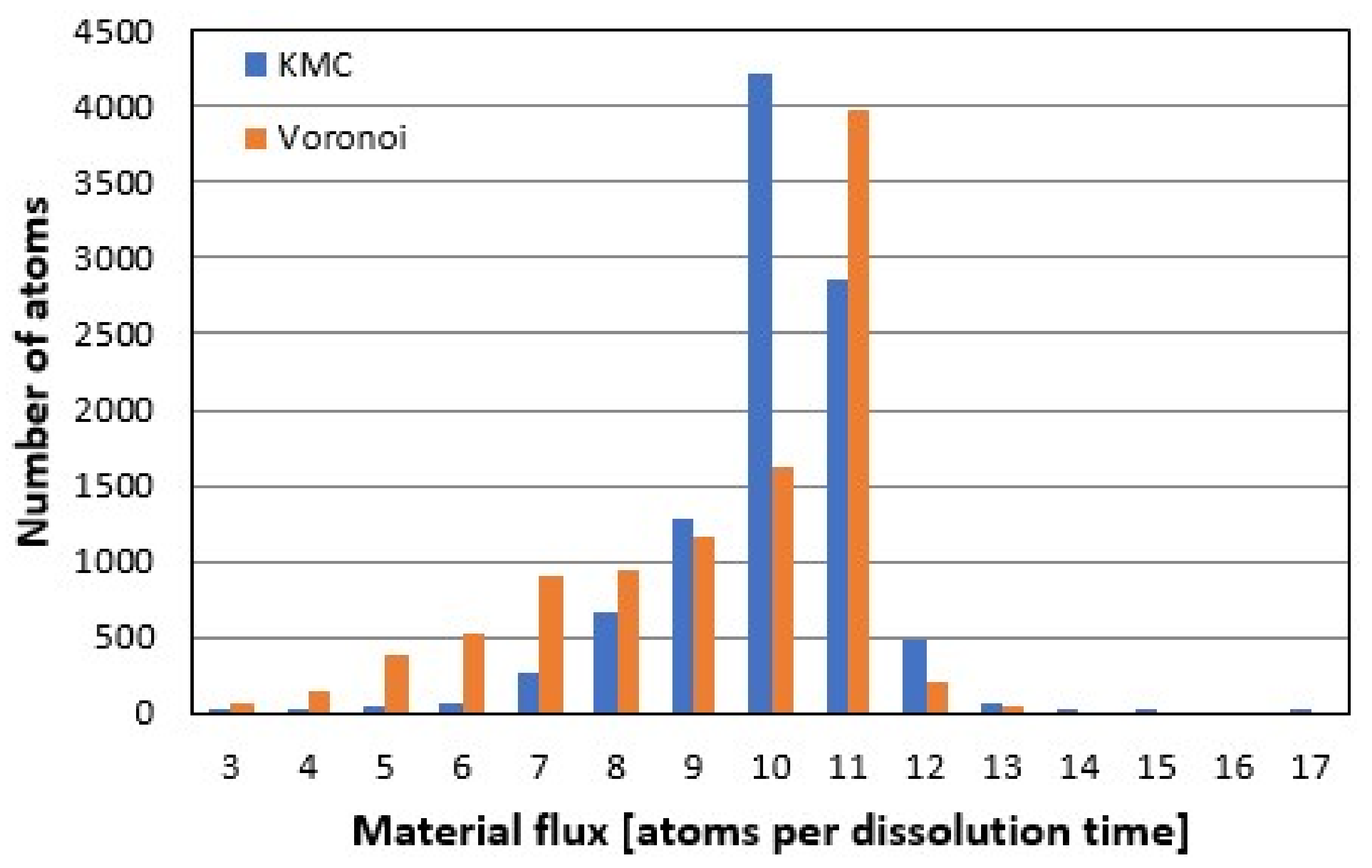
3.5. Comparison of Rate Spectra Results
Analyzing the material flux or reaction rate maps (
Figure 8) in the frequency domain leads to the histogram of rate contributors, i.e., the rate spectrum.
Figure 9 shows a comparison of the kMC- vs.
Voronoi-based rate spectra after removal of 10
5 atoms, starting from the pre-reacted surface in
Figure 3A. The crystal structure includes four screw dislocation defects, as shown in
Figure 7C,D. The
Voronoi peak is sharper due to the lack of randomness inherent to stochastic methods like kMC—so although the exact surface heights are not exactly reproduced in their inherent randomness, rate contributors are correctly identified. The slight difference in peak position of one atomic layer might be due to the still rather rough treatment of etch pit coalescence and the as yet inaccurate reconstruction of the material flux on plateaus, as seen in
Figure 8A,B, or due to different modes.
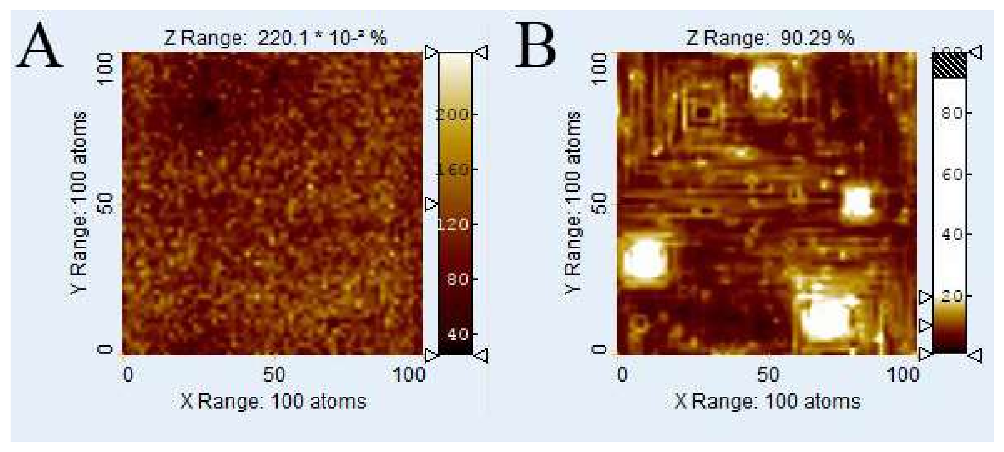
3.6. Kink Site Density
Figure 10 shows the kink site density (
Figure 10A) and ledge site density (
Figure 10B) during the run of a kMC simulation, from the same dataset as
Figure 6 and
Figure 7, plotted against the distance to the nearest defect.
Figure 10B shows it is far more likely for a ledge site to occur near a defect than far away from it.
The kink site density does not show such a clear pattern—the only visible feature in
Figure 10A is a patch of apparently lower than usual kink site densities in the upper left, which is the area where an etch pit disappeared. The pit that was widening but not deepening any more shows far lower kink site density than the dissolving plateaus. Otherwise, the positions of defects are not clearly discernible from simple inspection of kink site density.
3.7. Parameter Variation and Sensitivity Test of the Fitting Function
We analyze how the distance function impacts the calculation of the rate range of the
Voronoi-based rate spectra. In general, the fitting function describing the general shape of etch pits in the examined example system depends primarily on the parameters described in
Table 1, using the distance function in Equation (8) with
H0 set to 600 as an input parameter, and
t taken from the kMC simulation result.
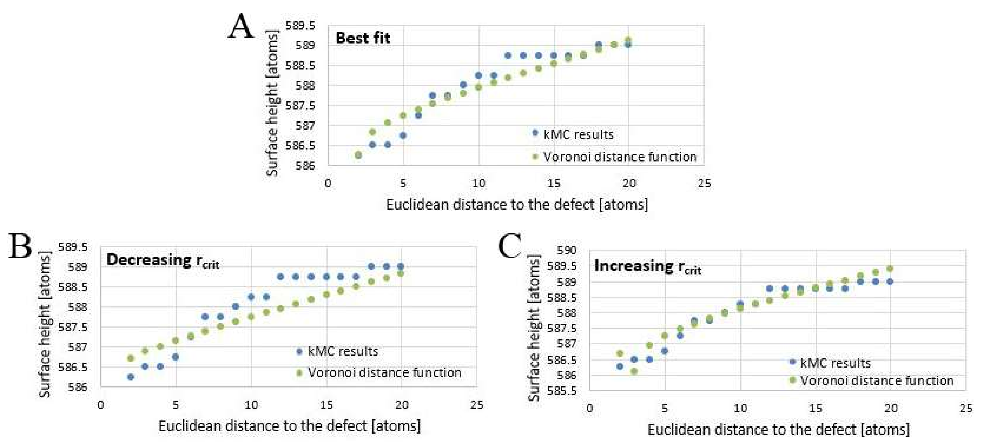
In this case, we consider the example of one single etch pit in the middle of a 101 × 101 Kossel surface with periodic boundary conditions, after a dissolution of 105 atoms. This fairly short period was chosen to prevent step bunching phenomena. The kMC heights at a certain distance r to the defect (51, 51) were calculated by using the mean value of the heights at the positions (51 + r, 51), (51 − r, 51), (51, 51 + r) and (51, 51 − r). These values were then used to fit the distance function. Three parameters were manually varied for the fit are: the rate of generation of new stepwaves v(rpit), the straight step velocity vstep, and the critical radius rcrit.
The “optimized” parameters were gained by manual testing of the changes occurring when iteratively changing parameters. This could be done directly in Excel by varying the function input—the three varied parameters could in this case be treated independently of each other because their effect on the overall function differed not only quantitatively but also qualitatively. It was thus possible to incrementally change parameters and record results. The fit was considered “best fit”, when small changes in one of the three fit parameters caused visible deviations of the fit function values from the kMC results.
The best fit (
Figure 11A) for this particular kMC run was obtained with
rcrit = 1.9
Kossel units,
vstep = 2.9 × 10
−8 Kossel units per second, and
v(
rpit) = 2.98 × 10
−9 Kossel units per second, although it should be noted that the stepwave generation velocity
v(
rpit) not only showed a high variance when repeating the kMC simulation with identical starting surface, but also appeared to depend in some yet unknown way on defect density. A tendency towards higher
v(
rpit) at higher defect densities (with
rcrit and
vstep staying the same) was observed.
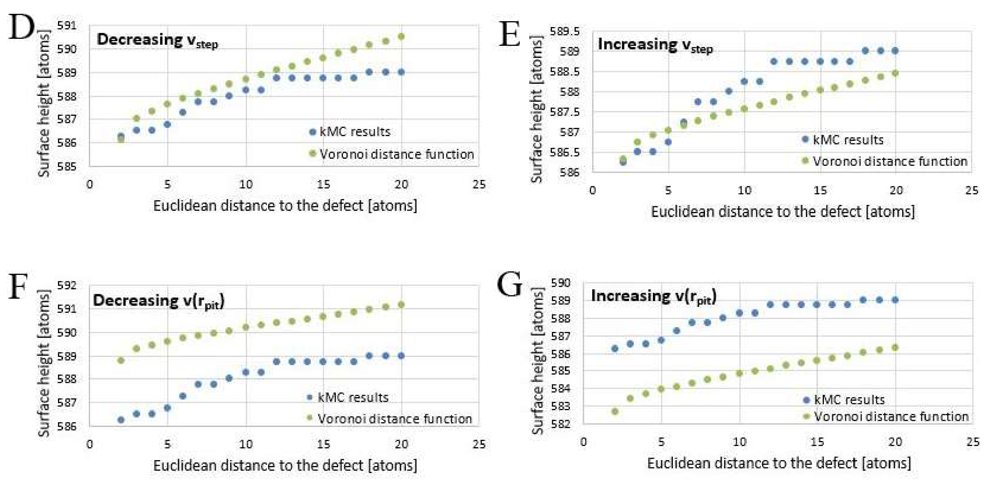
Varying the fitting parameters yields different results. To illustrate this, starting from the best fit, the following
Figure 11B−G demonstrate the outcome of arbitrary changes in fit parameters from their optimal “best fit” value.
Decreasing
rcrit to 0.9 (
Figure 11B) flattens the graph of the distance function; increasing it to 2.9 (
Figure 11C) yields a misfit close to the core and makes the graph appear steeper. Decreasing
vstep to 1.9 × 10
−8 Kossel units per second (
Figure 11D) steepens the pit walls, increasing
vstep to 3.9 × 10
−8 Kossel units per second (
Figure 11E) flattens them. Decreasing
v(
rpit) to 2.43 × 10
−9 Kossel units per second (
Figure 11F) raises as well as flattens the fit function, increasing
v(
rpit) to 3.75 × 10
−9 Kossel units per second (
Figure 11G) lowers it.
3.8. Comparison of Surface Roughness Parameter Results
We compare
Voronoi and kMC based roughness parameter results as a measure of similarity versus dissimilarity between surfaces generated by kMC and
Voronoi methods, see
Table 3. The data are taken from removal of 10
6 atoms from a 100 × 100 surface.
Voronoi calculations are again the resulting surface of the average of coalesced and un-coalesced surface as described in
Section 3.2.
The average surface height
z is in both cases almost identical for
Voronoi and kMC calculations. The
z value must be close to 500, because starting height was 600 and 1 million atoms were removed over a 100 × 100 surface. (It is not exactly 500 due to the presence of hollow cores (kMC), and in the
Voronoi case, a slightly different rate spectrum.) The reacted surfaces have roughly the same height, meaning a very similar amount of total removed atoms. This is not surprising, considering the
v(
rpit) values, which determine the overall surface retreat, were taken from kMC for the
Voronoi calculations. The roughness parameter
z is reproduced best. The small difference is most likely due to inexact identification of plateaus, as also observed in
Figure 9. The parameter
z affords no control over the spatial distribution of material flux.
The roughness depth Rt data (Equation (2), Methods chapter) show a clear tendency towards lower values in the Voronoi simulation. This is because the Rt value, the difference between the highest and the lowest points on a surface, is very sensitive to minima and maxima. Voronoi simulations can reconstruct the general topography of a surface. However, misfit of the lowest valleys inside the pits, which affected very few atomic positions, was found. Single (x, y) point surface peaks are difficult to reconstruct by the current Voronoi simulations, as shown by the Rt deviations. An improvement of the fitting function, maybe also using more parameters, might be able to correct such deviations, although the algorithm will never be able to calculate the lowest values inside the critical radius of etch pits.
Systematically different results were found for the
Rq parameter data (see Equation (3)), which means that although the general topography in terms of “hills and valleys” is constructed correctly, the distance function still shows some inaccuracy in describing the general pit wall shape. Because of the square term in Equation (3) the
Rq value would be very sensitive to maladjustments of the distance function. Also, as observed in
Figure 8, the tendency of the
Voronoi calculations to underestimate the spatial distribution of plateaus and overestimate the size of areas with especially high or low material flux will systematically support too high
Rq values.
The comparison of surface factors
F yields a critical property of the
Voronoi approach. Results of
F based on
Voronoi surface data without coalescence are always smaller compared to KMC results (see
Figure 3A,B as an example).
Voronoi simulations do not consider step roughness, thus smoothing the topography of pit walls. The values are similar when comparing the averaged
Voronoi surface (see
Section 3.2) to the kMC-generated
F value; however, this is most likely due to artifacts. It is not possible to draw any conclusions about similarities from a similar
F value. Small-scale roughness is not part of the calculation that focuses on the height values as a function of the distance to a defect.
Overall, the comparison of these surface roughness parameters as a plausibility check shows a good correlation. The areas of higher or lower reactivity are correctly identified, so are the overall surface structures. However, the
Voronoi approach does not consider the smallest-scale phenomena, such as kink sites or single steps moving over the surface—phenomena like step roughness cannot be described with this method, which becomes obvious especially when looking at the material flux sequences of
Figure 8.
4. Discussion
4.1. Comparison of the Run Time of the Voronoi and kMC Methods
The main advantage of Voronoi calculations is their efficiency and simplicity. For our examples, when measuring simulation times of 1 million removed atoms, the ratio of simulation time of Voronoi and kMC methods is about 1/180, i.e., the Voronoi method calculation requires about 0.5% of the computational power used for the kMC calculations. Voronoi simulation will always be faster because it only needs to calculate the surface morphology at the final stage of dissolution that needs to be observed, without having to simulate all the steps in between. The speed of Voronoi algorithms can be attributed mainly to two factors:
(i) Calculations do not require additional calculation time for removing more atoms, i.e., simulation longer periods of reactions. For the kMC method, it is necessary to make lists of all possible events that can happen at every step of dissolution (every removal of one atom), as well as their rates and the total rate sum (see e.g., [
33]). This is a time-consuming process that grows linearly with longer dissolution time. The
Voronoi algorithm only considers geometrical defect positions, but not lists of events and rates. It is thus completely independent of temporal scale.
(ii) KMC calculations become significantly slower if one considers more parameters, e.g., the solution chemistry, because this requires more possible types of events to be considered in the simulation. A key decision for kMC simulations of large, complex systems is the choice of which types of events to include (see [
14]). In an ideal case, the potential energy surface (PES) after any possible transition would be known [
33]—however, practically, that is not feasible. In
Voronoi calculations, however, any such parameters are considered within the distance function, even though the parameters for this function must come from KMC calculations. The required computational power is little impacted by the complexity of the distance function—in any case, only the distance map pertaining to one single etch pit will have to be calculated once, and then stored and re-used.
The size of systems that can be observed via kMC simulations is rather limited due to the necessity of treating a large number of possible events in the system and storing information specific to each lattice site. Although kMC programs can be sped up and the system size can be increased, for example by parallelizing the code, the parallel algorithms have a number of efficiency and scalability drawbacks [
34], as well as theoretical issues, such as obeying detailed balance principle [
35].
Kossel-type kMC models in the literature have typically sizes up to 4000 × 4000 atoms [
15]. State of the art kMC simulations (usually using a cluster or computation center) of real minerals typically have the size of a few hundred units in each direction. As an example, Kurganskaya and Luttge [
36] recently used a model having 600 × 600 × 300 CaCO
3 units for the simulation of calcite dissolution. However, these simulations already require large-capacity computers or compute clusters.
Initially, kMC calculations are required to calibrate the distance function of the Voronoi software. However, this calibration can be performed using a relatively small system size. A challenging problem, however, is the accommodation of interaction between the pits, requiring appropriate adjustments of the time-dependent weighting parameters. This problem requires further methodological and algorithmic development.
In the Voronoi calculations, the practical limiting factor on an ordinary laptop computer proved to also be system size, namely, the size and number of Fortran arrays that could be stored in the computer’s RAM. In this study, the simulated systems were chosen small on purpose: the aim was to create a simulation method that does not depend on access to specialized hardware like a cluster or a computation center. At this point, no detailed analysis of computational requirements has been done, although clearly a larger system needs more resources, and as the number of defects increases, the number of distances requiring calculation also grows. The Voronoi code could be made more efficient by optimizing the Voronoi segmentation algorithm. Lastly, code parallelization could be considered in the simulation of larger systems.
4.2. Advantages and Disadvantages of the Voronoi Approach
The main disadvantage of Voronoi calculations is their inability to account for smallest-scale phenomena. The Voronoi model only yields straight steps, so clearly some information is lost. If information about step roughness is needed, a kMC simulation must be run, and the Voronoi model does not offer an alternative in this case. Also, the Voronoi model makes absolutely no statement about the reactivity of a certain site at a particular time. Any information pertaining to kink site and ledge site distributions is lost. Surface reactivity in the Voronoi model is treated only as height retreat. The single mechanisms leading to the removal of atoms during dissolution are not examined. Any smallest-scale phenomena, as well as roughness parameters pertaining to smallest-scale structures, must be simulated with kMC.
The main advantage of
Voronoi simulations compared to kMC simulations is speed. In fact,
Voronoi calculations will always be faster than kMC due to the elimination of the memory and expensive bookkeeping required for each site configuration, as well as reactivity and recalculation of event probabilities at each simulation step as discussed in
Section 4.1.
Another obvious advantage of the
Voronoi approach is the possibility of having a way to determine the regions of initial influence single defects (as generating points, see e.g., [
29]) can exert over a surface. Although kMC cannot directly do this as no partitioning of the surface is done, the partitioning comes out naturally as a simulation outcome. Over time etch pits compete for the space, coalesce and annihilate each other. This process is captured by the KMC method and observed in microscopic experiments. Since the partition technique offered by the
Voronoi approach is static, the temporal changes of the etch pit dominance fields and etch pit interaction should be taken into account from the relevant KMC studies and experimental observations.
The full potential of this new possibility has not been realized yet, however, there are future possibilities to predict major trends in surface-controlled larger-scale reactivity behavior solely from analyzing the defect distribution of the crystal.
4.3. Plausibility of Voronoi Data
Experimental observations on crystal dissolution far from equilibrium identified two types of etch pits: short-lived ones attributed to nucleation at point defect clusters or impurities, and longer-lived ones attributed to screw dislocations [
37]. The current
Voronoi approach completely ignores the first, but calculates the latter.
As seen above, the gained morphology data, gained simply by calculating an overall shape of etch pits and then superimposing several etch pits over each other as described in the methods section, correlate well with kMC models and can thus be considered plausible on larger scale. Comparison of surface roughness parameters (see
Section 3.8) also demonstrates the correct identification of larger surface features, although smallest-scale features like single steps are lost.
When comparing material flux sequences, it should be noted that while all other parameters stayed identical,
v(
rpit) varied even in this relatively short timespan of 0.27 × 10
10 s, from 3.83 × 10
−9 atoms/s to 3.77 × 10
−9 atoms/s. Repeating the simulation several times also yielded completely different results again. This points into the direction that the huge rate variance of crystal dissolution measured experimentally in many minerals, e.g., calcite [
4] is not only due to extrinsic factors, but a property of the dissolution process itself. No deterministic process of predicting this is known—see
Table 2 for the interesting behavior of
v(
rpit).
When it comes to material flux and histograms, however, the Voronoi data can be considered reliable. Material flux maps are obtained by subtracting two surface morphologies from each other. In that process, smallest-scale structures like single steps will disappear anyway. This means that if you don’t need the smallest-scale information, the method is valid.
4.4. Potential Future Applications of Kinetic Voronoi Calculations
Voronoi calculations, in combination with analytical and experimental techniques, have the potential of offering new predictive properties. The two most important main goals in the future are the application of the new Voronoi method to real-world systems with existing minerals, and the development of an upscaling strategy that allows to link pore scale and continuum scale for the purpose of Lattice Boltzmann and reactive transport modeling.
Simulation of real minerals clearly must be done not only in combination with kMC, but also with laboratory techniques like atomic force microscopy (AFM) or vertical scanning interferometry (VSI). These methods can provide essential data about defect densities and defect distributions as well as reaction kinetics under a certain set of conditions.
When upscaling, Voronoi methods could then be used to connect the different scales at which dissolution is examined. The overall aim must be a coupled model of mineral-water interaction including surface evolution as well as fluid dynamics at a surface that is not flat and changes its morphology during the course of the simulation. The analysis of the velocity field at the mineral surface provides meaningful boundary conditions to solve the hydrodynamics part. This, however, requires a fast way to generate a surface, run a fluid dynamics simulation, and re-generate a slightly different surface that implements changes in reaction rates stemming from changes in flow, which change material transport and influence dissolution rates that way. Simple averaging of surface reactivity and reaction rates may lead to results that do not provide sufficient predictive power. The versatile system sizes of Voronoi approaches, however, provide the opportunity to connect simulation concepts focusing on either crystal surface and pore scale and the continuum scale. First, the kMC-based parameterization of Voronoi simulations facilitates the meaningful information about surface reactivity based on mechanistic constraints, i.e., no simple averaging of surface reactivity. Second, the quantitative analysis of Voronoi-based rate spectra results provides input data for the continuum scale. A critical point in such strategies is the statistical analysis of histogram modes of the material flux maps that are controlling the evolution of the reactivity model at the continuum scale.
Both Lattice Boltzmann (LB) and reactive transport solvers give solutions for concentrations of an element at a space-time point (
x,
y,
z,
t), taking into account dissolution-precipitation processes. LB solvers have explicit grain boundaries and can take into account porosity and space geometry changes, while reactive transport solvers rely on pure differential equations with boundary and initial conditions. Both methods need a space-time resolved information about mass fluxes that are typically derived from an analytical kinetic equation linking environmental parameters, e.g., saturation state or pH, to the dissolution and precipitation rate:
where
n is a “rate order” parameter,
S is saturation state, k is the “rate constant”. Attempts to measure rate constant at the laboratory settings keeping all the environmental parameters controlled, lead to the well-recognized intrinsic rate variance problem [
6]. A thorough quantitative investigation of that problem on carbonate minerals [
10] showed that the variance indeed is related to the intrinsic variance of crystal defect distributions, grain sizes and crystal faces exposed.
The direct implementation of the rate variance concept into the reactive transport and LB solvers is a challenging problem due to several reasons:
- (1)
the ranges of variance at given environmental conditions (e.g., saturation state) are a-priori unknown;
- (2)
there is no available methodological tool allowing us to predict and incorporate rate variance ranges into the solvers;
- (3)
even when such a tool becomes available, the issue of calculation speed and spatio-temporal resolution of that tool becomes a critical and limiting issue.
The KMC method showed its efficiency in explaining and predicting surface topography and reactivity, and, given the molecular reaction rates correctly, kinematics of reactive features, such as steps and etch pits [
15] and material flux rates [
36,
38]. Running a KMC solver, however, at any required (
x,
y,
z,
t) point can be very time consuming and overall challenging and impractical.
On contrast, parameterized Voronoi solver shows a great promise of solving this problem in a fast and efficient way, since it is capable to build surface topography and material flux maps from a simple analytical equation. This tool might be used as a new promising link between the microscopic models of surface reaction processes and pore scale models of material transport.
Key question in that scenario is the so far unsolved question of generating a set of completely synthetic, but plausible, weighting factors for the Voronoi diagram. So far, the rules governing weighting factor distributions are largely unknown. A dynamic approach simulating the distribution by adding a stochastic element to the weighting factor set seems feasible—as in kMC simulations the results are aleatoric, this inherent randomness should indeed be also included in the Voronoi simulation.
So far, only random distributions of synthetic weighting factors were tested, however, it should be noted that the actual weighting factor distribution will likely not be completely random but depend on defect density, defect distribution and maybe other chemical parameters in still unknown ways. The distribution from which weighting factors would have to be drawn to produce statistically similar results to repeated kMC simulations is so far unknown and one of the important questions for future work.
Considering the possible additional information about surface behavior that can be gained from the Voronoi approach, and the upscaling potential, the method shows a lot of promise and needs further investigation.
5. Conclusions
KMC-parameterized weighted Voronoi diagram simulations show the evolution of reacting (dissolving) crystal surfaces with sufficient detail. Specifically, the general similarity of surfaces generated via kMC and Voronoi simulations allows for a meaningful quantitative analysis of rate maps, rate spectra, and surface roughness data using the new Voronoi approach. Particularly, the implementation of stepwave model parameters allows for a mechanistic analysis of Voronoi simulation results.
Future work will address more specifically the process of etch pit coalescence in order to improve the rate spectra results of reacting surfaces with a strong coalescence of pits. So far etch pit coalescence was implemented algorithmically as the interaction of nearest neighbors sharing a Voronoi diagram segment. While only nearest neighbors of defects have been considered in the present code, further improvement will focus on coalescence also of defects that are further apart, starting with second-nearest neighbors.
As a general conclusion, the efficiency of kMC-parameterized Voronoi simulations provides an opportunity for the reactivity analysis of larger systems. Thus, the upscaling of reaction rates in larger systems could benefit from the application of Voronoi techniques. The application to real-world mineral-water interfaces could help close the gap between meso-scale simulation methods, e.g., kMC, and pore and macroscopic scale simulations, e.g., Lattice Boltzmann and reactive transport. This will open the great opportunity to create a multi-scale modeling technique capable to capture variance and complexity of mineral-water and rock-water systems across the scales.


