Simulation of a Mining Value Chain with a Synthetic Ore Body Model: Iron Ore Example

Abstract
1. Introduction
2. How to Create a Synthetic Ore Body Model
2.1. Selection of the Modelling Approach
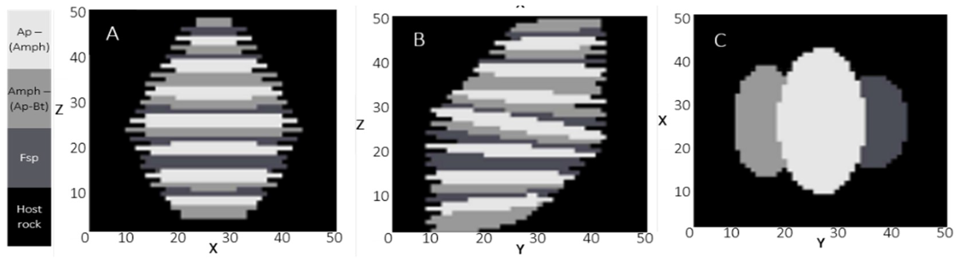
2.2. Synthetic Ore Body Model
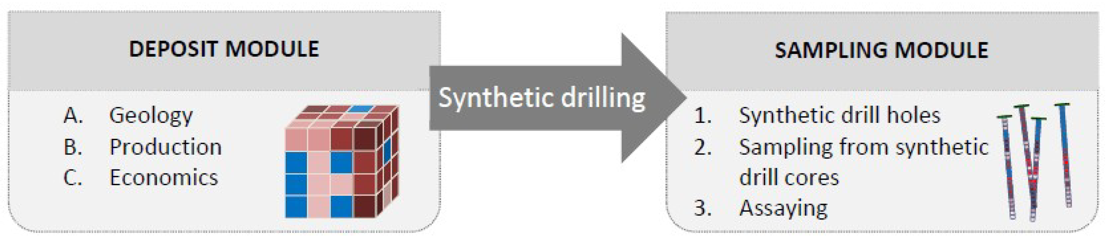
2.3. Synthetic Deposit Module
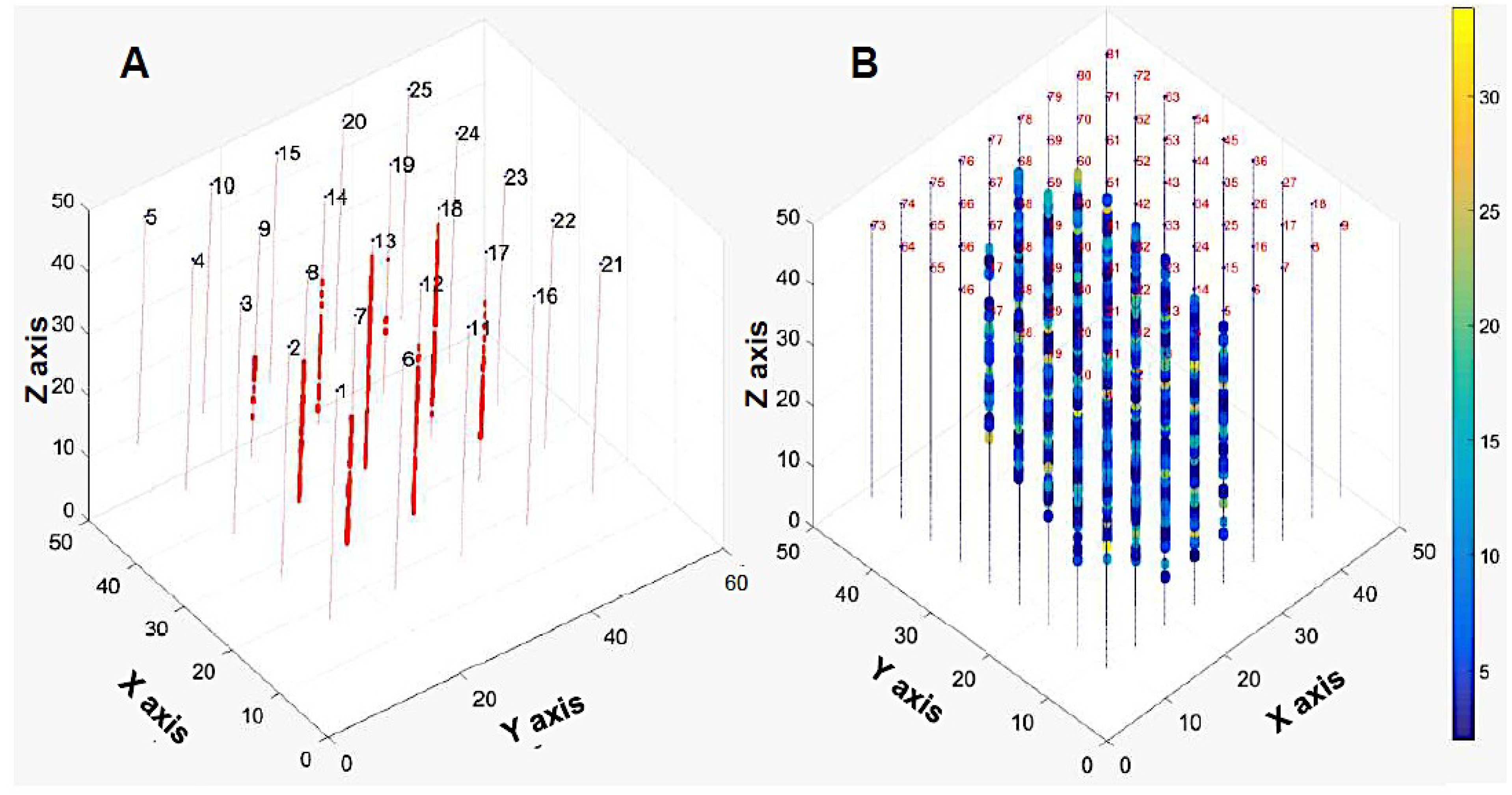
2.3.1. Spatial Data
2.3.2. Database
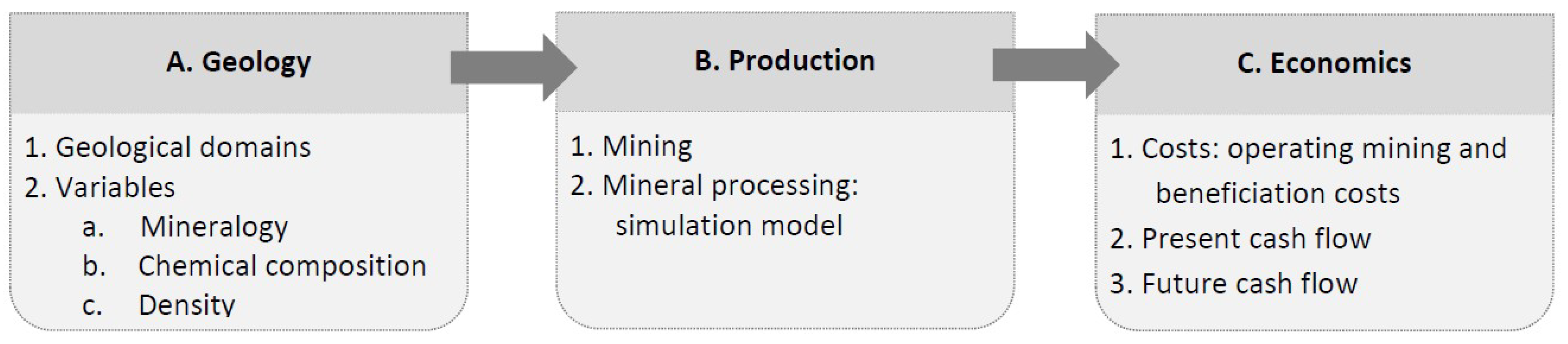
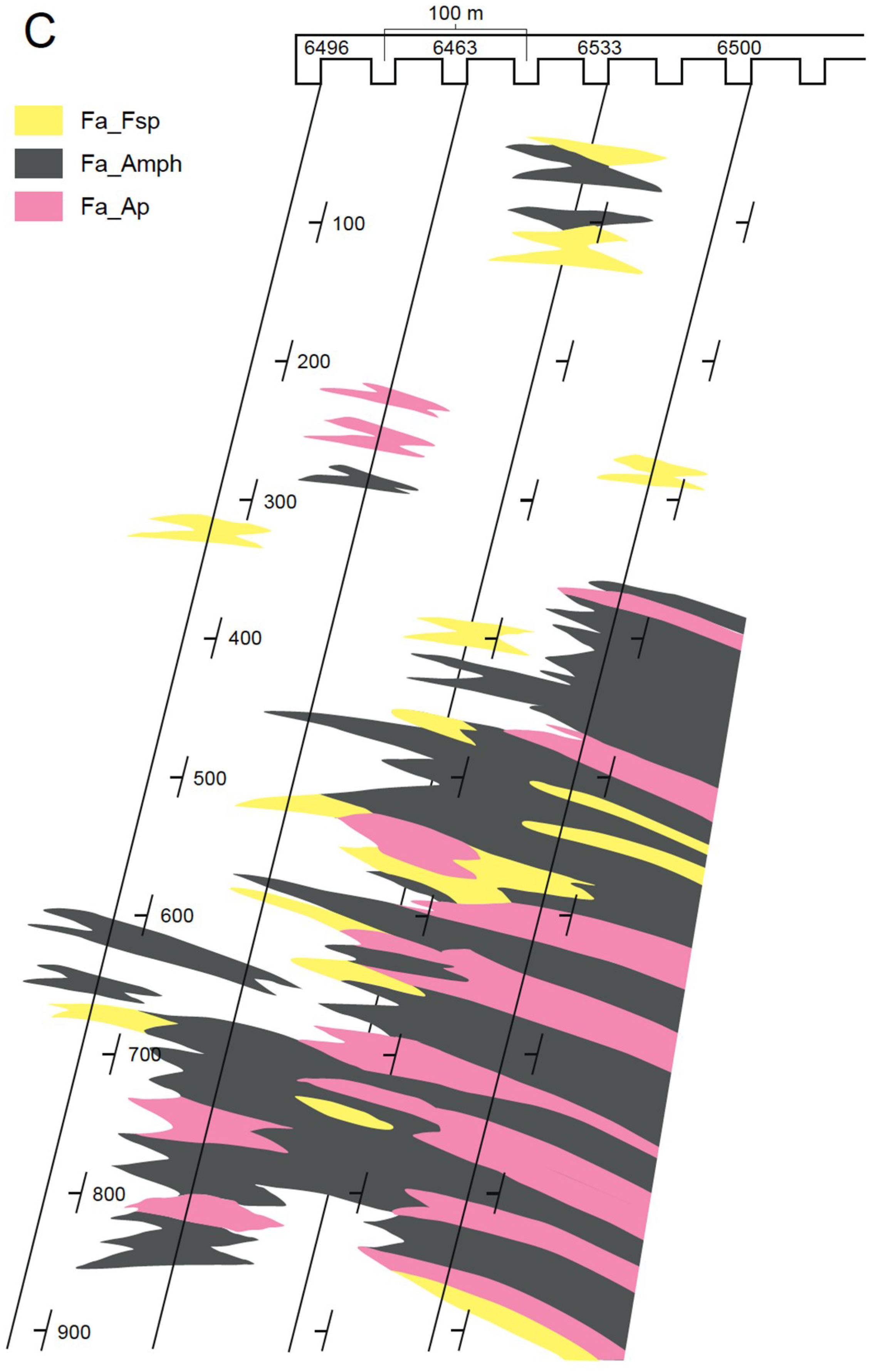
2.3.2.1. Geology
- i
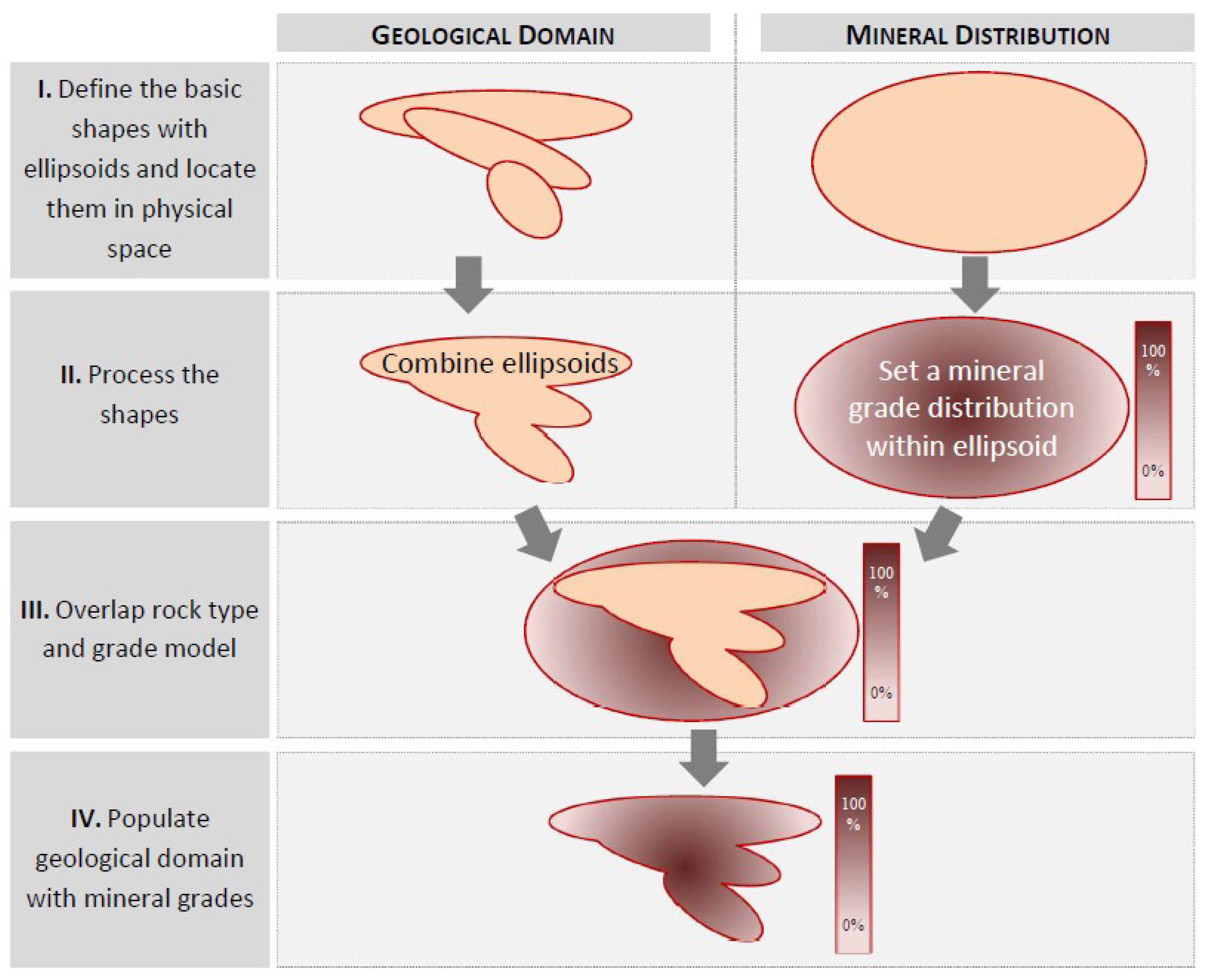
- Stationarity is insured by modelling the “stationarity ellipsoids”. A stationarity ellipsoid is a geometry where the mineral distribution is the same for a given mineral throughout the portion of the voxel model enclosed by this stationarity ellipsoid. The algorithm of describing stationarity ellipsoids is identical to the one used for describing geological domains. Stationarity allow for describing anisotropy of the mineral distributions within the ellipsoids’ dimensions and orientations.
- ii
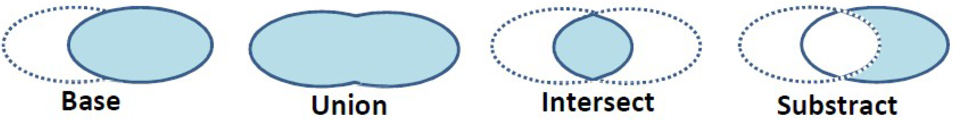
- Spatial conflicts between geological domains and stationarity ellipsoids are resolved with Boolean operations (Figure 4).
- iii
- Minerals modelled with Equations (2)–(4) may have compositions which are outside the normal range of values. Therefore, a certain minimax range can be imposed by rescaling (or truncating) the mineral distribution.
- iv
- The total sum of mineral grades should be closed to 100%. Normalisation of values to a constant sum is also called a closure and forces negative correlations [52,53,54,55,56]. According to Aitchison [57] log-ratios should be used when it is needed to maintain the constant sum constraint. The significance of closure problem for environmental data was emphasised by Filzmoser et al. [58] and Reimann et al. [59], and for compositional geochemical data by Makvandi et al. [60].
2.3.2.2. Production
2.3.2.3. Economics
2.4. Sampling Module
3. How to Use Synthetic Data
3.1. Malmberget Case Study
3.2. Geological Model
3.3. Mining Model
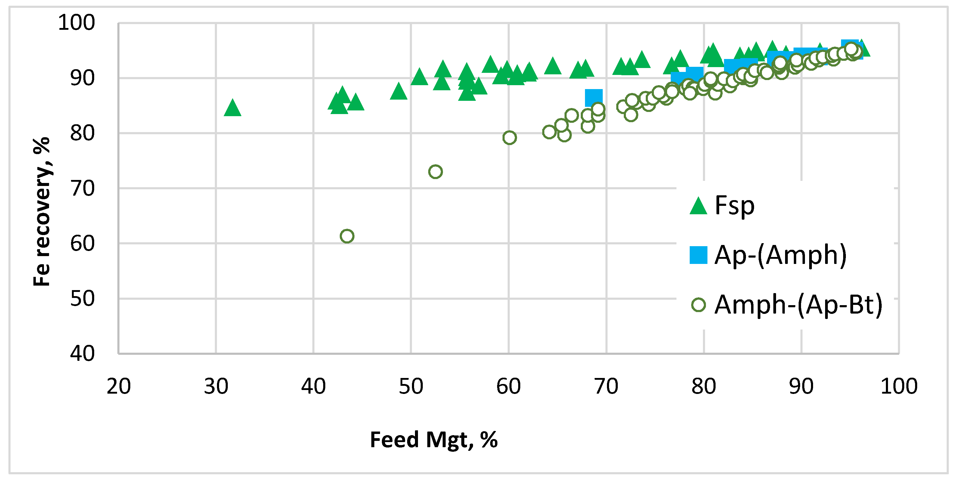
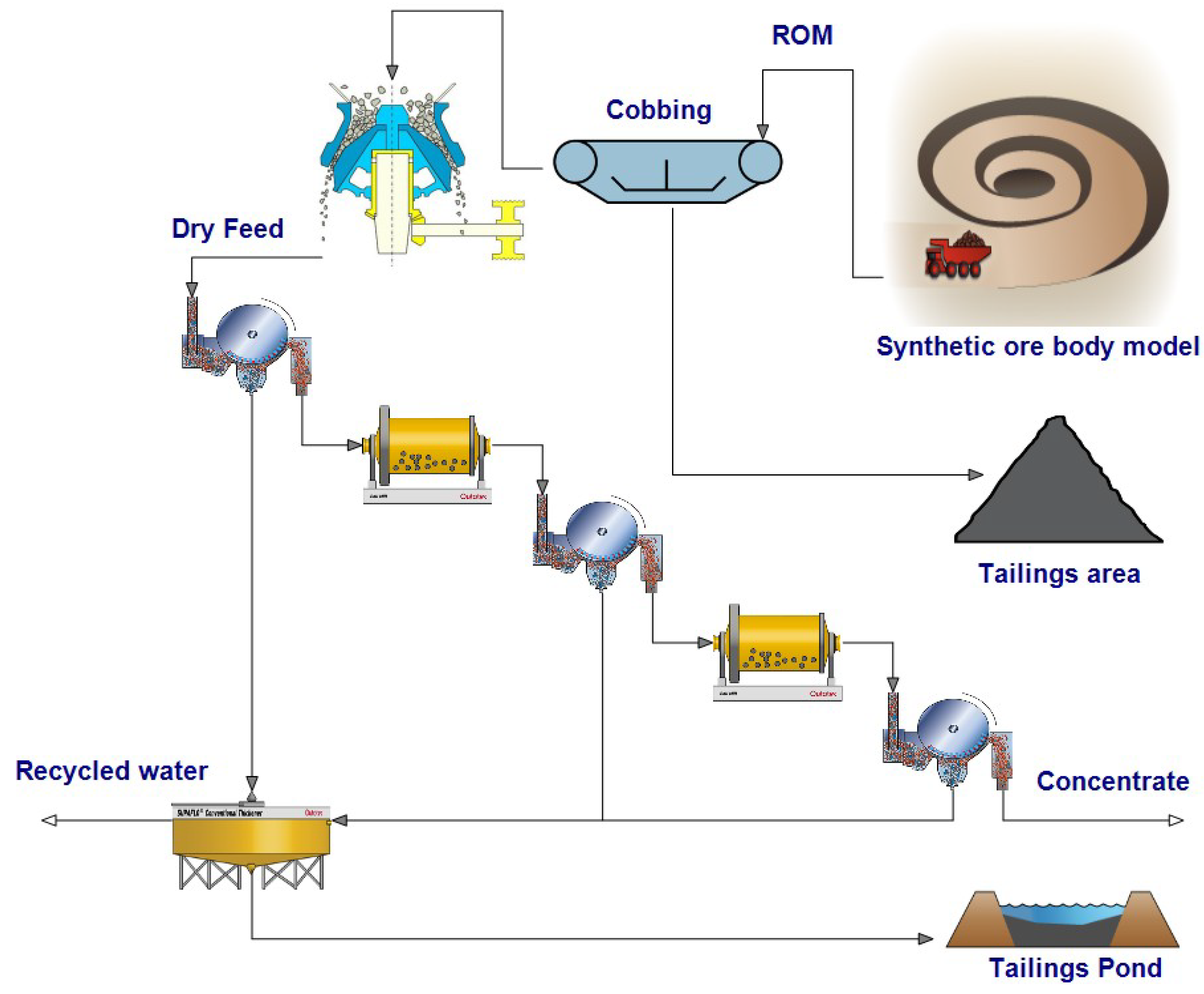
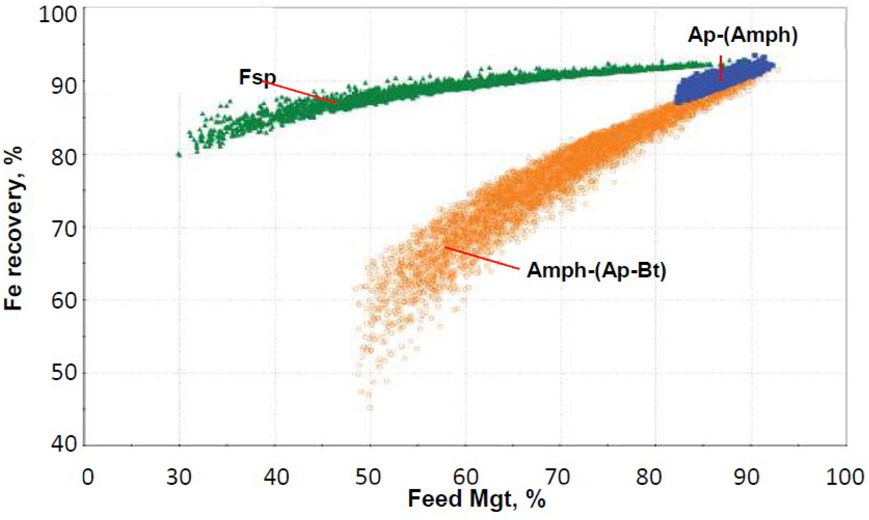
3.4. Process Model
3.5. Synthetic Sampling
4. Implications and Limitations
5. Conclusions
Author Contributions
Funding
Acknowledgments
Conflicts of Interest
References
- Lamberg, P. Particles—The bridge between geology and metallurgy. In Proceedings of the Conference in Minerals Engineering, Luleå, Sweden, 8–9 February 2011; pp. 1–16. [Google Scholar]
- Lund, C.; Lamberg, P. Geometallurgy—A tool for better resource efficiency. Eur. Geol. 2014, 37, 39–43. [Google Scholar]
- Sola, C.; Harbort, G. Geometallurgy—Tricks, traps and treasures. In Proceedings of the 11th AusIMM Mill Operators’ Conference, Hobart, Australia, 29–31 October 2012; pp. 187–196. [Google Scholar]
- Powell, M.S. Utilising orebody knowledge to improve comminution circuit design and energy utilisation. In Proceedings of the Second AUSIMM International Geometallurgy Conference, Brisbane, Australia, 30 September–2 October 2013; pp. 27–35. [Google Scholar]
- Philander, C.; Rozendaal, A. The application of a novel geometallurgical template model to characterise the Namakwa Sands heavy mineral deposit, West Coast of South Africa. Miner. Eng. 2013, 52, 82–94. [Google Scholar] [CrossRef]
- Dunham, S.; Vann, J. Geometallurgy, geostatistics and project value—Does your block model tell you what you need to know? In Proceedings of the Project Evaluation Conference, Melbourne, Australia, 19–20 June 2007; pp. 189–196. [Google Scholar]
- Boogaart, K.G.; van den Tolosana-Delgado, R. Predictive geometallurgy: An interdisciplinary key challenge for mathematical geosciences. In Handbook of Mathematical Geosciences: Fifty Years of IAMG. (Open Access); Daya, B.S., Qiuming, C., Frits, A., Eds.; Springer International Publishing: Cham, Switzerland, 2018; pp. 673–686. [Google Scholar]
- Coward, S.; Vann, J.; Dunham, S.; Stewart, M. The primary-response framework for geometallurgical variables. Seventh International Mining Geology Conference, Perth, WA, Australia, 17–19 August 2009; pp. 109–113. [Google Scholar]
- Tolosana-Delgado, R.; Mueller, U.; Van Boogaart, K.G. Den; Ward, C.; Gutzmer, J. Improving processing by adaption to conditional geostatistical simulation of block compositions. J. S. Afr. Inst. Min. Metall. 2015, 115, 13–26. [Google Scholar] [CrossRef]
- Sepulveda, E.; Dowd, P.A.; Xu, C.; Addo, E. Multivariate modelling of geometallurgical variables by projection pursuit. Math. Geosci. 2016, 121–143. [Google Scholar] [CrossRef]
- Everett, J.E. Simulation to reduce variability in iron ore stockpiles. Math. Comput. Simul. 1997, 4, 563–568. [Google Scholar] [CrossRef]
- Everett, J.E.; Howard, T.J. Predicting finished product properties in the mining industry from pre-extraction data. In the First Ausimm International Geometallurgy Conference, Brisbane, QLD, 5–7 September 2011; Australasian Institute of Mining and Metallurgy (AusIMM): Brisbane, Australia, 2011; pp. 205–215. [Google Scholar]
- Jupp, K.; Howard, T.J.; Everett, J.E. Generating synthetic data for simulation modelling in iron ore. In The Second AUSIMM International Geometallurgy Conference/Brisbane, QLD, 30 September–2 October 2013; Australasian Institute of Mining and Metallurgy (AusIMM): Brisbane, QLD, Australia, 2013; pp. 231–237. [Google Scholar]
- Malmqvist, K.; A Mathematical Study of a Deeper Exploration Project. Description of the Simulation Model and Procedure. Available online: http://umu.diva-portal.org/smash/get/diva2:633654/FULLTEXT02.pdf (accessed on 11 December 2015).
- Malmqvist, K. A Feasibility Study of Exploration for Deep Seated ore Bodies in the Skelefte Field. Ph.D. Thesis, Umeå Universitet, Umeå, Sweden, 1979. [Google Scholar]
- Malmqvist, K.; Malmqvist, L.; Zweifel, H. Computer simulation of exploration for deep-seated orebodies in mining districts. Econ. Geol. 1980, 75, 927–935. [Google Scholar] [CrossRef]
- Chatterjee, S.; Dimitrakopoulos, R. Multi-scale stochastic simulation with a wavelet-based approach. Comput. Geosci. 2012, 45, 177–189. [Google Scholar] [CrossRef]
- Mustapha, H.; Dimitrakopoulos, R. HOSIM: A high-order stochastic simulation algorithm for generating three-dimensional complex geological patterns. Comput. Geosci. 2011, 37, 1242–1253. [Google Scholar] [CrossRef]
- Schouwstra, R.; De Vaux, D.; Muzondo, T.; Prins, C. A geometallurgical approach at Anglo American Platinum’s Mogalakwena operation. In The Second AUSIMM International Geometallurgy Conference/Brisbane, QLD, 30 September–2 October 2013; The Australasian Institute of Mining and Metallurgy (AusIMM): Brisbane, Australia, 2013; pp. 85–92. [Google Scholar]
- Armstrong, B.; Czerw, A.; Glen, J.; Johnson, N.W.; Munro, P.D. Realisation of value through identification of various oxidation fronts and mineralisation styles at Trilogy Cu-Au-Ag-Pb-Zn deposit. In Proceedings of the First AUSIMM International Geometallurgy Conference, Brisbane, Australia, 5–7 September 2011; pp. 47–51. [Google Scholar]
- Gilardi, N. Machine learning for automatic environmental mapping: When and how. In Report: Automatic Mapping Algorithms for Routine and Emergency monitoring Data; Dubois, G., Ed.; European Commission: Luxembourg, Germany, 2005; pp. 123–137. [Google Scholar]
- Hengl, T. A Practical guide to Geostatistical Mapping. Sci. Tech. Res. Ser. 2009, 271. [Google Scholar] [CrossRef]
- Chilès, J.-P.; Delfiner, P. Geostatistics: Modeling Spatial Uncertainty, 2nd ed.; Balding, D.J., Cressie, N.A.C., Fitzmaurice, G.M., Goldstein, H., Johnstone, I.M., Molenberghs, G., Scott, D.W., Smith, A.F.M., Tsay, R.S., Eds.; John Wiley & Sons, Inc: Hoboken, NJ, USA, 2012; ISBN 978-0-87-421656-1. [Google Scholar]
- Mariethoz, G.; Caers, J. Multiple-Point Geostatistics: Stochastic Modeling with Training Images; John Wiley & Sons, Ltd.: Chichester, UK, 2015; ISBN 978-1-118-66275-5. [Google Scholar]
- Michael, H.A.; Li, H.; Boucher, A.; Sun, T.; Caers, J.; Gorelick, S.M. Combining geologic-process models and geostatistics for conditional simulation of 3-D subsurface heterogeneity. Water Resour. Res. 2010, 46. [Google Scholar] [CrossRef]
- Sarma, D.D. Geostatistics with applications in earth sciences. Geostat. Appl. Earth Sci. 2009, 1–205. [Google Scholar] [CrossRef]
- Isaaks, E.H.; Srivastava, R.M. Applied Geostatistics; Oxford University Press: New York, NY, USA, 1989; ISBN 0195050134. [Google Scholar]
- Gandhi, S.M.; Sarkar, B.C. Essentials of Mineral Exploration and Evaluation; Elsevier: Amsterdam, The Netherlands, 2016; ISBN 978-0-12-805329-4. [Google Scholar]
- Matheron, G. Principles of geostatistics. Econ. Geol. 1963, 58, 1246–1266. [Google Scholar] [CrossRef]
- Remy, N.; Boucher, A.; Wu, J. Applied Geostatistics with SGeMS: A User’s Guide; Cambridge University Press: Cambridge, UK, 2009; ISBN 0521514142. [Google Scholar]
- Koltermann, C.E.; Gorelick, S.M. Heterogeneity in sedimentary deposits: A review of structure-imitating, process-imitating, and descriptive approaches. Water Resour. Res. 1996, 32, 2617–2658. [Google Scholar] [CrossRef]
- Smith, M.J.; Goodchild, M.F.; Longley, P.A. Geospatial Analysis: A Comprehensive Guide to Principles Techniques and Software Tools, 6th ed.; Winchelsea Press: Winchelsea, UK, 2018; ISBN 978-1-91-255603-8. [Google Scholar]
- Watkins, A.E.; Scheaffer, R.L.; Cobb, G.W. Statistics in Action: Understanding a World of Data, 2nd ed.; Key Curriculum Press: Emeryville, CA, USA, 2008; ISBN 978-1-55-953909-8. [Google Scholar]
- Eriksson, L.; Byrne, T.; Johansson, E.; Trygg, J.; Vikström, C. Multi- and Megavariate Data Analysis: Basic Principles and Applications, 3rd ed.; Umetrics Academy: Umeå, Sweden, 2013; ISBN 10. [Google Scholar]
- Suthaharan, S. Machine Learning Models and Algorithms for Big Data Classification: Thinking with Examples for Effective Learning; Springer: Greensboro, NC, USA, 2016; ISBN 978-1-4899-7640-6. [Google Scholar]
- Aggarwal, C.C. Data Classification Algorithms and Applications, 1st ed.; Chapman and Hall/CRC: New York, NY, USA, 2014; ISBN 978-8-57-811079-6. [Google Scholar]
- Frank, E.; Hall, M.A.; Witten, I.H. The WEKA Workbench, 4th ed.; Morgan Kaufmann: San Francisco, CA, USA, 2016; pp. 553–571. [Google Scholar] [CrossRef]
- Outotec HSC Chemistry 7.1—Chemical Reaction and Equilibrium Software with Thermochemical Database and Simulation Module 2012. Available online: https://www.outotec.com/products/digital-solutions/hsc-chemistry/ (accessed on 16 November 2018).
- Mcinnes, C.; Dobby, G.; Schaffer, M. The Application of CEET and FLEET in the Base Metals Industry: Current Status and Future Vision. Available online: http://www.sgs.com/minerals. (accessed on 16 November 2018).
- Cycad Process—Official Website Cycad Process—Simulation Software for the Metallurgical Industry. Available online: http://www.cycadprocess.com/about-cycad-process (accessed on 4 April 2016).
- FLSmidth—Official Website Process Training Simulation—Advanced Environment for Training of Process Operators. Available online: http://www.flsmidth.com/en-US/Industries/Categories/Products/Electrical+and+Automation/Process+Automation/Process+Simulation/Cemulator (accessed on 4 April 2016).
- ANDRITZ—Official Website IDEAS Simulation Software. Available online: http://www.andritz.com/products-and-services/pf-detail.htm?productid=18154 (accessed on 27 March 2016).
- Ziemski, M.; Bye, A.; Plint, N.; Cole, M.; Tordoir, A. An integrated geology-mine-plant and eco-efficiency simulator for Anglo Platinum’s evaluation and operational improvement initiatives. In Proceedings of the XXV International Mineral Processing Congress (IMPC) 2010, Brisbane, Australia, 6–10 September 2010; pp. 3629–3638. [Google Scholar]
- Suthers, S.P.; Clout, J.M.F.; Donskoi, E. Prediction of plant process performance using feed characterisation—An emerging tool for plant design and optimisation. In Proceedings of the MetPlant, Perth, Australia, 6–7 September 2004; pp. 203–217. [Google Scholar]
- Herbst, J.A.; Pate, W.T. Dynamic simulation of size reduction operations from Mine-to-Mill. In Proceedings of the Mine to Mill: Exploring the Relationship between Mining and Mineral Processing, Brisbane, Australia, 11–14 October 1998; pp. 243–248. [Google Scholar]
- King, R.P. Modeling and Simulation of Mineral Processing Systems, 1st ed.; Reed Educational and Professional Publishing Ltd.: Woburn, MA, USA, 2001; ISBN 0-7506-4884-8. [Google Scholar]
- Schneider Electric DYNSIM. High Fidelity Dynamic Operator Training Solutions. Available online: http://software.schneider-electric.com/ (accessed on 4 April 2016).
- Sanchidrián, J.A.; Ouchterlony, F.; Moser, P.; Segarra, P.; López, L.M. Performance of some distributions to describe rock fragmentation data. Int. J. Rock Mech. Min. Sci. 2012, 53, 18–31. [Google Scholar] [CrossRef]
- David, D. The importance of geometallurgical analysis in plant study, design and operational phases. In Proceedings of the 9th Mill Operators’ Conference, Fremantle, Australia, 19–21 March 2007; pp. 241–247. [Google Scholar]
- Maptek Vulcan 10.1.4. Available online: http://www.maptek.com/ (accessed on 19 February 2018).
- Dassault Systems Geovia Surpac. Available online: https://www.3ds.com/ (accessed on 19 February 2018).
- Pawlowsky-Glahn, V.; Egozcue, J.J. The closure problem: One hundred years of debate. In Proceedings of the Mining Příbram Symposium. Section: Mathematical Methods in Geology, Prague, Czech Republic, 10–14 October 2011; p. 8. [Google Scholar]
- Chayes, F. On correlation between variables of constant sum. J. Geophys. Res. 1960, 65, 4185–4193. [Google Scholar] [CrossRef]
- Pawlowsky-Glahn, V.; Egozcue, J.J. Spatial analysis of compositional data: A historical review. J. Geochem. Explor. 2016, 164, 28–32. [Google Scholar] [CrossRef]
- Butler, J.C. Closure and Ratio Correlation Analysis of Lunar Chemical and Grain Size Data (Report# NASA-CR-153063); University of Houston: Houston, TX, USA, 1976. [Google Scholar]
- Aitchison, J.; Egozcue, J.J. Compositional data analysis: Where are we and where should we be heading? Math. Geol. 2005, 829–850. [Google Scholar] [CrossRef]
- Aitchison, J. The Statistical Analysis of Compositional Data; Chapman and Hall, London.: London, UK, 1986; ISBN 978-9-40-108324-9. [Google Scholar]
- Filzmoser, P.; Hron, K.; Reimann, C. Univariate statistical analysis of environmental (compositional) data: Problems and possibilities. Sci. Total Environ. 2009, 407, 6100–6108. [Google Scholar] [CrossRef] [PubMed]
- Reimann, C.; Filzmoser, P.; Fabian, K.; Hron, K.; Birke, M.; Demetriades, A.; Dinelli, E.; Ladenberger, A. The concept of compositional data analysis in practice—Total major element concentrations in agricultural and grazing land soils of Europe. Sci. Total Environ. 2012, 426, 196–210. [Google Scholar] [CrossRef] [PubMed]
- Makvandi, S.; Ghasemzadeh-Barvarz, M.; Beaudoin, G.; Grunsky, E.C.; Beth McClenaghan, M.; Duchesne, C. Principal component analysis of magnetite composition from volcanogenic massive sulfide deposits: Case studies from the Izok Lake (Nunavut, Canada) and Halfmile Lake (New Brunswick, Canada) deposits. Ore Geol. Rev. 2016, 72, 60–85. [Google Scholar] [CrossRef]
- Laurich, R. 5.2 Ultimate Pit Definition. In Surface Mining, 2nd ed.; Kennedy, A., Ed.; Society for Mining, Metallurgy, and Exploration, Inc. (SME): Littleton, CO, USA, 1990; p. 1206. ISBN 978-0-87335-102-7. [Google Scholar]
- Lerchs, H.; Grossmann, I.F. Optimum design of open pit mines. Can. Inst. Min. Metall. Bull. 1965, 58, 47–54. [Google Scholar]
- Picard, J.-C. Maximal closure of a graph and applications to combinatorial problems. Manag. Sci. 1976, 22, 1268–1272. [Google Scholar] [CrossRef]
- Dagdelen, K.; Johnson, T.B. Optimum open pit mine production scheduling by lagrangian parametrization. In Proceedings of the APCOM’86 Application of Computers and Operations Research in the Mineral Industry, Littleton, CO, USA, 14–18 April 1986; pp. 127–142. [Google Scholar]
- Newman, A.M.; Rubio, E.; Caro, R.; Weintraub, A.; Eurek, K. A review of operations research in mine planning. Interfaces 2010, 40, 222–245. [Google Scholar] [CrossRef]
- Meagher, C.; Dimitrakopoulos, R.; Avis, D. Optimized open pit mine design, pushbacks and the gap problem—A review. J. Min. Sci. 2014, 50, 508–526. [Google Scholar] [CrossRef]
- Lamberg, P.; Lund, C. Taking liberation information into a geometallurgical model-case study Malmberget, Northern Sweden. In Proceedings of the Process Mineralogy’12, Cape Town, South Africa, 7–9 November 2012. [Google Scholar]
- Lamberg, P.; Vianna, S. A technique for tracking multiphase mineral particles in flotation circuits. Meeting of the Southern Hemisphere on Mineral Technology: 20/11/2007-24/11/2007, Ouro Preto, Portugal, 20–24 November 2007. [Google Scholar]
- Koch, P.-H.; Rosenkranz, J. Texture-based liberation models for comminution. In Proceedings of the Konferens i Mineralteknik 2017, Lulea, Sweden, 7–8 February 2017; pp. 83–96. [Google Scholar]
- Lund, C.; Lamberg, P.; Lindberg, T. Development of a geometallurgical framework to quantify mineral textures for process prediction. Miner. Eng. 2015, 82, 61–77. [Google Scholar] [CrossRef]
- Lamberg, P. Structure of a property based simulator for minerals and metallurgical industry. In Proceedings of the SIMS 2010, The 51st Conference on Simulation and Modelling, Oulu, Finland, 14–15 October 2010; p. 5. [Google Scholar]
- Ouchterlony, F. The Swebrec© function: Linking fragmentation by blasting and crushing. Min. Technol. 2005, 114, 29–44. [Google Scholar] [CrossRef]
- InfoMine Mining Cost Models: Mine & Mill Cost Models, Mining Taxes, Metal Prices, Smelting, Equipment, Supplies, Transportation, Utility and Labor Costs. Available online: http://costs.infomine.com (accessed on 19 February 2018).
- Sayadi, A.R.; Khalesi, M.R.; Borji, M.K. A parametric cost model for mineral grinding mills. Miner. Eng. 2014, 55, 96–102. [Google Scholar] [CrossRef]
- Kitco Metalc Inc. Available online: http://www.kitco.com/ (accessed on 15 May 2017).
- LME London Metal Exchange. Available online: https://www.lme.com/ (accessed on 19 February 2018).
- Darling, P. SME Mining Engineering Handbook; Darling, P., Ed.; Society for Mining, Metallurgy, and Exploration, Inc. (SME): Littleton, CO, USA, 2011; Volume 66, ISBN 978-0873352642. [Google Scholar]
- Lund, C.; Lamberg, P.; Lindberg, T. Practical way to quantify minerals from chemical assays at Malmberget iron ore operations—An important tool for the geometallurgical program. Miner. Eng. 2013, 49, 7–16. [Google Scholar] [CrossRef]
- Bauer, T.E.; Andersson, J.B.H.; Sarlus, Z.; Lund, C.; Kearney, T. Structural controls on the setting, shape, and hydrothermal alteration of the Malmberget iron oxide-apatite deposit, Northern Sweden. Econ. Geol. 2018, 113, 377–395. [Google Scholar] [CrossRef]
- Lund, C. Mineralogical, Chemical and Textural Characterisation of the Malmberget Iron Ore Deposit for a Geometallurgical Model. Doctoral Thesis, Luleå University of Technology, Luleå, Sweden, 2013. [Google Scholar]
- Koch, P.-H.; Lamberg, P.; Rosenkranz, J. How to build a process model in a geometallurgical program? In Proceedings of the 13th Biennial SGA Meeting, Nancy, France, 24–27 August 2015; 2015; pp. 1419–1422. [Google Scholar]


| Classification of the Methods | References | Number of Data Points | Smoothing | Realism | ||
|---|---|---|---|---|---|---|
| Geostatistics | Estimations (e.g., univariate, indicator, co-, and block kriging) | [23,24,26,27,28,29] | Large | High | Low/Medium | |
| Simulations | Stochastic (e.g., LU, sequential Gaussian, and Block Error simulations) | [23,24,30] | Medium | Low | Medium/High | |
| Process (e.g., process based, process-mimicking) | [24,31] | Small | Low | High | ||
| Non-geostatistics | Statistics | Uni-, Bivariate (e.g., Inverse distance weighting, nearest neighbour, polynomial regression, splines) | [32,33] | Medium/Large | High | Low |
| Multivariate (e.g., K-means clustering, PLS regression) | [34] | Medium/Large | Medium | Medium | ||
| Machine learning | Unsupervised: clustering (e.g., K-means) | [35,36,37] | Medium | Medium | Medium | |
| Supervised: regression (e.g., Neural networks) and classification (e.g., nearest neighbours, decision trees) | Large | Medium | Medium/High | |||
| Mining Method | Relative Cost | Flexibility | Selectivity | Recovery, % | Dilution, % |
|---|---|---|---|---|---|
| Surface mining | 0.10 | moderate | moderate | High | Low |
| Room-and-pillar (coal) | 0.30 | high | high | 50–80 | 20 |
| Stope-and-pillar | 0.30 | high | high | 75 | 15 |
| Sublevel caving | 0.40 | low | low | 75 | 15 |
| Shrinkage stopping | 0.50 | moderate | moderate | 80 | 10 |
| Cut-and-fill | 0.60 | moderate | high | 100 | 0 |
| Timbered square set | 1.00 | moderate | high | 100 | 0 |
| Longwall | 0.20 | low | low | 80 | 10 |
| Sublevel caving (top slicing) | 0.50 | low | low | 90 | 20 |
| Block caving | 0.20 | low | low | 90 | 20 |
| Step1 | → | Step 2 | → | Step3 | |||||||||||||||||
| Ore classification (Qualitative) | Geological model (Quantitative) | Process model (Cobbing concentrate) | |||||||||||||||||||
| Ore Type | Main Associating Minerals | Textural Type Name | Modal Composition (Average Bulk), wt.% | Liberation Distribution of Mgt, (Average Bulk), % | Grade, % | Recovery, % | |||||||||||||||
| Mgt | Ab | Act | Ap | Bt | Liberated | Ab | Act | Ap | Bt | Fe/SiO2 | Fe | ||||||||||
| Semi massive | Ab, Qtz, Bt, Amph | Fsp | 55.1 | 35.0 | 7.6 | 0.4 | 1.8 | 95.9 | 2.2 | 1.1 | 0.5 | 0.4 | 68.2/2.7 | 93.6 | |||||||
| Massive | Amph | Amph-(Ap, Bt) | 66.4 | 2.9 | 23.0 | 1.3 | 6.4 | 94.5 | 0.5 | 3.8 | 0.4 | 0.8 | 64.3/5.2 | 88.8 | |||||||
| Ap, Amph | Ap – (Amph) | 86.6 | 0.1 | 3.3 | 7.1 | 2.8 | 89.2 | 0.8 | 0.9 | 6.0 | 3.0 | 66.0/4.1 | 90.0 | ||||||||
| Element | Fe | Ti | V | Si | Al | Ca | Mg | Na | K | P |
|---|---|---|---|---|---|---|---|---|---|---|
| RSD | 0.1 | 1.0 | 1.4 | 1.0 | 2.0 | 3.2 | 2.8 | 2.0 | 2.4 | 0.7 |
| Metrics | Modal Mineralogy, % | Elemental Composition, % (*—ppm) | |||||||||||||
|---|---|---|---|---|---|---|---|---|---|---|---|---|---|---|---|
| Mgt | Ab | Bt | Act | Ap | Fe | Ti * | V * | Si | Al | Ca | Mg | Na | K | P | |
| Average | 98.1 | 0.2 | 0.3 | 0.5 | 0.5 | 71.4 | 100 | 299.9 | 0.2 | 0.1 | 0.2 | 0.1 | 0 | 0 | 0.1 |
| Min | 91.2 | 0 | 0.1 | 0 | 0 | 66.5 | 100 | 200 | 0.1 | 0.1 | 0 | 0.1 | 0 | 0 | 0 |
| Max | 99.4 | 0.7 | 1.2 | 2 | 5.8 | 72.3 | 100 | 300 | 0.7 | 0.2 | 2.5 | 0.4 | 0.1 | 0.1 | 0.9 |
| Stdev | 0.8 | 0.1 | 0.1 | 0.4 | 0.4 | 0.6 | 0 | 1.6 | 0.1 | 0 | 0.2 | 0.1 | 0 | 0 | 0.1 |
| Skewness | −1.8 | 1.5 | 1.2 | 1.3 | 2.3 | −1.8 | −1 | −62.6 | 1.2 | 0.9 | 2.2 | 1.3 | 1 | 1 | 2.2 |
| Kurtosis | 8 | 5.1 | 4.8 | 3.7 | 15.1 | 8.4 | −2 | 3884.3 | 3.8 | 3.5 | 14.2 | 4.1 | 3.8 | 4.2 | 14.9 |
© 2018 by the authors. Licensee MDPI, Basel, Switzerland. This article is an open access article distributed under the terms and conditions of the Creative Commons Attribution (CC BY) license (http://creativecommons.org/licenses/by/4.0/).
Share and Cite
Lishchuk, V.; Lund, C.; Lamberg, P.; Miroshnikova, E. Simulation of a Mining Value Chain with a Synthetic Ore Body Model: Iron Ore Example. Minerals 2018, 8, 536. https://doi.org/10.3390/min8110536
Lishchuk V, Lund C, Lamberg P, Miroshnikova E. Simulation of a Mining Value Chain with a Synthetic Ore Body Model: Iron Ore Example. Minerals. 2018; 8(11):536. https://doi.org/10.3390/min8110536
Chicago/Turabian StyleLishchuk, Viktor, Cecilia Lund, Pertti Lamberg, and Elena Miroshnikova. 2018. "Simulation of a Mining Value Chain with a Synthetic Ore Body Model: Iron Ore Example" Minerals 8, no. 11: 536. https://doi.org/10.3390/min8110536
APA StyleLishchuk, V., Lund, C., Lamberg, P., & Miroshnikova, E. (2018). Simulation of a Mining Value Chain with a Synthetic Ore Body Model: Iron Ore Example. Minerals, 8(11), 536. https://doi.org/10.3390/min8110536