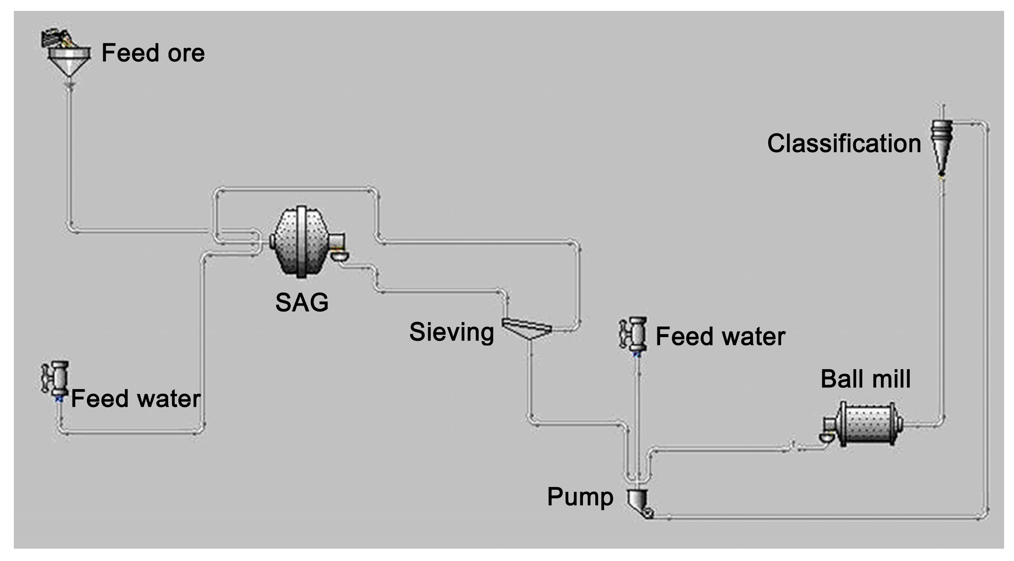
3.5.1. Establishment of SAG-Ball Mill Circuit
Figure 5 shows the well-established model for a closed-circuit SAG-ball mill using JKSimMet. Apart from the primary parts of the circuit, such as the SAG mill, sieving, ball mill, and hydrocyclone, two water supply modules have been included to adjust the grinding concentration in the SAG mill,
i.e., the percentage solids in the feed, and the feed solids for the hydrocyclone, respectively.
A SAG mill module with a variable speed and a fully mixed ball mill module were selected in the modelling process, with these two modules being able to be enlarged. Standard efficiency curve models were chosen for sieving and cyclone classification. Considering the grinding procedure, the annual handling capacity and the total working time in the grinding and separation sections, the production capacity was calculated as 631.3 t/h. Hence, a feed rate of 635 t/h was selected.
The ore that was directly obtained from underground was coarsely crushed to < 250 mm, which was then transported to the grinding mill. If the size of the output of the coarse crusher (S) was 150 mm, the
F80 was calculated to be approximately 111.1 mm (0.2·S·(
DWi)
0.7) and 107.5 mm (S-78.7-28.4·ln(
ta)), respectively, according to the JKSimMet model. Therefore, a
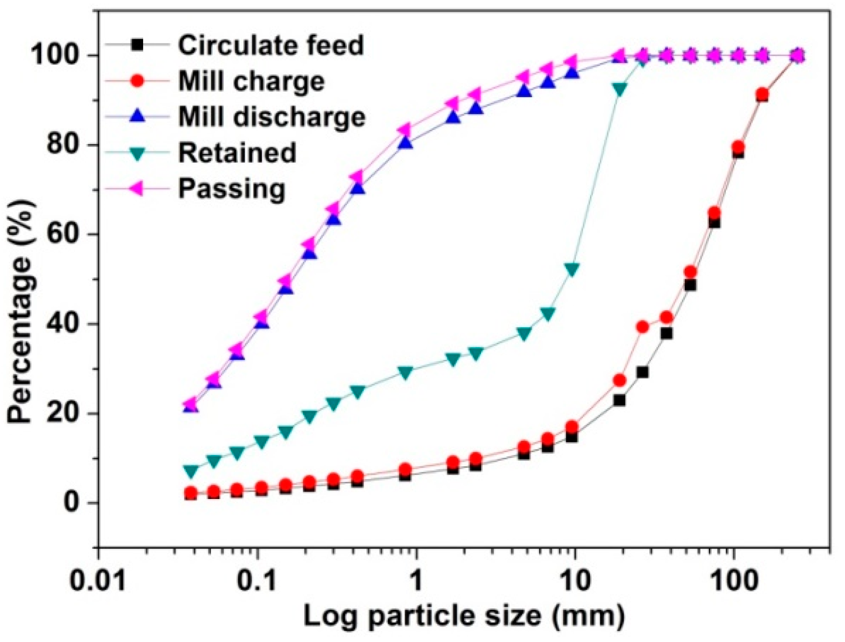
F80 value of 110 mm was chosen for closed circuit testing, with the size distribution from this circuit being shown in
Figure 6.
A SAG mill with a diameter of 10.67 m and a length of 5.33 m was initially selected for the grinding circuit. It should be noted that the diameter and length chosen are the inner dimensions of the SAG mill. Other parameters such as 74% of the desired speed, 8% ball charge, maximum diameter of steel balls of 120 mm, grinding concentration of 75%, grid size of 20 mm, and sieve size of 12 mm (d50c = 11 mm) were selected as well. These parameters were initially applied to simulate the steady state process for the SAG circuit. The modelling was conducted based on progressively adjusting parameters until satisfactory results were obtained, e.g., a SAG mill with a mill charge of 25% solids and a cycling charge less than 25%.
Table 5 shows the progress of adjusting parameters and the results derived from modelling. It was found that the initially selected SAG mills (Φ10.67 m × 5.33 m and Φ10.36 m × 5.18 m) were too big as the mill charges were 21.81% and 23.42%, respectively, in the first two modellings. The third SAG mill option with a size of Φ10.06 m × 5.03 m was quite suitable as the mill charging was 25.25% with a cycling charge of 6.17%. It should be noted that optimizing the mill charge can be further improved by adjusting other parameters such as increasing the ball charge to 8.5% to obtain a mill charge of less than 25% (the fourth simulation shown in
Table 5). Therefore, a SAG mill (Φ10.06 m × 5.03 m) with a driving power of 7321 kW was finally selected, while the related specific energy consumption was calculated as 11.53 kWh/t.
Table 6 shows the modelling results for SAG circuit based on the selected parameters described above, giving a product with a
P80 value of 0.651 mm and 34.12% of final particles smaller than 0.074 mm.
3.5.2. Selection of Ball Mill
The product from the SAG circuit (
Section 3.5.1) was used as the feed to the ball mill circuit. An overflow ball mill with a diameter of 5.03 m and a length of 8.84 m was initially selected for the modelling. The operation parameters were set as follows: 73% of the desired speed, 38% ball charge, a maximum diameter of 80 mm for the steel balls, and a solids concentration of 60% for the hydrocyclone,
d50c = 0.150 mm. Similar to the SAG circuit simulation, a steady state process was simulated for the ball mill circuit with the requirements of a cycling charge of around 250% and less than 60% of the final product with a size of −0.074 mm,
etc. The simulation process and results are shown in
Table 7. It is evident that the initial selection of a ball mill size of Φ5.03 m × 8.84 m produced 61.62% −0.074 mm materials, but the cycling charge was only 240.9%, indicating this size was too big. A slight improvement was observed for the second ball mill (Φ5.03 m × 8.53 m), while the third option (Φ5.03 m × 8.23 m) seemed to meet the requirements. With slight adjustments in hydrocyclone solids concentration and
d50c in the fourth and fifth simulations, respectively, a mill power of 3767 kW and a cycling charge of 252.4% were obtained. The
P80 of the final product was observed to be 0.137 mm, while the specific energy consumption was calculated as 5.93 kWh/t.
3.5.3. Comparison of Comminution Circuits
The basic data used in the Morrell model were obtained from the SMC and Bond ball work index tests and the specific energy consumptions of the jaw crusher and ball mill circuits were calculated using Equations (5)–(8):
where
K1 is 1.0 for all circuits that do not contain a recycle pebble crusher and 0.95 where circuits do have a pebble crusher,
x1 is the
P80 (µm) of the product of the last stage of crushing before grinding,
x2 is 750 µm, and
Mia is the coarse ore work index and provided directly by the SMC Test.
where
x2 is 750 µm,
x3 is the
P80 (µm) of final grind, and
Mib is provided by data from the standard Bond ball mill work index test.
where
K2 is 1.0 for all crushers operating in a closed circuit with a classifying screen. If the crusher is in an open circuit, e.g., a pebble crusher in a AG/SAG circuit,
K2 takes the value of 1.19,
x1 is the
P80 (µm) of the circuit feed,
x2 is the
P80 (µm) of the circuit product, and
Mic is the coarse ore work index and provided directly by the SMC Test.
where
K3 is 0.19,
x1 is the
P80 (µm) of the circuit feed,
x2 is the
P80 (µm) of the circuit product, and
Mia is the coarse ore work index and provided directly by the SMC Test.
The specific energy consumptions of the jaw crusher, HPGR and ball mill circuits were calculated using Equations (9)–(12).
K4 is 1.0 for all HPGRs operating in closed circuit with a classifying screen. If the HPGR is in open circuit,
K4 takes the value of 1.19,
x1 is the
P80 (µm) of the circuit feed,
x2 is the
P80 (µm) of the circuit product, and
Mih is the HPGR ore work index and provided directly by the SMC Test.
The specific energy consumptions of the SAG and ball mill circuits were calculated using Equations (13) and (14).
All these specific energy consumptions of the three combined circuits are shown in
Table 8.
According to the calculation shown above, the specific energy consumption of the second pathway, i.e., jaw crusher + HPGR mill + ball mill, was 1 kWh/t lower than that of the jaw crusher + ball mill option, with the SAG mill + ball mill option being the highest in specific energy consumption.
It should be noted that the specific energy consumption of comminution is the “net energy consumed” in comminuting ores. Some other energies consumed were not considered, e.g., the driving force for the trunnion when using a tumbling mill, the shaft power for the HPGR mill, and the balance between the motor power and no-load power for the jaw crusher. Assuming that the energy loss between the motor and the transmitted power is 6.5% for the tumbling mill, it is estimated that the “gross energy consumption” related to the motor input power was 13.52 kWh/t, which is relatively lower than the 17.46 kWh/t estimated by the JKSimMet model.
The specific energy consumption estimated by the Morrell model was only based on several material characteristics, however, the variation in parameters and technical processes were not considered. In addition, the energy saved in the discarding of coarse particles was not taken into account. These factors will be further investigated in future studies.


