1. Introduction
Gold remains among the most economically significant mineral commodities, yet global discovery rates have declined steadily as near-surface deposits become exhausted [
1]. This trend intensifies demand for systematic, data-driven approaches capable of identifying buried mineralization beneath cover [
2]. Since the late 1950s, quantitative methods—from multivariate statistics [
3,
4] to geographic information system (GIS)-based spatial modeling [
2,
5]—have progressively improved the objectivity and rigor of mineral exploration targeting.
Mineral prospectivity mapping (MPM) leverages spatial statistical models to delineate areas favorable for mineral deposits [
6,
7]. Two broad categories dominate the field: knowledge-driven models, which rely on expert geological interpretation, mineral-systems reasoning, and techniques such as fuzzy logic [
5,
8,
9,
10,
11,
12], and data-driven models, which use training data from known deposits to identify spatial patterns [
13,
14]. Data-driven approaches—including neural networks [
15], random forests [
14], support vector machines [
14], and weights-of-evidence (WoE) [
2,
16]—have gained prominence for their objectivity and reproducibility. More recently, deep learning and Siamese network architectures have been applied to MPM with promising results [
17,
18].
Among data-driven methods, the WoE approach [
2] is particularly well suited for mineral exploration because it is transparent, statistically rigorous, and applicable to small training datasets. Unlike machine-learning black-box models, WoE generates interpretable evidence weights that geologists can evaluate against their domain knowledge [
7,
8]. Moreover, WoE has been successfully integrated with logistic regression [
16] and multi-criteria decision frameworks [
19] to enhance predictive performance.
The Yilgarn Craton of Western Australia hosts world-class orogenic gold deposits within Archean greenstone belts [
20,
21]. Statewide geological and geophysical coverage makes the craton suitable for evaluating a reproducible regional workflow, while the Southern Cross Domain and the Marda-Diemals Greenstone Belt provide the project-scale geological context for subsequent interpretation [
22,
23].
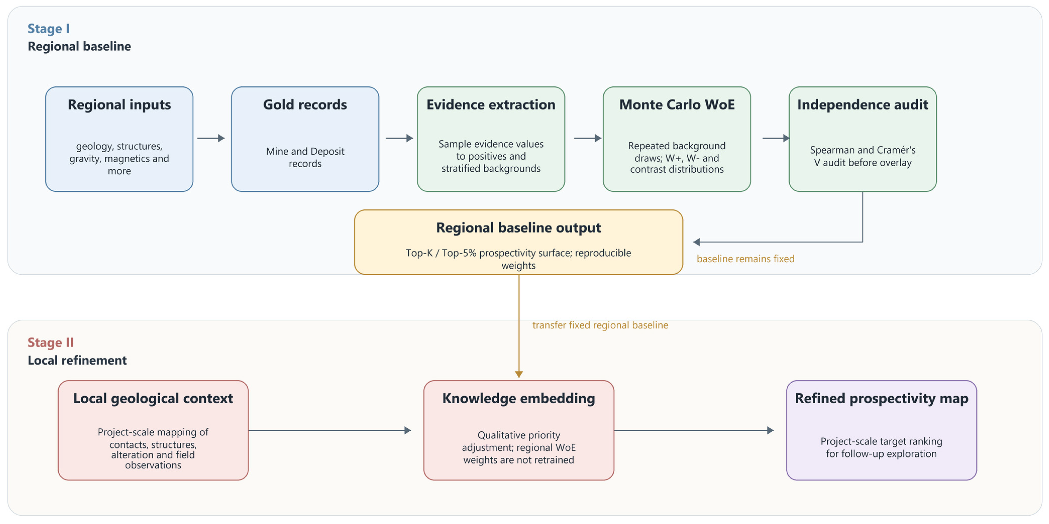
Here, we develop a robust sampled-WoE gold prospectivity workflow that links reproducible regional screening with separately reported project-scale geological interpretation. The regional baseline is trained across the Yilgarn Craton using stratified Monte Carlo sampling designed to reduce sensitivity to individual background samples. Evidence-layer dependence is explicitly audited before regional overlay. The reproducible regional Top-5% prospectivity zones can subsequently be transferred to project areas for local geological refinement without changing the regional sampled-WoE weights (
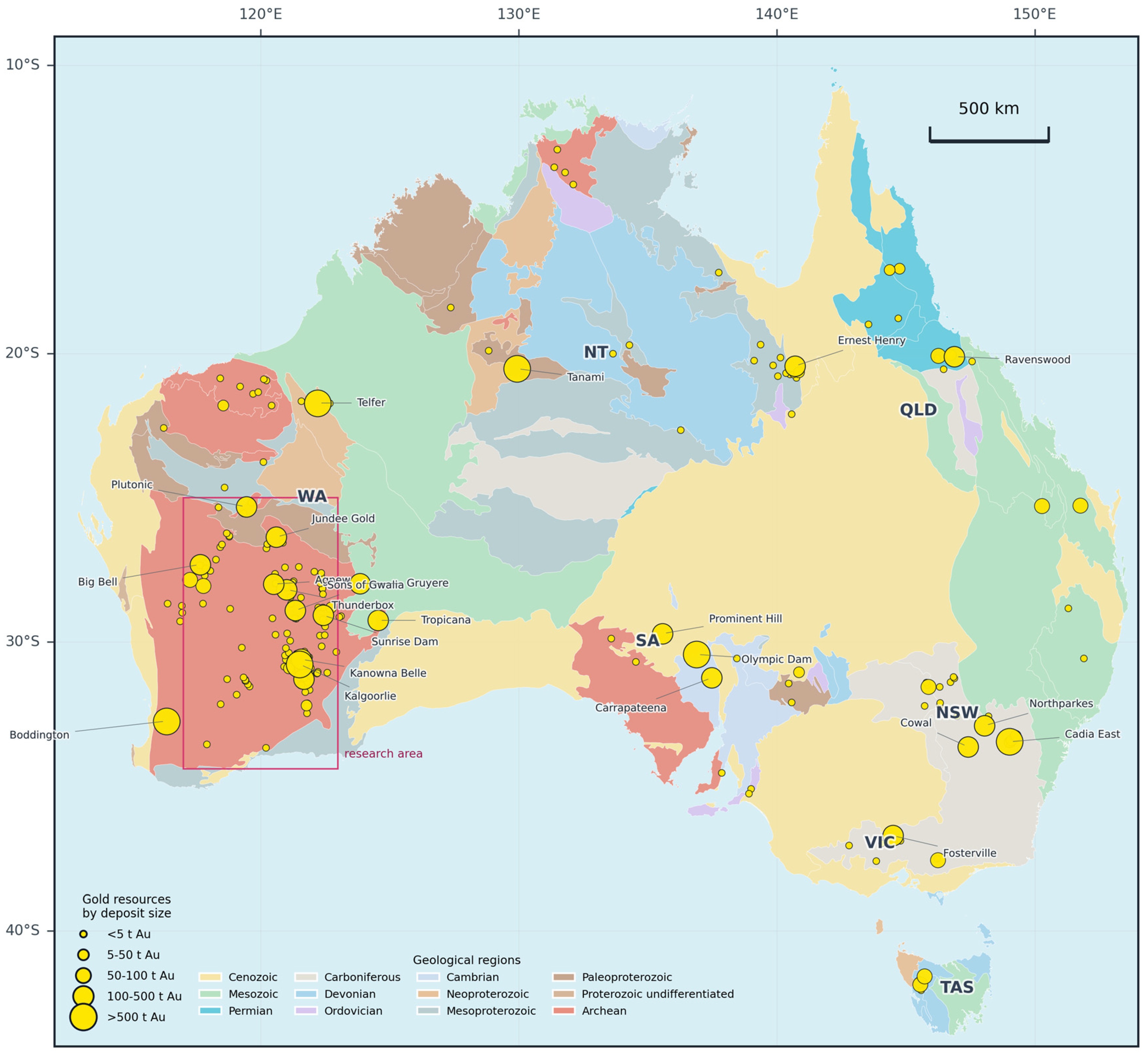
Figure 1).
This study makes four specific contributions beyond conventional WoE application. First, regional evidence weights are reported as distributions over repeated stratified background samples rather than as a single deterministic table, making background-selection sensitivity explicit. Second, negative weights are defined against sampled unlabeled background rather than assumed-barren ground, adapting the presence-background paradigm to mineral exploration. Third, an explicit Spearman and Cramér’s V independence audit is performed before overlay to respect the conditional-independence assumption of WoE. Fourth, a reproducible regional screening baseline is formally separated from interpretive project-scale refinement, removing the ambiguity between data-driven weighting and expert overlay. These contributions are method-general and are demonstrated here for orogenic gold in the Yilgarn Craton, where out-of-sample spatial cross-validation confirms that the workflow generalizes and outperforms naive single-layer and unit-weight baselines.
2. Geological Setting
2.1. The Yilgarn Craton
The Yilgarn Craton occupies > 600,000 km
2 of southwestern Australia and comprises three major tectonic components: the Youanmi Terrane, the Eastern Goldfields Superterrane, and the South West Terrane [
25,
26]. The Youanmi Terrane—subdivided into the Murchison and Southern Cross Domains—and the Eastern Goldfields Superterrane are characterized by granite-greenstone terranes with numerous greenstone belts interspersed with granites and gneisses [
25]. Deep seismic profiling reveals a complex crustal architecture with east-dipping reflectors beneath the Eastern Goldfields [
27], and recent isotopic studies have refined the craton’s internal stratigraphy [
28,
29] (
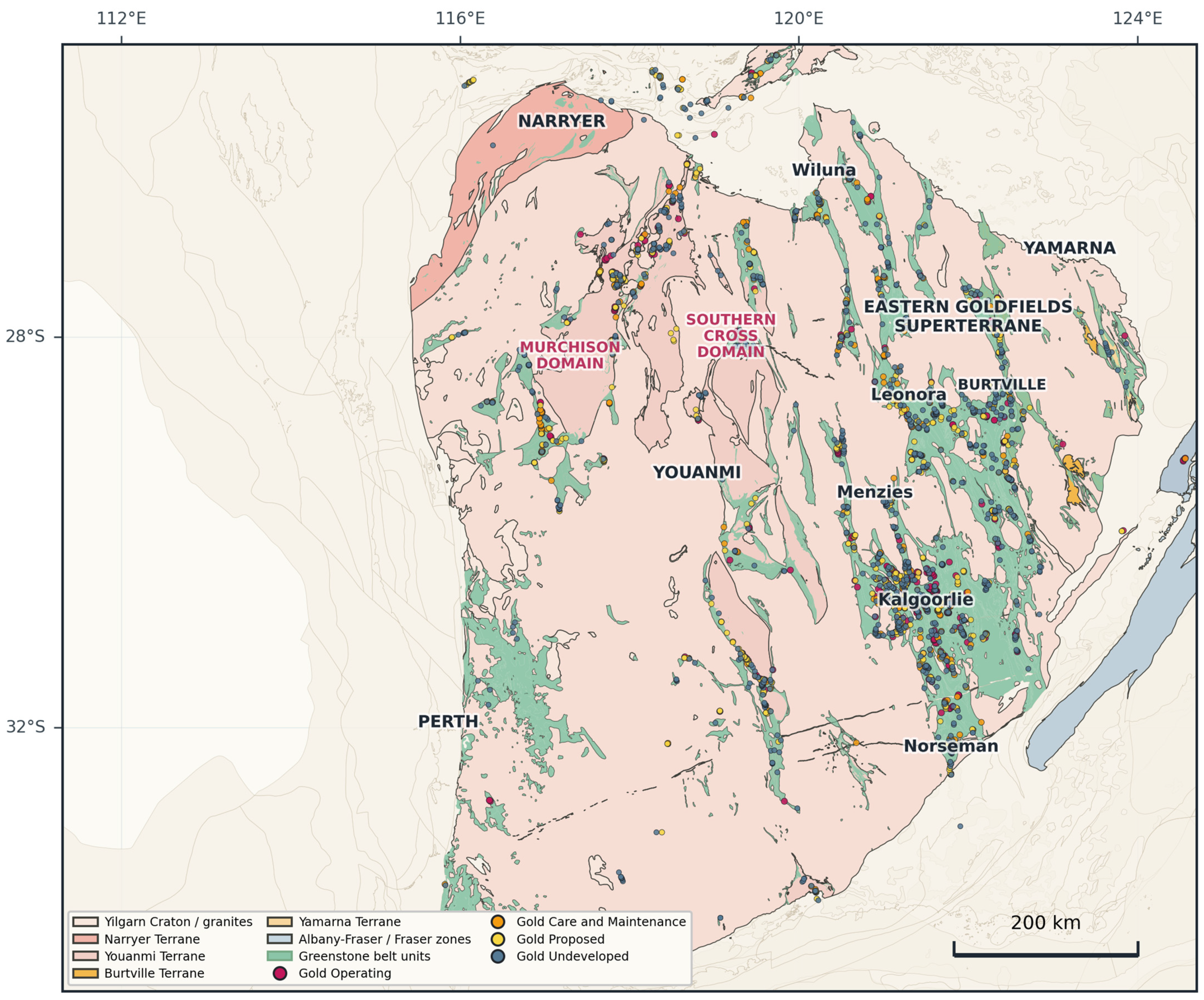
Figure 2).
2.2. Southern Cross Domain and the Marda-Diemals Greenstone Belt (MDGB)
The study area lies within the Southern Cross Domain, approximately 100 km south of the town of Southern Cross. Unlike adjacent terranes, the upper crust here largely lacks rocks amenable to precise geochronological dating [
30], though recent zircon U-Pb studies and regional 1:100,000 geological mapping provide key constraints on the local stratigraphic framework [
31,
32,
33,
34,
35,
36]. The MDGB provides the local project-scale geological context for the later knowledge-embedding stage; it is not the spatial extent of regional model training, which is conducted across the whole Yilgarn Craton.
Figure 2.
Geological subdivision map of the Yilgarn Craton, Western Australia (modified from [
29]).
Figure 2.
Geological subdivision map of the Yilgarn Craton, Western Australia (modified from [
29]).
The Clampton tenement package, located within the MDGB, has been explored intermittently since the 1960s. Early campaigns by Western Mining targeted base metals and nickel; subsequent work by Carpentaria Exploration, Roebuck Resources, Southern Cross Goldfields, and others progressively identified gold mineralization. Despite numerous exploration phases, no systematic data-driven prospectivity model has been developed for this region.
2.3. Orogenic Gold Mineralization
Gold deposits in the MDGB are classified as orogenic [
37,
38], a deposit type accounting for ~75% of global gold production [
39]. In the Yilgarn Craton, orogenic gold mineralization is spatially associated with major shear zones cutting greenstone belts, with multiple mineralization events spanning the Archean orogenic cycle [
40]. Within the Clampton area, gold is hosted by sheared mafic–ultramafic volcanic rocks along contact zones with metasedimentary units. Based on regional studies [
41], key exploration indicators include: (1) structural complexity at fault intersections and fold hinges; (2) favorable lithologies including tholeiitic basalt and BIF; (3) iron-rich host rocks in alteration zones; and (4) magnetic and gravity anomalies associated with fault-controlled fluid pathways and hydrothermal alteration systems [
42,
43].
3. Materials and Methods
3.1. Data Sources
Regional evidence layers were compiled for the Yilgarn Craton and clipped to a common study boundary (
Table 1). The formal training inputs comprise merged bedrock geology, an independent greenstone-belt footprint, merged structural linework, statewide magnetic and gravity grids, and airborne radiometric K, Th, U, and total-count grids. Structural linework was assembled using 1:100,000-scale data where available and 1:500,000-scale data to fill uncovered areas. Magnetic, gravity, and radiometric values were extracted to sample points at their native resolutions of 20 m, 400 m, and 80 m, respectively. Stream-sediment geochemistry was excluded because a spatially uniform Yilgarn-wide dataset was not available. Confidential project information was reserved for project-scale validation reported separately and was not used as a training evidence layer.
3.2. Statistical Analysis Framework
The regional sampled-WoE baseline was estimated from point samples. Strict Mine and Deposit gold records were spatially deduplicated using a 400 m grid so that densely recorded historical occurrences did not dominate the statistics; this cleaning step yielded 7203 representative mineralized points. Unlabeled background points were generated within the Yilgarn boundary and stratified by rock type, greenstone-belt membership, and fault-density class. Evidence values were extracted to mineralized and background points. Continuous evidence values were discretized using quintile breaks derived from the background candidate pool; duplicated break values caused by tied raster values were collapsed. Lithological setting was treated as a categorical variable. The 400 m grid was used for spatial deduplication and final map presentation, not for conventional cell-by-cell deposit counting.
3.3. GIS-Based Data Processing
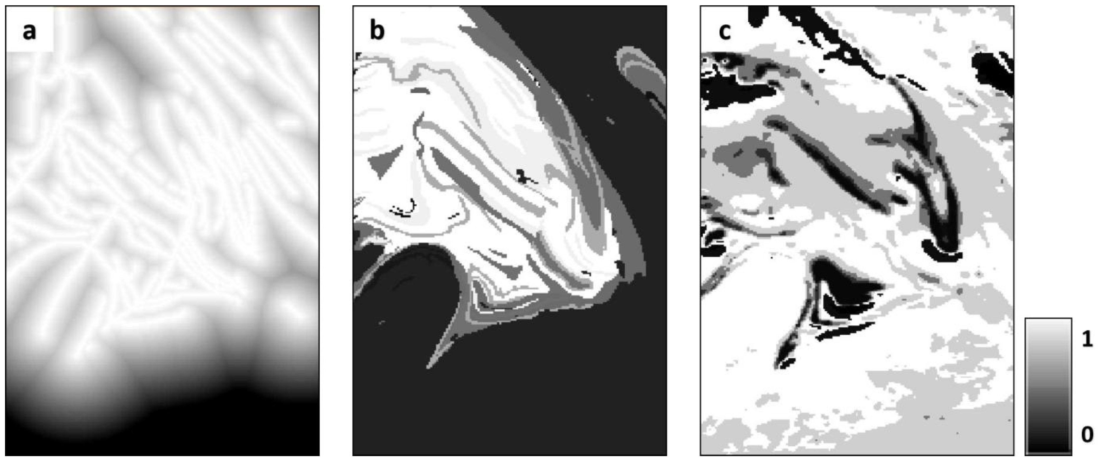
All formal regional layers were clipped to the Yilgarn boundary. Structural density was calculated using a 5 km moving-window radius. Distance to the nearest mapped fault or shear zone was calculated directly for sample points using a vector nearest-neighbor algorithm, while distance to structural intersections was retained as an alternative diagnostic layer. Geophysical values were extracted directly from their native source grids; no common-resolution resampling was required before point extraction. The regional output map was subsequently rendered on a 400 m presentation grid. The resulting secondary processing outputs are shown in
Figure 3.
3.4. Evidence-Layer Independence Audit
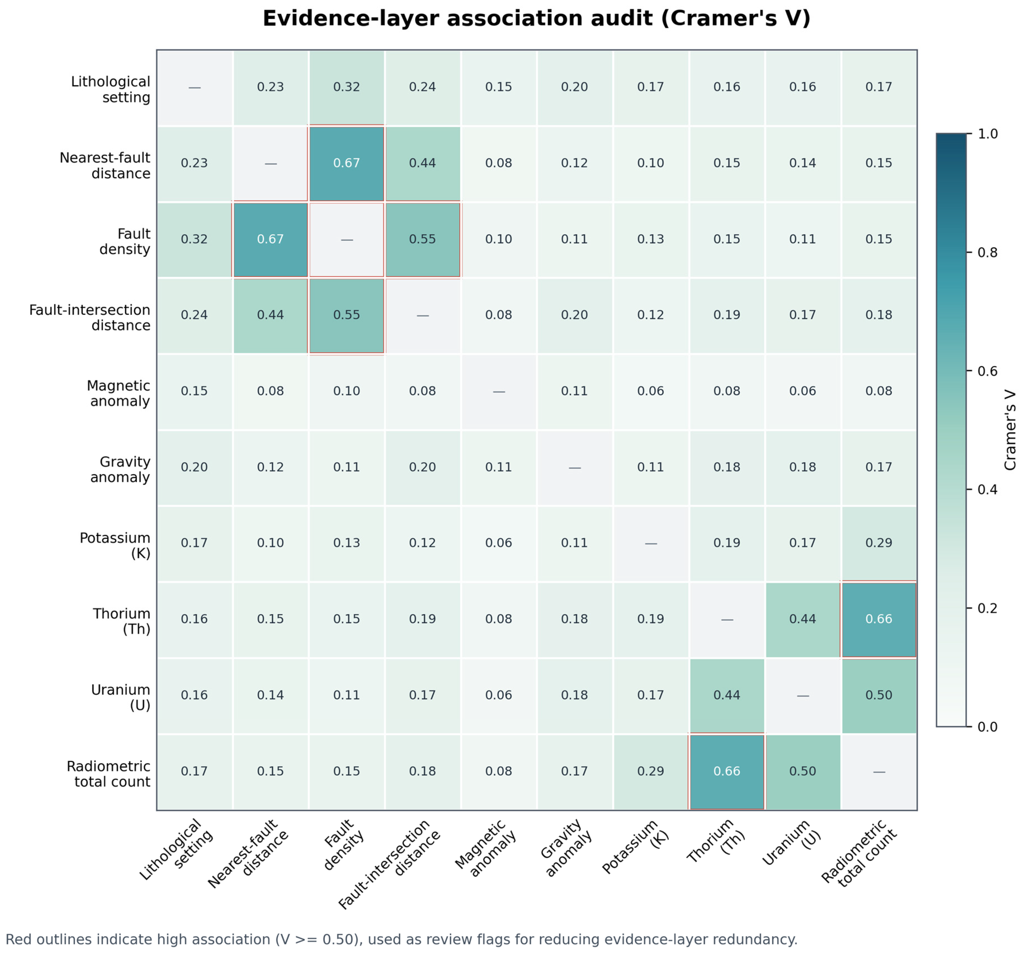
Ten evidence variables were initially retained for diagnostic assessment: lithological setting, fault density, distance to the nearest fault or shear zone, distance to structural intersections, magnetic anomaly, gravity anomaly, and K, Th, U, and total-count radiometrics. Dependence among continuous variables was evaluated using Spearman rank correlation, while binned evidence classes were assessed using Cramér’s V. Absolute Spearman rho values ≥ 0.70 and Cramér’s V values ≥ 0.50 were treated as high-dependence flags for review, rather than as automatic deletion rules.
Strong associations were identified between distance to the nearest structure and fault density (Spearman rho = −0.904; Cramér’s V = 0.673), between fault density and distance to structural intersections (Spearman rho = −0.718; Cramér’s V = 0.546), and among radiometric variables, particularly between Th and total count (Spearman rho = 0.950; Cramér’s V = 0.662). These relationships were treated as evidence-layer dependence rather than as additional predictive information.
To reduce double counting, one representative variable was retained from each strongly associated group after considering interpretability and geological role. Fault density was retained as the regional structural layer, while nearest-fault and intersection-distance variables were retained as diagnostics. Th was retained instead of total count and U, and K was retained as a complementary radiometric variable. The final regional overlay therefore comprised six layers: lithological setting, fault density, magnetic anomaly, gravity anomaly, K, and Th. The independence audit is summarized in
Figure 4.
3.5. Stratified Monte Carlo Sampled-WoE Baseline
For each Monte Carlo iteration, the representative mineralized points were held fixed and a new set of unlabeled background points was drawn using geological stratification. Background selection can influence presence–background models [
44]; repeated sampling was therefore used to report weight uncertainty rather than a single arbitrary background realization. For each evidence class E, positive and negative weights were calculated as:
where D denotes representative mineralized points and
denotes sampled unlabeled background points rather than confirmed barren locations;
denotes the complement of evidence class E.
The contrast C_E expresses the direction and strength of association. A Laplace smoothing constant of 0.5 was applied to stabilize low-frequency classes. The primary model used 14,406 background points per round, twice the number of representative mineralized points, with a 0 km exclusion buffer and 100 repeated sampling rounds. Stress testing evaluated eight scenarios and 800 rounds in total, including alternative random seeds, background-point ratios of 1×, 2×, and 5×, and exclusion buffers of 0, 2, 5, and 10 km. Final weights were estimated as the means across repeated background samples, accompanied by standard deviations, variances, and 95% intervals. For lithological combinations, support was defined as the summed number of representative mineralized samples and mean sampled-background records in a class. The support threshold of 30 was used as a conservative minimum count for estimating a stable log-ratio: below this level, a single occurrence or background draw can produce a disproportionate change in W_E
+ or W_E
−. Low-support lithological contrasts were therefore shrunk linearly toward zero by min(1, support/30) rather than discarded, preserving rare classes while preventing them from dominating the regional overlay. The mapping cap of [−3, 3] was applied only to lithological contrasts and corresponds to limiting any single lithological class to an odds-ratio contribution of approximately exp(3), so that one categorical layer cannot overwhelm the remaining five regional evidence layers. Representative favorable classes are summarized in
Table 2, and the overall regional-to-project workflow is shown in
Figure 5.
3.6. Project-Scale Geological Knowledge Refinement
The regional sampled-WoE baseline and project-scale geological interpretation were treated as separate stages. The reproducible regional model defines Top-5% prospectivity zones. Local geological knowledge can then be used to prioritize project-scale targets without altering the regional sampled-WoE weights. Project-scale verification is reported descriptively using confidential project data and is kept separate from the reproducible regional sampled-WoE baseline.
3.7. Spatial Cross-Validation
To assess out-of-sample performance and control for spatial autocorrelation, the regional baseline was evaluated with spatial-block cross-validation [
45]. The Yilgarn Craton was tiled into contiguous square blocks (primary size 100 km); whole blocks, rather than individual points, were assigned at random to five folds, and the assignment was repeated 20 times to average over partitioning choices. For each fold, the full sampled-WoE estimation (evidence binning, positive and negative weights, contrast, Laplace smoothing of 0.5, and the sparse-lithology regularization) was repeated using only the training folds, and the resulting weights were applied to the held-out fold, where the Top-5% capture was measured against the held-out area. A non-spatial random five-fold cross-validation was run for comparison, and block sizes of 50, 100, and 150 km were tested for sensitivity.
4. Results
4.1. Fault–Mineralization Relationships
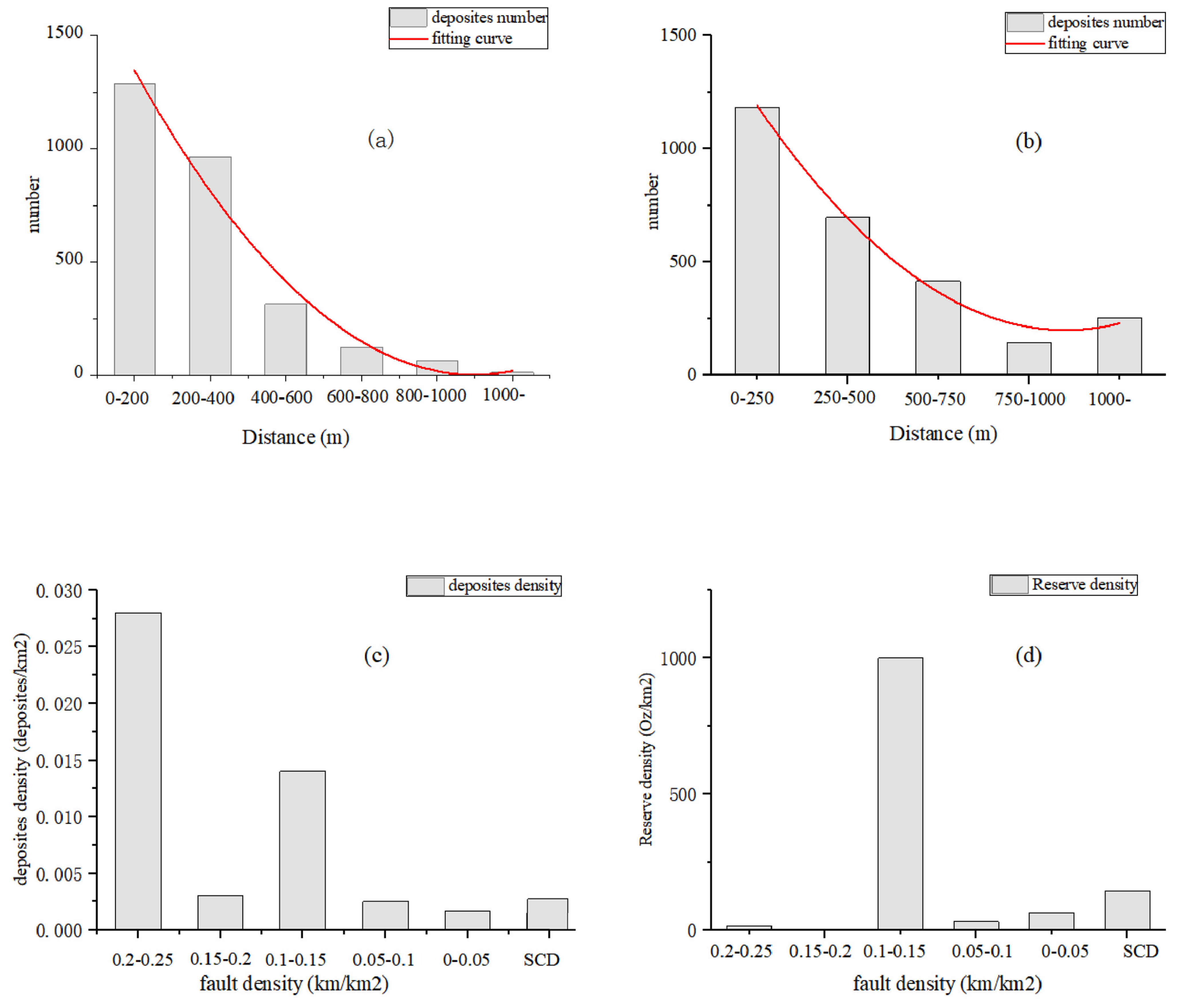
Point-based diagnostic analysis indicates that mapped faults and shear zones remain important regional controls on gold distribution. Fault-related variables were evaluated through nearest-structure distance, distance to structural intersections, and fault density. Because these variables partly encode the same structural information, fault density was retained as the representative structural layer in the final six-layer stack. The high-density interval (>0.261) produced a favorable contrast of 2.169, whereas the low-density interval (≤0.113) produced a negative contrast of −2.297.
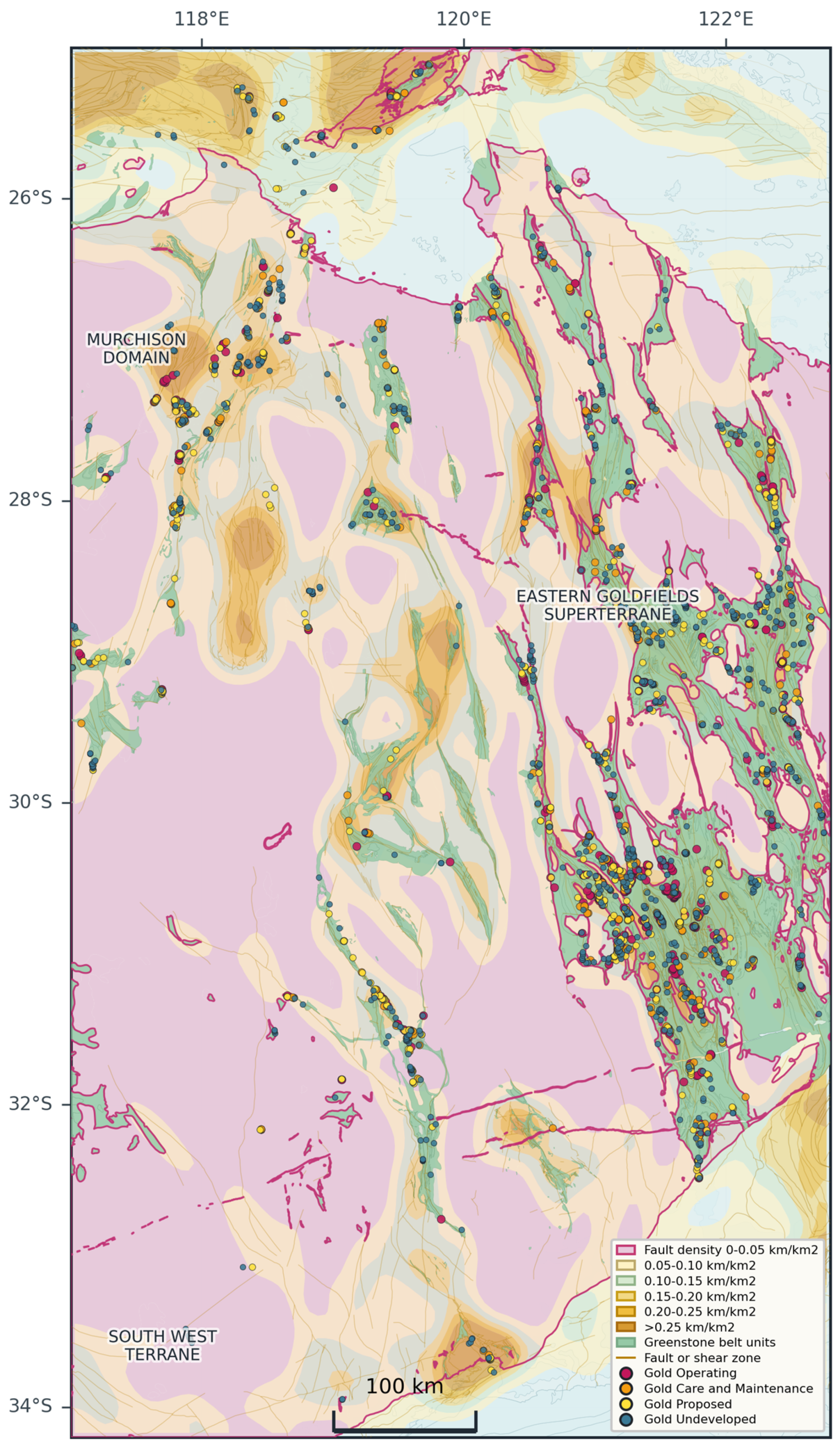
The use of a representative structural layer avoids repeatedly counting the same geological control while retaining the broad structural corridors required for regional screening. Nearest-structure distance and intersection distance remain available as diagnostic alternatives. The spatial pattern of fault density and gold records is shown in
Figure 6, and the structural-variable relationships are shown in
Figure 7.
4.2. Lithological Controls
Lithological setting was represented by the combination of merged bedrock rock type and independent greenstone-belt membership. This formulation captures regional lithological associations without relying on a manually assigned expert score. Fifty-four lithological combinations were evaluated. Thirty-one classes had adequate support, whereas 23 low-support combinations with total support below 30 were conservatively regularized before final mapping using C_regularized = C_raw × min(1, support/30), and lithological contrasts were capped to the range [−3, 3]. In the audit table, four raw lithological contrasts exceeded an absolute value of 3 before capping; after shrinkage and capping no lithological mapping contrast exceeded this range. The strongest sparse-class raw contrast was reduced from 3.163 to 1.897, illustrating that the procedure dampens rare categories rather than creating favorable lithological weights. The complete auditable lithological table is reported in
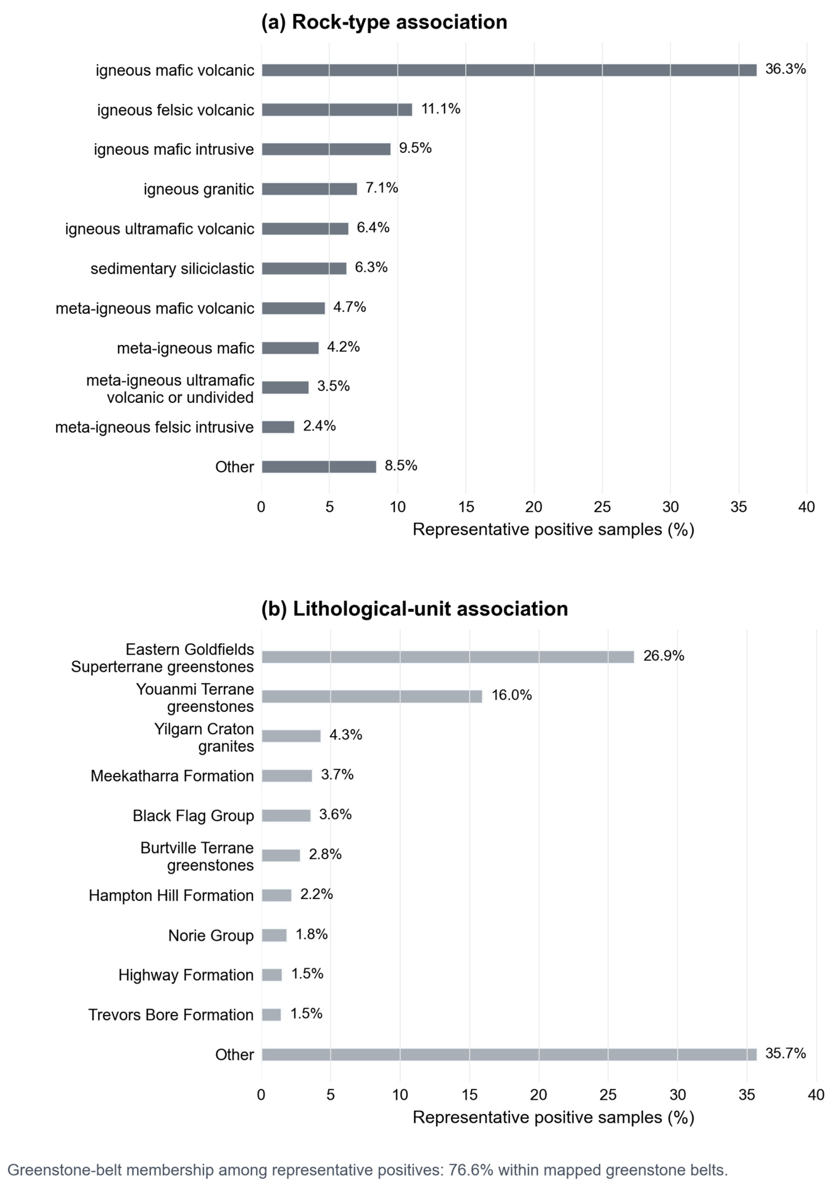
Supplementary Materials. Representative lithological associations are shown in
Figure 8.
4.3. Geophysical Signatures
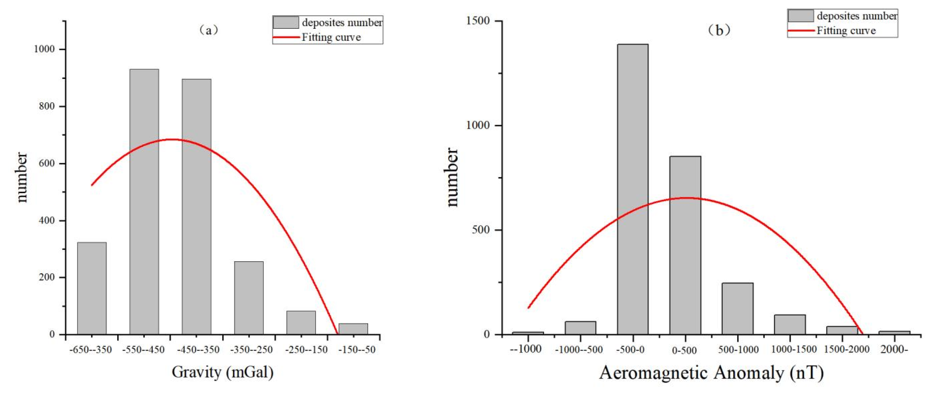
Magnetic and gravity grids were sampled directly at mineralized and background points. Both variables were retained because they provide complementary information on crustal architecture, lithological contrasts, and structural corridors. Representative favorable contrasts were 0.761 for magnetic anomalies ≤ −129.312 and 1.010 for gravity anomalies from −510.668 to −365.907. The geophysical relationships are shown in
Figure 9.
Figure 6.
Regional distribution of fault density, greenstone-belt outlines, and gold records across the Yilgarn Craton.
Figure 6.
Regional distribution of fault density, greenstone-belt outlines, and gold records across the Yilgarn Craton.
Figure 7.
Relationship between gold deposits and structural variables: (a) distance to faults; (b) distance to fault intersections; (c) fault density; and (d) fault-related host-rock reserve density.
Figure 7.
Relationship between gold deposits and structural variables: (a) distance to faults; (b) distance to fault intersections; (c) fault density; and (d) fault-related host-rock reserve density.
4.4. Radiometric Signatures
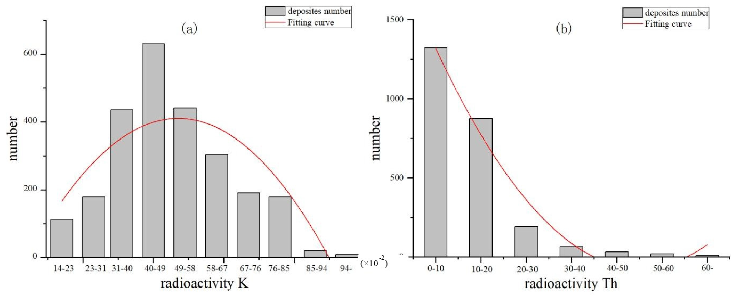
K, Th, U, and total-count radiometric variables were evaluated diagnostically. The independence audit showed a strong association among several radiometric layers, particularly between Th and total count. K and Th were therefore retained as representative radiometric variables, while U and total count were reserved as diagnostic alternatives. Representative favorable contrasts were 1.063 for K values from 0.46 to 0.72 and 1.287 for Th values ≤ 7.854. In contrast, Th values > 24.865 produced a negative contrast of −2.935. The radiometric relationships are shown in
Figure 10.
Figure 8.
Lithological association of representative positive gold samples: (a) rock-type distribution (b) lithological-unit distribution.
Figure 8.
Lithological association of representative positive gold samples: (a) rock-type distribution (b) lithological-unit distribution.
Figure 9.
Relationship between gold deposits and geophysical anomalies: (a) gravity anomaly and (b) aeromagnetic anomaly.
Figure 9.
Relationship between gold deposits and geophysical anomalies: (a) gravity anomaly and (b) aeromagnetic anomaly.
Figure 10.
Relationship between gold deposits and airborne radiometric anomalies: (a) potassium (K) and (b) thorium (Th).
Figure 10.
Relationship between gold deposits and airborne radiometric anomalies: (a) potassium (K) and (b) thorium (Th).
4.5. Prospectivity Mapping
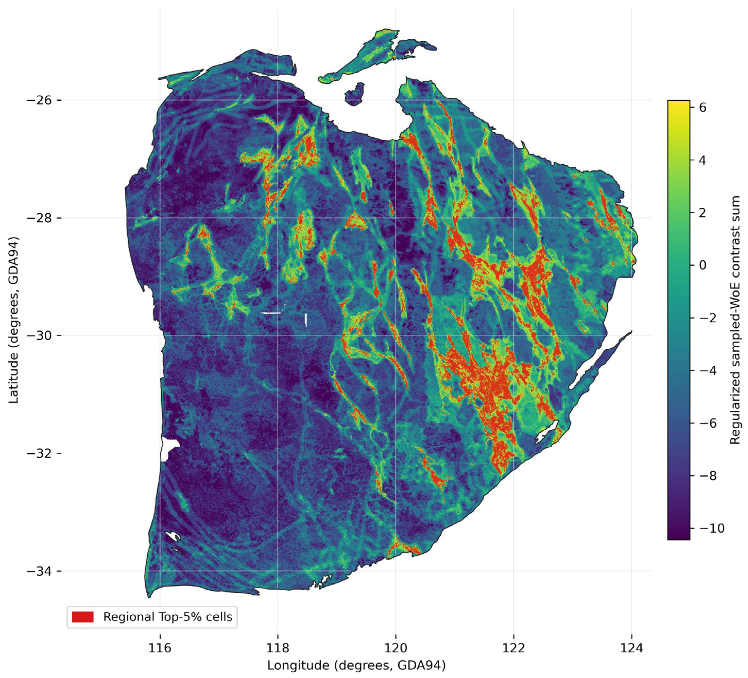
Across alternative random seeds, representative favorable contrasts varied by no more than 0.00584; changing the background-point ratio from 1× to 5× produced variations of no more than 0.00567. By contrast, increasing the exclusion buffer from 0 to 10 km inflated representative favorable contrasts by 2.4% to 38.5%, with the largest increases for magnetic anomalies (+38.5%), K (+26.1%), and fault density (+24.9%). The conservative 0 km scenario was therefore selected for regional mapping. The six-layer baseline was rendered across the Yilgarn Craton on a 400 m output grid containing 3,814,732 valid cells. Cells were ranked by their regularized sampled-WoE contrast sum and the highest-ranked 5% were classified as regional high-potential zones. A separate sparse-lithology audit further confirmed that the regularization mainly affected rare categories: 23 of 54 lithological combinations were flagged for review, all were retained with reduced influence, and the cap affected only four raw lithological contrasts. Because the final Top-5% map is produced from a six-layer evidence stack, this treatment constrains empirical outliers in the categorical lithology layer while leaving adequately supported lithologies unchanged. The regional prospectivity map is shown in
Figure 11.
4.6. Regional Screening Performance and Project-Scale Validation
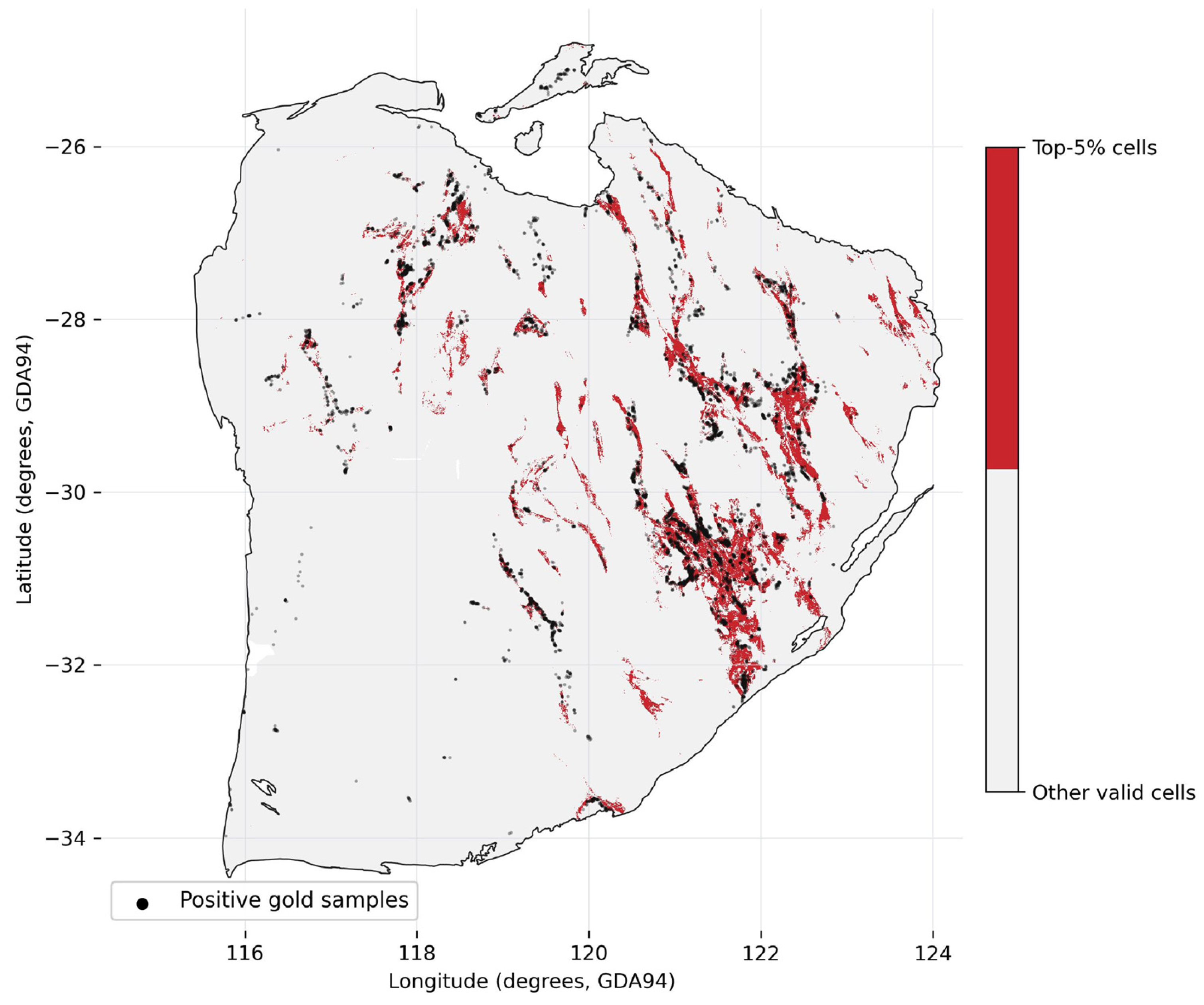
Regional model behavior was summarized using a Top-K area-capture metric. The highest-ranked 5% of the valid Yilgarn output area captured 3544 of 7199 valid representative mineralized points, corresponding to a descriptive training-sample capture rate of 49.23% and a 9.85-fold enrichment over random spatial selection. Four of the 7203 representative mineralized points were excluded from this calculation because at least one formal regional evidence value was missing. This value quantifies regional enrichment and is not presented as independent-validation recall. Separately, spatial-block cross-validation was used as the out-of-sample test for spatial prediction, following common recommendations for spatially structured data and prediction-rate validation [
45,
46]. The primary 100 km, five-fold spatial-block test retained a 45.4% Top-5% capture and 9.1-fold enrichment, distinguishing the reproducible training-sample Top-K result from out-of-sample model performance. The Top-5% zones and regional screening summary are shown in
Figure 12 and
Table 3.
Figure 11.
Yilgarn regional sampled-WoE baseline and Top-5% prospectivity zones.
Figure 11.
Yilgarn regional sampled-WoE baseline and Top-5% prospectivity zones.
Figure 12.
Yilgarn regional sampled-WoE Top-5% prospectivity zones with representative positive gold samples.
Figure 12.
Yilgarn regional sampled-WoE Top-5% prospectivity zones with representative positive gold samples.
Project-scale verification was performed in the Clampton tenement package within the Marda-Diemals Greenstone Belt by applying the regional sampled-WoE weights to the local evidence layers and refining the overlay with project-scale geological knowledge. This step did not modify the regional weights; instead, it transferred the reproducible regional baseline to the project area and incorporated locally mapped structures, host-rock contacts, and alteration controls reported in the internal exploration record.
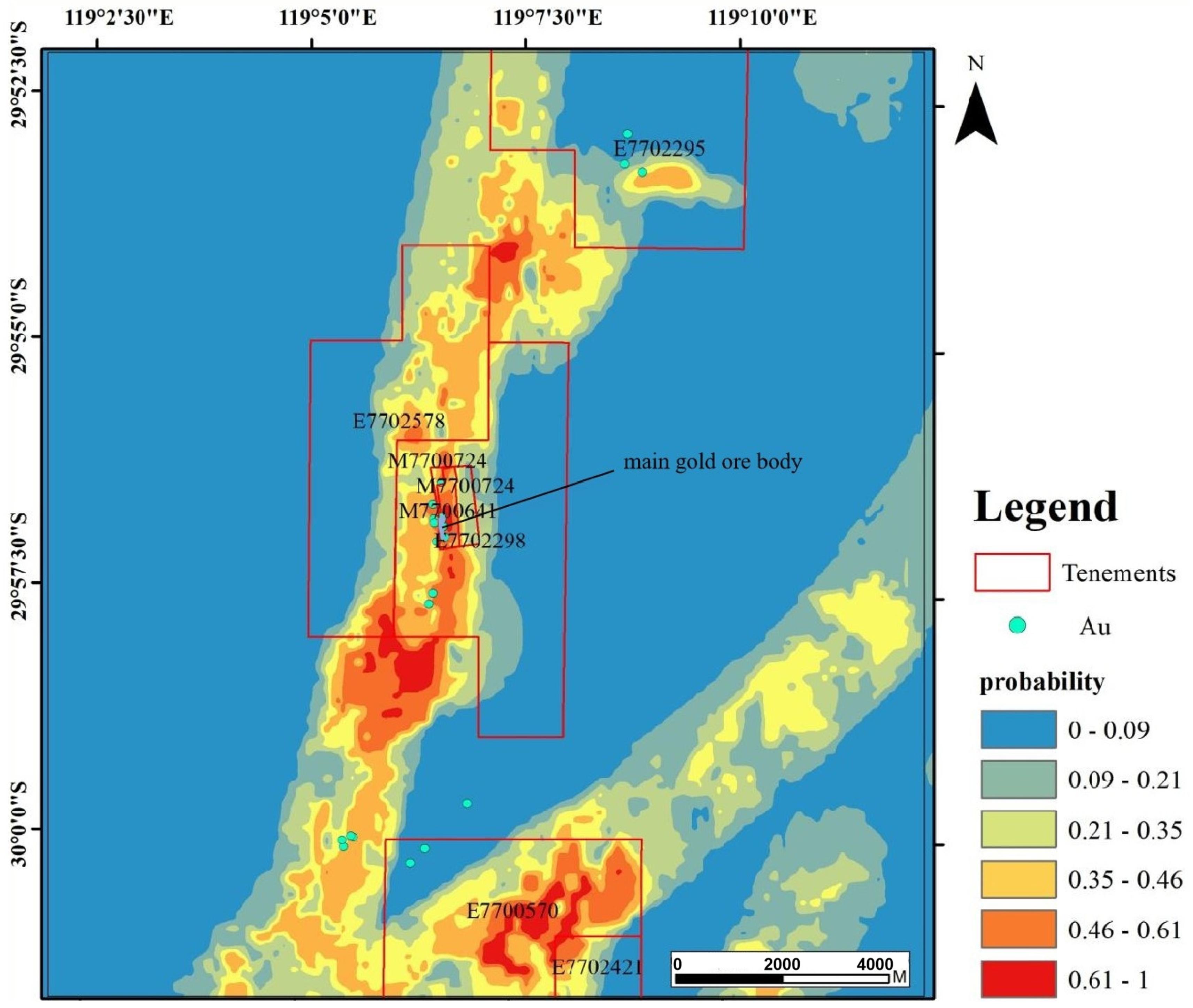
The project-scale prediction map (
Figure 13) delineates coherent high-potential corridors that follow contacts between mafic volcanic host rocks and metasedimentary sequences and that intersect mapped structural complexities, in agreement with the regional structural and lithological associations identified in
Section 4. The Andromeda prospect is recovered without any project-specific re-weighting, and additional clusters of favorable cells highlight previously underexplored corridors at greenstone-belt margins.
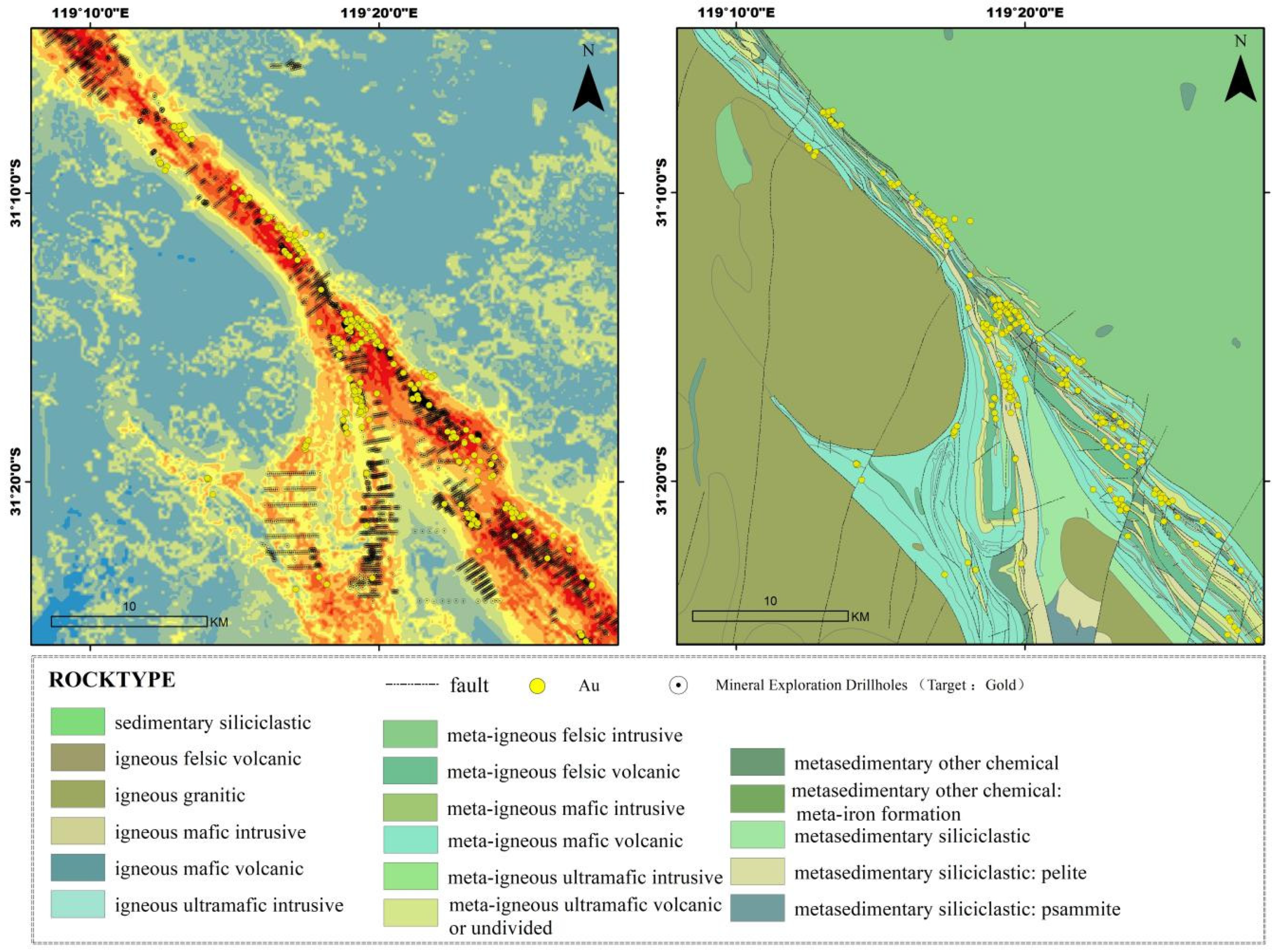
Partial verification against the available mineralized-sample distribution (
Figure 14) shows that known gold occurrences fall predominantly within the project-scale high-potential zones produced by the locally refined overlay. This verification is reported as a descriptive coincidence between the locally refined map and the available samples within the confidential project dataset, and is not presented as an independent statistical validation of the regional weights.
4.7. Out-of-Sample Spatial Cross-Validation
To provide an out-of-sample assessment and to control for spatial autocorrelation, the regional baseline was evaluated with spatial-block cross-validation (
Section 3.7). A from-scratch re-estimation reproduced the released weights (for example, fault-density contrasts of −2.298, −0.101, and +2.167 against published values of −2.297, −0.104, and +2.169) and an in-sample Top-5% capture of 49.6%, consistent with the descriptive 49.23% reported in
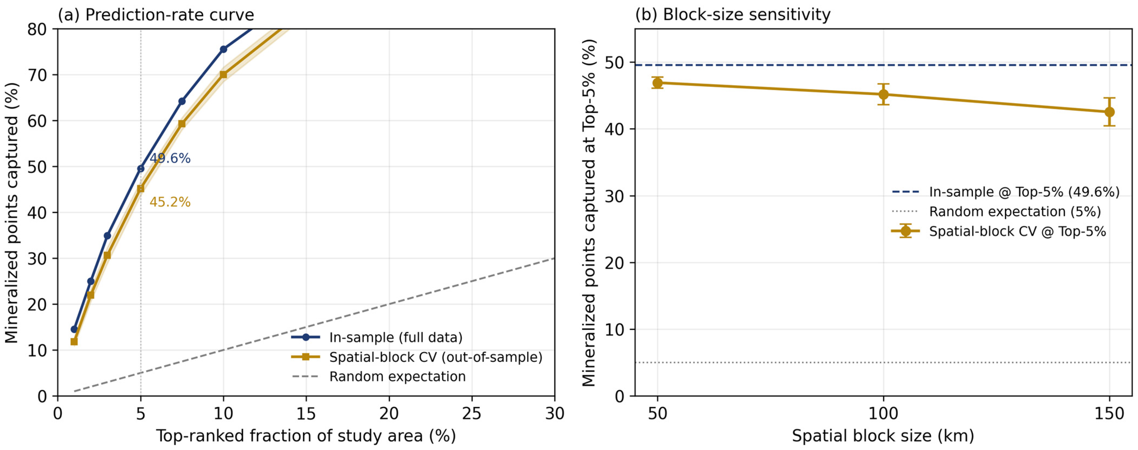
Section 4.6. Under spatial-block cross-validation (100 km blocks, five folds, 20 random block-to-fold assignments), the out-of-sample Top-5% capture was 45.4% (standard deviation 1.5%), a 9.1-fold enrichment over random selection (
Table 4). A non-spatial random five-fold cross-validation returned 49.3%, statistically indistinguishable from the in-sample value, confirming that random cross-validation is optimistically biased by spatial autocorrelation and that spatial blocking removes approximately four percentage points of this optimism. The result was stable across block sizes (46.8%, 45.4%, and 42.1% capture at 50, 100, and 150 km;
Figure 15b), and the prediction-rate curve exceeded the random expectation at all cut-offs (
Figure 15a). To confirm that the multi-layer model adds value over trivial alternatives, the full six-layer model was benchmarked under the same cross-validation against a single fault-density layer and a unit-weight overlay; on an area-matched basis the full model was superior at every cut-off (
Table 5), resolving the top 1% of the area at 11.7-fold enrichment, whereas a single structural layer could nominate only a coarse 20% of the area at 3.4-fold enrichment. The validation curves and block-size sensitivity analysis are shown in
Figure 15.
5. Discussion
The framework separates a reproducible regional sampled-WoE baseline from project-scale geological interpretation. This distinction avoids ambiguity between conditional-probability WoE and expert weighted overlay.
First, repeated geological-stratified sampling addresses sensitivity to any single set of unlabeled background points. The regional weights are reported as distributions rather than as a single deterministic table. Representative favorable contrasts varied by ≤0.00584 across alternative random seeds and by ≤0.00567 as the background-point ratio increased from 1× to 5×. Larger exclusion buffers were more consequential because they systematically removed favorable near-deposit background samples. The sparse-lithology rule should therefore be interpreted as a conservative stability control rather than as an additional geological assumption: adequate lithological classes retain their sampled-WoE contrasts, while low-support classes are kept in the map but assigned reduced leverage.
Second, the evidence-layer independence audit addresses a central assumption of WoE overlay. Spearman correlation and Cramér’s V identified groups of related variables using review flags of |rho| ≥ 0.70 and V ≥ 0.50. Restricting the final overlay to six representative layers reduces double counting while preserving diagnostic alternatives.
Third, the regional Top-5% zones are intended as a reproducible screening output rather than a substitute for local geological interpretation. At project scale, geological knowledge can refine target priorities without being presented as a recalculated regional WoE probability surface.
Several limitations remain. A spatially uniform Yilgarn-wide stream-sediment geochemical dataset was not available and geochemistry was therefore excluded from the formal regional stack. Some lithological combinations have limited sample support and were conservatively regularized before mapping; the support threshold and contrast cap are empirical stability controls, and the complete regularization audit is therefore supplied so that future users can test alternative thresholds if larger training datasets become available. Larger gold-point exclusion buffers systematically inflated several evidence contrasts; the no-buffer scenario was therefore selected as the conservative primary model. Finally, project-scale refinement remains interpretive and should be evaluated separately using confidential project-scale validation data.
The independence audit controls pairwise dependence among evidence layers but does not guarantee full conditional independence given mineralization; the spatial-block cross-validation in
Section 4.7 therefore provides an out-of-sample check on the combined model, and the 45.4% out-of-sample capture (versus 49.3% under random folds) shows that the workflow generalizes while quantifying the spatial-autocorrelation optimism that would otherwise inflate apparent performance.
Building on the spatial-block cross-validation reported in
Section 4.7, future work should extend the withheld-area evaluation to additional terranes and commodity types, evaluate alternative discretization strategies, and examine how local geological interpretation modifies project-scale target ranking without changing the reproducible regional baseline.
6. Conclusions
This study presents a robust sampled-WoE gold prospectivity workflow for the Yilgarn Craton. The key findings are:
- (1)
A point-based regional baseline was constructed from 7203 spatially deduplicated representative mineralized points and repeatedly sampled unlabeled background points.
- (2)
An evidence-layer independence audit reduced ten diagnostic variables to a six-layer regional stack: lithological setting, fault density, magnetic anomaly, gravity anomaly, K, and Th.
- (3)
Stratified Monte Carlo sampled-WoE produced stable regional evidence weights. The highest-ranked 5% of the study area captured 49.23% of valid representative mineralized points, a descriptive 9.85-fold enrichment over random spatial selection.
- (4)
The reproducible regional Top-5% zones provide a consistent basis for subsequent project-scale geological refinement and separately reported descriptive project-scale verification.
The workflow provides a transparent regional screening baseline while preserving the distinct role of geological interpretation in project-scale exploration decisions.
Author Contributions
Conceptualization, Y.L.; methodology, Y.L.; software, Y.L.; validation, Y.L. and Y.S.; formal analysis, Y.L.; investigation, Y.L., Y.S. and J.T.; resources, X.W.; data curation, Y.L. and J.T.; writing—original draft preparation, Y.L.; writing—review and editing, X.W., X.Z., Y.S. and J.T.; visualization, Y.L. and Y.S.; supervision, X.W.; project administration, X.W.; and funding acquisition, X.W. All authors have read and agreed to the published version of the manuscript.
Funding
This research was supported by internal industry funding from GeoVision AI and Delta Resource Group. No grant number was assigned.
Data Availability Statement
Public geological and geophysical datasets supporting this study are available from the Geological Survey of Western Australia and Geoscience Australia. Proprietary project-scale drilling and exploration datasets are not publicly available due to confidentiality restrictions.
Acknowledgments
We are grateful to AUKT for generously providing original exploration data and logistical support during visits to the study area.
Conflicts of Interest
Yang Luo is employed by the company GeoVision AI., Xinyu Zou, Xuance Wang, Yue Song and Jiaxu Tang are employed by the company LynAI Mines Ltd. The authors declare no conflicts of interest. The funders had no role in the design of the regional sampled-WoE workflow, public-data analysis, or manuscript preparation. Proprietary project data were used only for descriptive project-scale verification.
References
- Schodde, R. Long Term Trends in Global Exploration—Are We Finding Enough Metal. In Proceedings of the 11th Fennoscandian Exploration and Mining Conference, Levi, Finland, 31 October 2017; p. 31. [Google Scholar]
- Bonham-Carter, G.F. Geographic Information Systems for Geoscientists: Modelling with GIS; Elsevier: Amsterdam, The Netherlands, 1994; Volume 13. [Google Scholar]
- Harris, D.V.P. Mineral Resources Appraisal: Mineral Endowment, Resources, and Potential Supply: Concepts, Methods and Cases; Clarendon Press: Oxford, UK, 1984. [Google Scholar]
- Agterberg, F.P. Automatic Contouring of Geological Maps to Detect Target Areas for Mineral Exploration. J. Int. Assoc. Math. Geol. 1974, 6, 373–395. [Google Scholar] [CrossRef] [Scilit]
- Carranza, E.J.M. Geochemical Anomaly and Mineral Prospectivity Mapping in GIS; Elsevier: Amsterdam, The Netherlands, 2008. [Google Scholar]
- Porwal, A.; Carranza, E.J.M.; Hale, M. Knowledge-Driven and Data-Driven Fuzzy Models for Predictive Mineral Potential Mapping. Nat. Resour. Res. 2003, 12, 1–25. [Google Scholar] [CrossRef] [Scilit]
- McKay, G.; Harris, J.R. Comparison of the Data-Driven Random Forests Model and a Knowledge-Driven Method for Mineral Prospectivity Mapping: A Case Study for Gold Deposits around the Huritz Group and Nueltin Suite, Nunavut, Canada. Nat. Resour. Res. 2016, 25, 125–143. [Google Scholar] [CrossRef] [Scilit]
- Porwal, A.; Carranza, E.J.M.; Hale, M. A Hybrid Fuzzy Weights-of-Evidence Model for Mineral Potential Mapping. Nat. Resour. Res. 2006, 15, 1–14. [Google Scholar] [CrossRef] [Scilit]
- Skirrow, R.G.; Campbell, I.H.; Zaw, K. Mapping Iron Oxide Cu-Au (IOCG) Mineral Potential in Australia Using a Knowledge-Driven Mineral Systems-Based Approach. Ore Geol. Rev. 2019, 113, 103011. [Google Scholar] [CrossRef] [Scilit]
- Boadi, B.; Raju, P.S.; Wemegah, D.D. Analysing Multi-Index Overlay and Fuzzy Logic Models for Lode-Gold Prospectivity Mapping in the Ahafo Gold District—Southwestern Ghana. Ore Geol. Rev. 2022, 148, 105059. [Google Scholar] [CrossRef] [Scilit]
- Harris, J.R.; Grunsky, E.; Behnia, P.; Corrigan, D. Data- and Knowledge-Driven Mineral Prospectivity Maps for Canada’s North. Ore Geol. Rev. 2015, 71, 788–803. [Google Scholar] [CrossRef] [Scilit]
- Kreuzer, O.P.; Yousefi, M.; Nykänen, V. Introduction to the Special Issue on Spatial Modelling and Analysis of Ore-Forming Processes in Mineral Exploration Targeting. Ore Geol. Rev. 2020, 119, 103391. [Google Scholar] [CrossRef] [Scilit]
- Carranza, E.J.M.; Van Ruitenbeek, F.J.A.; Hecker, C.; van der Meijde, M.; van der Meer, F.D. Knowledge-Guided Data-Driven Evidential Belief Modeling of Mineral Prospectivity in Cabo de Gata, SE Spain. Int. J. Appl. Earth Obs. Geoinf. 2008, 10, 374–387. [Google Scholar] [CrossRef] [Scilit]
- Rodriguez-Galiano, V.; Sanchez-Castillo, M.; Chica-Olmo, M.; Chica-Rivas, M.J. Machine Learning Predictive Models for Mineral Prospectivity: An Evaluation of Neural Networks, Random Forest, Regression Trees and Support Vector Machines. Ore Geol. Rev. 2015, 71, 804–818. [Google Scholar] [CrossRef] [Scilit]
- Koike, K.; Matsuda, S.; Suzuki, T.; Ohmi, M. Neural Network-Based Estimation of Principal Metal Contents in the Hokuroku District, Northern Japan, for Exploring Kuroko-Type Deposits. Nat. Resour. Res. 2002, 11, 135–156. [Google Scholar] [CrossRef] [Scilit]
- Porwal, A.; Gonzalez-Alvarez, I.; Markwitz, V.; McCuaig, T.C.; Mamuse, A. Weights-of-Evidence and Logistic Regression Modeling of Magmatic Nickel Sulfide Prospectivity in the Yilgarn Craton, Western Australia. Ore Geol. Rev. 2010, 38, 184–196. [Google Scholar] [CrossRef] [Scilit]
- Sun, T.; Xie, Z.; Liu, J. Data-Driven Predictive Modelling of Mineral Prospectivity Using Machine Learning and Deep Learning Methods: A Case Study from Southern Jiangxi Province, China. Minerals 2020, 10, 102. [Google Scholar] [CrossRef] [Scilit]
- Ding, K.; Xue, L.; Ran, X.; Wang, J.; Yan, Q. Siamese Network Based Prospecting Prediction Method: A Case Study from the Au Deposit in the Chongli Mineral Concentrate Area in Zhangjiakou, Hebei Province, China. Ore Geol. Rev. 2022, 148, 105024. [Google Scholar] [CrossRef] [Scilit]
- Ghezelbash, R.; Maghsoudi, A.; Bigdeli, A.; Carranza, E.J.M. Regional-Scale Mineral Prospectivity Mapping: Support Vector Machines and an Improved Data-Driven Multi-Criteria Decision-Making Technique. Nat. Resour. Res. 2021, 30, 1977–2005. [Google Scholar] [CrossRef] [Scilit]
- Blewett, R.S.; Czarnota, K.; Henson, P.A. Structural-Event Framework for the Eastern Yilgarn Craton, Western Australia, and Its Implications for Orogenic Gold. Precambrian Res. 2010, 183, 203–229. [Google Scholar] [CrossRef] [Scilit]
- Blenkinsop, T.G.; Doyle, M.G. Structural Controls on Gold Mineralization on the Margin of the Yilgarn Craton, Albany–Fraser Orogen: The Tropicana Deposit, Western Australia. J. Struct. Geol. 2014, 67, 189–204. [Google Scholar] [CrossRef] [Scilit]
- Witt, W.K.; Ford, A.; Hanrahan, B.; Mamuse, A. Regional-Scale Targeting for Gold in the Yilgarn Craton: Part 1 of the Yilgarn Gold Exploration Targeting Atlas; Geological Survey of Western Australia: Perth, Australia, 2013.
- Witt, W.K.; Ford, A.; Hanrahan, B. District-Scale Targeting for Gold in the Yilgarn Craton: Part 2 of the Yilgarn Gold Exploration Targeting Atlas; Geological Survey of Western Australia: Perth, Australia, 2015; Volume 132.
- Senior, A. Australian Resource Reviews: Gold 2019; Geoscience Australia: Canberra, Australia, 2019.
- Anand, R.R.; Paine, M. Regolith Geology of the Yilgarn Craton, Western Australia: Implications for Exploration. Aust. J. Earth Sci. 2002, 49, 3–162. [Google Scholar] [CrossRef] [Scilit]
- Cassidy, K.F.; Champion, D.C.; Krapez, B.; Barley, M.E.; Brown, S.J.A.; Blewett, R.S.; Tyler, I.M. A Revised Geological Framework for the Yilgarn Craton, Western Australia. Geol. Surv. West. Aust. Rec. 2006, 8, 15. [Google Scholar]
- Drummond, B.J.; Goleby, B.R.; Swager, C.P. Crustal Signature of Late Archaean Tectonic Episodes in the Yilgarn Craton, Western Australia: Evidence from Deep Seismic Sounding. Tectonophysics 2000, 329, 193–221. [Google Scholar] [CrossRef] [Scilit]
- Pawley, M.J.; Wingate, M.T.D.; Kirkland, C.L.; Wyche, S.; Hall, C.E.; Romano, S.S.; Doublier, M.P. Adding Pieces to the Puzzle: Episodic Crustal Growth and a New Terrane in the Northeast Yilgarn Craton, Western Australia. Aust. J. Earth Sci. 2012, 59, 603–623. [Google Scholar] [CrossRef] [Scilit]
- Wyche, S.; Kirkland, C.L.; Riganti, A.; Pawley, M.J.; Belousova, E.; Wingate, M.T.D. Isotopic Constraints on Stratigraphy in the Central and Eastern Yilgarn Craton, Western Australia. Aust. J. Earth Sci. 2012, 59, 657–670. [Google Scholar] [CrossRef] [Scilit]
- Bloem, E.J.; Dalstra, H.J.; Groves, D.I.; Ridley, J.R. Metamorphic and Structural Setting of Archaean Amphibolite-Hosted Gold Deposits near Southern Cross, Southern Cross Province, Yilgarn Block, Western Australia. Ore Geol. Rev. 1994, 9, 183–208. [Google Scholar] [CrossRef] [Scilit]
- Chen, S.F.; Riganti, A.; Wyche, S.; Greenfield, J.E.; Nelson, D.R. Lithostratigraphy and Tectonic Evolution of Contrasting Greenstone Successions in the Central Yilgarn Craton, Western Australia. Precambrian Res. 2003, 127, 249–266. [Google Scholar] [CrossRef] [Scilit]
- Riganti, A.; Wyche, S.; Wingate, M.T.D.; Kirkland, C.L.; Chen, S.F. Constraints on Ages of Greenstone Magmatism in the Northern Part of the Southern Cross Domain, Yilgarn Craton. In Proceedings of the Fifth International Archean Symposium Abstracts, Perth, Australia, 5–9 September 2010. [Google Scholar]
- Wyche, S.; Chen, S.F.; Greenfield, J.E.; Riganti, A. Geology of the Johnston Range 1:100,000 Sheet; Western Australia Geological Survey: Perth, Australia, 2001; p. 31.
- Riganti, A. Geology of the Barlee 1:100,000 Sheet; Western Australia Geological Survey: Perth, Australia, 2002; p. 21.
- Riganti, A.; Chen, S.F. Geology of the Jackson 1:100,000 Sheet; Western Australia Geological Survey: Perth, Australia, 2002; p. 51.
- Geological Survey of Western Australia. Geology and Mineral Resources of Western Australia; State Printing Division: Perth, Australia, 1990; Volume 1.
- Goldfarb, R.J.; Baker, T.; Dubé, B.; Groves, D.I.; Hart, C.J.; Gosselin, P. Distribution, Character, and Genesis of Gold Deposits in Metamorphic Terranes. In Economic Geology 100th Anniversary Volume; Society of Economic Geologists: Littleton, CO, USA, 2005; pp. 407–450. [Google Scholar]
- Goldfarb, R.J.; Groves, D.I. Orogenic Gold: Common or Evolving Fluid and Metal Sources through Time. Lithos 2015, 233, 2–26. [Google Scholar] [CrossRef] [Scilit]
- Phillips, G.N. Australian and Global Setting for Gold in 2013. In Proceedings of the World Gold Conference, Brisbane, Australia, 26–29 September 2013; pp. 15–21. [Google Scholar]
- Bateman, R.; Hagemann, S.; McCuaig, C.; Swager, C. Protracted Gold Mineralization throughout Archaean Orogenesis in the Kalgoorlie Camp, Yilgarn Craton, Western Australia. In World-Class Gold Camps and Deposits in the Eastern Yilgarn Craton; Geological Survey of Western Australia: Perth, Australia, 2001. [Google Scholar]
- Qi, L.; Kong, H.; Wang, T.; Yao, W.; Guan, S. An Analysis of Gold Mineralization in Norseman-Wiluna Greenstone Belt, Yilgarn Craton, Australia. Geol. Bull. China 2014, 33, 194–209. [Google Scholar]
- Hildenbrand, T.G.; Berger, B.; Jachens, R.C.; Ludington, S. Regional Crustal Structures and Their Relationship to the Distribution of Ore Deposits in the Western United States, Based on Magnetic and Gravity Data. Econ. Geol. 2000, 95, 1583–1603. [Google Scholar] [CrossRef] [Scilit]
- Witt, W.K.; Hagemann, S.G. Intrusion-related hydrothermal alteration in the Yilgarn. Part 2 of a hydrothermal history of the Yilgarn greenstones. CET Newsl. 2013, 23, 1–15. [Google Scholar]
- Barbet-Massin, M.; Jiguet, F.; Albert, C.H.; Thuiller, W. Selecting Pseudo-Absences for Species Distribution Models: How, Where and How Many? Methods Ecol. Evol. 2012, 3, 327–338. [Google Scholar] [CrossRef] [Scilit]
- Roberts, D.R.; Bahn, V.; Ciuti, S.; Boyce, M.S.; Elith, J.; Guillera-Arroita, G.; Hauenstein, S.; Lahoz-Monfort, J.J.; Schroder, B.; Thuiller, W.; et al. Cross-Validation Strategies for Data with Temporal, Spatial, Hierarchical, or Phylogenetic Structure. Ecography 2017, 40, 913–929. [Google Scholar] [CrossRef] [Scilit]
- Chung, C.-J.F.; Fabbri, A.G. Validation of Spatial Prediction Models for Landslide Hazard Mapping. Nat. Hazards 2003, 30, 451–472. [Google Scholar] [CrossRef] [Scilit]
| Disclaimer/Publisher’s Note: The statements, opinions and data contained in all publications are solely those of the individual author(s) and contributor(s) and not of MDPI and/or the editor(s). MDPI and/or the editor(s) disclaim responsibility for any injury to people or property resulting from any ideas, methods, instructions or products referred to in the content. |