Hybrid Architecture for Tight Sandstone: Automated Mineral Identification and Quantitative Petrology

Abstract

This study proposes an integrated computer vision system for automated petrological analysis of tight sandstone micro-structures. The system combines Zero-Shot Segmentation SAM (Segment Anything Model), Mask R-CNN (Region-Based Convolutional Neural Networks) instance segmentation, and an improved MetaFormer architecture with Cascaded Group Attention (CGA) attention mechanism, together with a parameter analysis module to form a hybrid deep learning system. This enables end-to-end mineral identification and multi-scale structural quantification of granulometric properties, grain contact relationships, and pore networks. The system is validated on proprietary tight sandstone datasets, SMISD (Sandstone Microscopic Image Segmentation Dataset)/SMIRD (Sandstone Microscopic Image Recognition Dataset). It achieves 92.1% mIoU segmentation accuracy and 90.7% mineral recognition accuracy while reducing processing time from more than 30 min to less than 2 min per sample. The system provides standardized reservoir characterization through automated generation of quantitative reports (Excel), analytical images (JPG), and structured data (JSON), demonstrating production-ready efficiency for tight sandstone evaluation.

1. Introduction

Tight sandstone is a sedimentary rock primarily composed of various types and sizes of sand grains cemented together. It can be divided into three parts: component, interstitial material, and pore structure. The component consists of multiple rock grains, including quartz, feldspar, lithic, and other mineral grains. Interstitial material serves as the binding agent between grains, comprising various types of components and cement. Pore structure refers to cavities between the component or interstitial materials. Typically exhibiting porosity of 7%–12% with permeability below 1.0 × 10⁻³ μm², tight sandstone features pore throat radii generally under 0.5 μm. A single tight sandstone micro-perspective image consists of 4 to 16 sub-images containing 80–100 grains, showcasing its tight and granular characteristics. As the primary rock type for oil and gas reservoirs, its microstructural characteristics—such as grain size, rounding degree, and contact relationships—are crucial for evaluating reservoir properties.

Conventional petrological analysis relies on manual thin-section examination under polarized/electron microscopy, requiring specialized expertise to identify mineral components (quartz, feldspar, lithic fragments), interstitial materials, and pore structures. These methods suffer from the “three lows and one high” issues, including Low efficiency: each image analysis takes over 30 min; Low accuracy: subjective experience leads to a 15% grain boundary misjudgment rate; Low robustness: light changes and image noise cause result fluctuations; High cost: requires long-term field presence of professional geologists. With the rapid development of artificial intelligence technology, intelligent analysis algorithms using computers to study sandstone micro images have gradually emerged.

Image segmentation of sandstone involves dividing existing images into independent grains. Traditional methods include threshold-based [1], regional [2], edge-based [3], and graph theoretical [4] approaches. Threshold-based segmentation operates by computing the grayscale histogram of sandstone images and classifying pixels into categories based on predefined thresholds. A significant drawback of this approach is the low contrast between certain grains and their boundaries, combined with overlapping grayscale values among different particles, which often results in poorly delineated segmentation outcomes. Edge-based methods for sandstone micro-image segmentation, such as the technique proposed by Zhou et al. [5], utilize RGB values to derive boundary information. By integrating edge features with regional characteristics, this method aims to identify sandstone grains. However, it often fails to produce well-defined regional structures and struggles to balance the critical metrics of noise robustness and detection accuracy—ultimately compromising segmentation performance. In comparison, region-based segmentation approaches have been more widely adopted in sandstone image analysis. Ross et al. [6] introduced a method that extracts multi-dimensional features—including color, texture, and contrast—and employs a genetic algorithm for grain identification, region merging, and boundary segmentation. Similarly, Jiang Feng [7] of Nanjing University developed the MSLIC algorithm, which employs superpixel-based pre-segmentation followed by feature extraction and region merging to isolate individual and intact grains. Nevertheless, region-based methods remain susceptible to noise interference, frequently leading to over-segmentation. Additionally, they tend to generate blurred boundaries, which undermines segmentation accuracy—particularly in cases involving adhered or overlapping grains. However, these methods predominantly rely on spectral features while neglecting morphological and textural characteristics, resulting in weak discriminative capabilities and limited applicability—effective only for rocks with simple textures and significant spectral differences. Tight sandstone images often contain hundreds of grains with complex backgrounds, diverse contact relationships, and blurred quartz grain boundaries, making traditional and superpixel methods insufficiently accurate. In recent years, deep learning has driven advancements in image segmentation. Fully Convolutional Networks (FCNs) have overcome size limitations, while Fast RCNN and Mask R-CNN significantly improved accuracy. The Mask R-CNN system enables flexible multi-task processing, and the application of hybrid attention mechanisms further enhances sandstone segmentation performance.

After the image segmentation process extracts sandstone grains from images, accurately identifying grain categories to determine rock sample properties becomes crucial. For sandstone image identification methods, reference can be made to classification approaches for major rock categories in domestic and international literature. The typical workflow involves extracting features from images and training models to identify rock textures and other properties. Zhang Ye [8] et al. proposed an Inception-V3-based [9] deep convolutional neural network using transfer learning for rock category classification. They achieved more than 85% accuracy in classifying major rock types, including granite, phyllite, and breccia. Liu Xiaobo [10] et al. from Northeastern University developed a Fast R-CNN-based [11] deep learning framework with a simplified VGG16 [12] feature extraction network for identifying major rock categories like peridotite, basalt, marble, and limestone. They achieved more than 80% classification probability with precise localization accuracy. Hu Qi [13] from Zhejiang University proposed integrating multi-dimensional information through three features: extinction characteristics, shape features, texture features, and global composite features. By training models for each feature and combining them using maximum likelihood estimation, the resulting model exhibited excellent interpretability and performance.

Because of the low porosity, small pore-throat radius, and high professional knowledge requirements for sandstone grain differentiation, existing methods still have significant limitations, especially in the grain identification of tight sandstone reservoirs.

The existing research has the following shortcomings:

1.

Boundary Ambiguity: Grains in tight sandstone exhibit highly blurred boundaries. Existing segmentation algorithms like traditional U-Net still show a misjudgment rate of 10%–12% and fail to accurately distinguish grain contact boundaries from microcracks.

2.

Mineral Confusion: Quartz, feldspar, and lithic fragments share overlapping characteristics. Mainstream ResNet models achieve a 15%–25% error rate in mineral classification and particularly struggle to differentiate alteration minerals from native minerals.

3.

Structural Feature Deficiency: Current methods neglect grain contact relationships, lack quantitative analysis of cementation types, and exhibit measurement errors exceeding ±0.3 grade (Krumbein standard).

4.

Small Sample Challenge: Professional annotated data is scarce, transfer learning demonstrates poor generalization across regional samples, and models show sensitivity to image noise.

In response to these challenges, this study proposes the following:

1.

The pre-segmentation of fusion zero-sample SAM and Mask R-CNN instance segmentation networks are used to improve the accuracy of grain boundary segmentation.

2.

By combining serialized modeling and traditional CNN structure, three token mixer units of deep separable convolution, weighted mixed pooling, and CGA global channel attention mechanism are adopted to build an improved MetaFormer model for accurate mineral identification.

3.

The GeoParam module is designed to quantify the key structural features and output the statistical analysis results for tight sandstone images.

2. Architecture and Methods

This method utilizes a polarized microscopy dual-mode imaging system (Plane-Polarized Light PPL and Cross-Polarized Light XPL) to identify mineral components through optical properties such as refractive index and birefringence. While offering non-destructive, rapid, and in situ analysis capabilities, its performance is constrained by the optical diffraction limit (~0.2 μm), resulting in inherent limitations when distinguishing spectral overlapping minerals like quartz and albite. Both quartz and albite exhibit first-order gray–white interference colors under ortho-polarization, with identification relying solely on subtle extinction differences (less than 5°). This limitation leads to an identification confusion rate that can reach as high as 18.7%.

2.1. System Architecture

The system employs a three-stage pipeline design. First, complete panoramic images undergo pre-segmentation to generate sub-images. Subsequently, the sub-images are processed through SAM-based pre-segmentation and Mask R-CNN object detection, producing granular contour images and intermediate JSON files. Next, these processed images are fed into the grain identification module, with identification results recorded in corresponding JSON files. Finally, by integrating the sub-images with the generated JSON files from the first two stages, the system performs sandstone parameter analysis, calculates morphological parameters, and generates comprehensive reports and visualizations.

The functional architecture of our system is shown in Figure 1.

The submodules are discussed in the following subsections.

2.2. Core Module Design

2.2.1. Fusion Segmentation Module: SAM Pre-Segmentation + Mask R-CNN Segmentation Module

The system first employs the zero-shot SAM (Segment Anything Model) [14] to pre-label images, then converts the obtained mask images into COCO format annotation files suitable for deep learning model training. Since the SAM model (Segment Anything Model) is trained on public segmentation datasets, there are certain errors in the pre-labeling results, including duplicate segmentation and missing segmentation. Duplicate segmentation occurs when sandstone sample sections are incorrectly split into two grains under microscope orthogonal illumination. Missing segmentation arises because rock fragment grains appear darker under orthogonal illumination, making them difficult to distinguish from dark background areas. Both error types are illustrated in Figure 2. To address duplicate segmentation, the system utilizes AnyLabeling v0.4.29 software for manual correction of pre-labeling results. Specifically, the model is prompted to identify grain regions through annotation prompts, after which it performs segmented processing. For missing segmentation issues, the system directly applies Cross-Polarized Light image annotation files to Plane-Polarized Light image to label rock fragment grains. The comparison of the Plane-Polarized Light image and Cross-Polarized Light image is shown in Figure 3.

Secondly, after pre-segmentation, the instance segmentation part is based on the Mask R-CNN model. Since inter-grain boundaries are a critical factor in sandstone micro image segmentation, this system modifies the loss function of the Mask R-CNN instance segmentation model [15] to better focus on boundary detection, thereby improving segmentation accuracy. The loss function of Mask R-CNN, as shown in Equation (1), consists of two main components:

$$\mathrm{L}\mathrm{o}\mathrm{s}\mathrm{s}=L_{\mathrm{l}\mathrm{a}\mathrm{b}\mathrm{e}\mathrm{l}}+L_{\mathrm{m}\mathrm{a}\mathrm{s}\mathrm{k}}$$

(1)

The cross-entropy loss is used for label loss, while the mask loss combines a Sigmoid function with cross-entropy and Dice loss. To enhance segmentation boundary capability, this study introduces an additional Boundary Loss into the mask loss design. The final mask loss equation is shown in Equation (2):

$${\mathrm{L}}_{\mathrm{m}\mathrm{a}\mathrm{s}\mathrm{k}}=0.1{\mathrm{L}}_{\mathrm{s}\mathrm{i}\mathrm{g}\mathrm{m}\mathrm{o}\mathrm{i}\mathrm{d}-\mathrm{c}\mathrm{e}}+0.7{\mathrm{L}}_{\mathrm{d}\mathrm{i}\mathrm{c}\mathrm{e}}+0.2{\mathrm{L}}_{\mathrm{b}\mathrm{o}\mathrm{u}\mathrm{n}\mathrm{d}\mathrm{a}\mathrm{r}\mathrm{y}}$$

(2)

The Boundary Loss and boundary weight factor are defined as Equation (3) and Equation (4), respectively:

$${\mathrm{L}}_{\mathrm{b}\mathrm{o}\mathrm{u}\mathrm{n}\mathrm{d}\mathrm{a}\mathrm{r}\mathrm{y}}=-{\displaystyle \frac{1}{N}}\sum _{i=1}^N{w}_i\cdot \left[y_i\mathit{log}({\widehat{y}}_i)+(1-y_i)\mathit{log}(1-{\widehat{y}}_i)\right]$$

(3)

$$w_i=1+\alpha \cdot \exp \left(-{\displaystyle \frac{(d_i-\mu {)}^2}{2{\sigma }^2}}\right)$$

(4)

In our model, the hyperparameters α = 5, σ = 2, and the particle contact characteristics of tight sandstone (IoU driven) can be adjusted σ and α to adapt to wide boundary (line contact) and narrow boundary (point contact), which is different from the general instance segmentation task.

2.2.2. Recognition Module Based on Improved MetaFormer

The MetaFormer architecture has been proven to deliver state-of-the-art performance in image classification tasks [16]. However, the VIT model that exclusively employs MSA as a token mixer requires substantial sample quantities [17]. To balance accuracy with acceptable training duration, this system adopts the MetaFormer architecture. This architecture integrates CGA with deep separable convolutional (DSConv) and hybrid pooling (Mixed Pooling) as token mixers to construct the recognition model.

The recognition module employs a hierarchical cascade architecture, consisting of three core components: a dynamic size adjustment module, a multi-scale feature extraction layer (including MSA and pooling blocks), and a classification head. The system implements a five-stage data processing workflow: input adaptation → feature extraction → spatial modeling → global aggregation → classification decision. This architectural design ensures robust feature representation while reducing computational complexity through modular design, thereby enhancing adaptability to variable input sizes. The architecture comprises three key modules.

1.

Dynamic Size Adjustment Module: Resolves inconsistent image sizes in sandstone micrographs by ensuring input dimensions are divisible by Patch Size to prevent invalid computations.

2.

Multi-scale Feature Extraction Layer: The shallow layer employs hybrid pooling and DSConv Blocks to enhance local features. The deep layer utilizes improved multi-scale attention (MSA) to aggregate global semantics, balancing local details with global features.

3.

Classification Head: Maps features to category probabilities through LayerNorm and fully connected layers, ultimately producing classification results.

The core architecture consists of the MetaFormer Block, employing Mixed Pooling Blocks [16] for shallow feature extraction and deep separable convolution blocks [18] for local feature extraction. At the deeper layers, the MSA Block facilitates global attention mechanisms. By integrating the global feature interaction capabilities of the MSA Block, the local feature cross-correlation abilities of the Deep Separable Convolution Block, and the computational efficiency and low parameter requirements of the Pooling Block, this design achieves an optimal balance between recognition performance and model scalability. The architectural flow of the MetaFormer Framework is illustrated in Figure 4.

The pseudocode of Standstone Particle Recognition is described in Algorithm 1.

Algorithm 1. Complete algorithm pseudocode.

Algorithm 1 Sandstone Particle Recognition Algorithm

Input: Input image I, Number of classes C, Patch size P = 16, Shallow layers Lₛ = 8, Deep layers Ld = 4 Output: Class probability vector p ∈ ℝC  1: I’ ← DynamicResize(I, P)      // Dynamic resizing  2: F ← PatchEmbedding(I’, P)      // Patch embedding  3: for l ← 1 to Lₛ do  4:   k ← 5 if l = 1 else 3     // Large kernel for first layer  5:   F ← ShallowBlock(F, k)   // Shallow feature extraction  6: end for  7: for l ← 1 to Ld do  8:   F ← DeepBlock(F)    // Deep feature extraction  9: end for  10: p ← ClassificationHead(F, C)     // Classification  11: return p

For the deep layers of the MetaTransformer Block, the system employs Hybrid Space and Channel Attention (CGA) as the Multi-Head Attention (MSA) module. Cascaded Group Attention (CGA), a novel attention mechanism introduced in EfficientViT [19], enhances input diversity to attention heads. Unlike traditional self-attention, it provides distinct input segments for each head and cascades outputs across them. This approach not only reduces computational redundancy in MSA but also increases model capacity by extending network depth. Specifically, CGA divides input features into segments for individual attention heads. Each head computes its self-attention map, then cascades all outputs through a linear layer to project them back to the original input dimensions. This architecture improves computational efficiency without additional parameters. Furthermore, the concatenated outputs from successive heads progressively refine feature representations through this cascading process.

The pseudocode of the improved CGA with mixed space and channel attention is described in Algorithm 2:

Algorithm 2. Improved CGA with mixed space and channel attention.

Algorithm 2 Hybrid Spatial-Channel Attention

Input: Input tensor X ∈ ℝB×N×D  Output: Output tensor Y ∈ ℝB×N×D  1: B, N, D ← shape(X)  2: H ← √N, W ← √N    // Calculate spatial dimensions  3: // 1. Spatial attention  4: QKV ← Linear(X)     // Project to Q,K,V  5: Q, K, V ← split(QKV)  6: A ← softmax(QKᵀ/√dₕ)     // Attention weights  7: Ospatial ← A·V  8: // 2. Channel attention  9: Xspatial ← reshape(X, B, D, H, W)  10: Cattn ← ChannelAttn(Xspatial)  11: // 3. Feature fusion  12: Ofused ← reshape(Ospatial, B, D, H, W)⊗Cattn  13: Oseq ← reshape(Ofused, B, N, D)  14: // 4. Output projection  15: Y ← Linear(Oseq)  16: return Dropout(Y)

// Channel Attention Module  Function ChannelAttn(X):   1:  C ← AdaptiveAvgPool2d(1)(X)   2:  C ← Conv2d(C, D→D/4)   3:  C ← ReLU(C)   4:  C ← Conv2d(C, D/4→D)   5:  return Sigmoid(C)  End Function

For the shallow layers, we employ a global feature aggregation Deep Separable Convolution Block combined with a Mixed Pooling Block. To mitigate the high computational costs of traditional full attention mechanisms, this approach integrates the advantages of both deep separable convolutions and weighted fusion pooling operations. While effectively combining local spatial information, the calculation is reduced. Specifically, deep separable convolutions capture localized features, max pooling preserves salient features (e.g., mineral grain edges), and average pooling smooths out noise (e.g., background interference). In the Mixed Pooling Block, we achieved a dynamic balance between the two pooling methods by adjusting the mixing ratio (α = 0.5) through hyperparameter tuning. The computational cost of the deep separable convolution combined with the pooling block is only one-fifth that of full attention, resulting in a 40% inference speed improvement and a 25% reduction in parameter size.

The pseudocode of the shallow layer token mixer is described in Algorithm 3 and Algorithm 4:

Algorithm 3. Mixed Pooling Block.

Algorithm 3 Mixed Pooling

Input: Input feature F ∈ ℝB×N×D, Mixing ratio α = 0.5  Output: Output feature F′ ∈ ℝB×N×D  1:  Fmax ← MaxPool1d(F, kernel = 3)    // Max pooling  2:  Fmax ← Conv1d(Fmax, 1 × 1)  3:  Favg ← AvgPool1d(F, kernel = 3)    // Average pooling  4:  Favg ← Conv1d(Favg, 1 × 1)  5:  Fmix ← α·Fmax + (1-α)·Favg    // Weighted fusion  6: F′ ← Conv1d(Fmix, 1 × 1)    // Feature enhancement  7: return F′

Algorithm 4. DSConv Block.

Algorithm 4 Depthwise Separable Convolution Block (Simplified)

Input: Input sequence X with shape (B, N, D)  Input: Stride S, Expansion ratio E = 4  Output: Output sequence Y with shape (B, N’, D)  1: // 1. Input normalization and reshape  2: Xnorm ← LayerNorm(X)  3: Xspatial ← reshape(Xnorm, (B, D, √N, √N))  4: // 2. Depthwise separable convolution  5: Yconv ← DepthwiseConv2D(Xspatial, K = 3, stride = 1)  6: Yconv ← PointwiseConv2D(Yconv, groups = D)  7: // 3. Channel expansion and downsampling  8: Yexp ← PointwiseConv2D(Yconv, out_channels = E × D)  9: Yexp ← ReLU6(BatchNorm(Yexp))  10: Yds ← DepthwiseConv2D(Yexp, K = 3, stride = S)  11: // 4. Channel projection and reshape  12: Yproj ← PointwiseConv2D(Yds, out_channels = D)  13: Yproj ← BatchNorm(Yproj)  14: Yseq ← reshape(Yproj, (B, D, N′))  15: // 5. Residual connection and MLP  16: if stride S = 1 and same spatial size then  17: Yout ← Yseq + reshape(Xnorm, (B, D, N))  18: else  19: Yout ← Yseq  20: end if  21: Ymlp ← MLP(LayerNorm(Yout))  22: Y ← Yout + Ymlp  23: return Y

Additionally, for the MetaFormer Block, the segmentation module replaces the activation function with StarReLU [16]—a variant of the squared ReLU designed to eliminate distribution bias. StarReLU requires only 4 FLOPs per neuron, reducing computational load by 71% compared to GELU (14 FLOPs), while achieving superior performance. The equation of StarReLU is shown in Equation (5).

$$\mathrm{S}\mathrm{t}\mathrm{a}\mathrm{r}\mathrm{R}\mathrm{e}\mathrm{L}\mathrm{U}(\mathrm{x})={\displaystyle \frac{\left(\mathrm{R}\mathrm{e}\mathrm{L}\mathrm{U}\right(\mathrm{x}){)}^2-\mathrm{E}\left(\left(\mathrm{R}\mathrm{e}\mathrm{L}\mathrm{U}\right(\mathrm{x}){)}^2\right)}{\sqrt{\mathrm{V}\mathrm{a}\mathrm{r}\left(\left(\mathrm{R}\mathrm{e}\mathrm{L}\mathrm{U}\right(\mathrm{x}){)}^2\right)}}}$$

(5)

For the input of the identification module, PPL images possess superior contour characteristics, while XPL images better preserve granular texture information. The system employs grain contours segmented from single-polarization images. These contours are then extracted from orthogonal polarization images to serve as the input for the recognition model.

The native architecture of the transformer model uses a traditional attention mechanism as a token mixer, which is redundant in calculation and affects the reasoning speed. In the improved MetaFormer model, Cascaded Group Attention (CGA) was used instead of standard Multi-Head Attention (MSA). The hybrid pooling block (weighted fusion of Max/Avg Pooling) replaced the full attention mechanism, lowering parameters by 25%. The StarReLU activation function (4 FLOPs per neuron) is introduced, reducing computational load by 71% compared to GELU.

Performance comparison analysis of the MetaFormer model and VIT-Base model improved by using three hybrid token mixers is shown in

Table 1. Comparison and Analysis of Performance Between Improved MetaFormer Model and ViT Model with the Same Number of Layers.

Model Components/ Indicators	Standard Transformer (ViT-Base)	Improved MetaFormer (Proposed Program)	The Improvement Margin
Kernel Structure	12 × (MSA + FFN)	4 × (DSConv + FFN) and 4 × (Mixed Pooling + FFN) and 4 × (CGA + FFN)	-
Attention	MSA (Multi-Head Self-Attention)	CGA (Cascaded Group Attention)	-
Alternative to Token Mixer	-	DSConv + Mixed Pooling	-
Activation Function	GELU	StarReLU	-
FLOPs (G)	17.6	5.1	↓71%
Inference Speed (ms/graph)	25.3	12.1	↑52%

.

What needs special attention in the particle recognition module is as follows. Since siliceous cements (such as quartz secondary growth edges) appear as continuous optical interfaces in thin section images, due to their optical properties being the same as those of quartz grains, this system indirectly identifies growth edges through boundary topology analysis (contact relationship IoU > 0.85), but the recognition success rate for heterogeneous siliceous cements such as microcrystalline quartz and chalcedony is only 68.5%. These types of cements exhibit homogeneous extinction under polarized light and lack characteristic textures, and require precise discrimination by scanning electron microscopy backscatter imaging (SEM-BSE) or cathodoluminescence (CL).

2.2.3. GeoParam Parameter Analysis Module

After performing image segmentation and component identification on clastic rock samples, sub-regional images of each category can be obtained, including various clastic grains such as quartz, feldspar, and lithic fragments. In the data analysis stage of sandstone images, statistical analysis is conducted on the structural characteristics of each grain, mainly including calculating the grain size and roundness of clastic grains, determining the sorting and contact relationship of the sample, etc. The statistical information of these characteristics is reflected in our final output results. This module realizes the automatic calculation of parameters through multi-dimensional geometric feature quantification and sedimentological parameter modeling. It includes four core levels: grain-scale feature analysis, sample structural feature modeling, pore feature modeling, and naming of tight sandstone samples.

The grain size characteristics include two key parameters: grain size distribution and sphericity quantification system. The analysis of thin-section grains is based on interval statistical analysis of all clastic grains, which yields percentage content and cumulative percentage within each size range. These data are then used to generate a probability value frequency curve. Using this curve, parameters reflecting depositional environments—such as average grain size, standard deviation, skewness, and kurtosis—are calculated through the Folk and Ward equation [20]. For sphericity analysis, Cox’s IPP equation [21] is applied to measure the ratio of grain surface area-to-the circumscribed circle of its major axis. Clastic grains are classified into five grades according to the thin-section identification industry standard [22].

1.

The calculation of grain size characteristics includes the following points:

• Using the equivalent diameter method: extract the maximum length of the minimum bounding rectangle of grains, and convert it into physical size (mm level) according to the scale of microscopic images.
• The φ value conversion is introduced: ϕi = −log₂(Deq) to realize the mapping of millimeter-sized grain size Deq to geological standard φi value [23,24], and then sieve correction [25,26] is carried out through Friedma’s equation (1962) φ = 0.3815 + 0.9027φi.
• To construct the cumulative frequency curve: divide 32 φ value intervals to calculate the grain area distribution, and calculate the key percentile values such as D50 and D84.
• Calculation of sediment environmental parameters: average grain diameter ${\mathrm{M}}_{\mathrm{Z}}={\displaystyle \frac{{\mathrm{\varnothing }}_{16}+{\mathrm{\varnothing }}_{50}+{\mathrm{\varnothing }}_{84}}{3}}$, standard deviation ${\mathsf{\sigma }}_1={\displaystyle \frac{{\mathrm{\varnothing }}_{84}-{\mathrm{\varnothing }}_{16}}{4}}+{\displaystyle \frac{{\mathrm{\varnothing }}_{95}-{\mathrm{\varnothing }}_5}{6.6}}$, skewness ${\mathrm{S}\mathrm{K}}_1=\frac{{\mathrm{\varnothing }}_{16}+{\mathrm{\varnothing }}_{84}-2{\mathrm{\varnothing }}_{50}}{2({\mathrm{\varnothing }}_{84}-{\mathrm{\varnothing }}_{16})}+\frac{{\mathrm{\varnothing }}_5+{\mathrm{\varnothing }}_{95}-2{\mathrm{\varnothing }}_{50}}{2({\mathrm{\varnothing }}_{95}-{\mathrm{\varnothing }}_5)}$, kurtosis ${\mathrm{K}}_{\mathrm{G}}=\frac{{\mathrm{\varnothing }}_{95}-{\mathrm{\varnothing }}_5}{2.44({\mathrm{\varnothing }}_{75}-{\mathrm{\varnothing }}_{25})}$.

2.

The construction of the rounding degree quantification system includes the following two points:

• Define the contour geometry index: $\mathrm{R}={\displaystyle \frac{4\mathsf{\pi }\mathrm{A}}{{\mathrm{p}}^2}}$ (A is the contour area, P is the contour perimeter [21])
• Establish five-level classification criteria (

  Table 2. Grinding roundness level classification table.

  Level	The Range of Rd
  Angular	≤0.5
  Sub-angular	0.5–0.7
  Sub-rounded	0.7–0.8
  Rounded	0.8–0.85
  Well-rounded	>0.85

  ).

The modeling of structural characteristics of tight sandstone samples mainly includes sorting analysis and contact modeling.

The sorting analysis is carried out according to the industry standard for thin sheet identification [22], and the grains are classified according to their content distribution. The calculated area results of each grain size interval are classified according to the grain size classification standards in the industry standard, and the proportion of debris content in each grain size is statistically calculated.

While the contact patterns between debris grains are qualitatively classified in the Thin Slices Identification Industry Standard [22], their analysis primarily relies on expert experience. Building upon grain segmentation and identification techniques, this study employs the Intersection/Union Ratio (IoU) to quantitatively evaluate grain contact relationships. IoU is commonly used in image segmentation accuracy assessments through intersection/union ratios [21]. In our study, we simplified this concept by calculating the ratio of the intersection area-to-the total area between the outer contour boundary rectangles of adjacent particles to determine their contact patterns.

1.

The content of the selection analysis is as follows:

• Separation coefficient Equation (6):

  $$\begin{array}{c}{\mathrm{S}}_0={\mathrm{Q}}_3/{\mathrm{Q}}_1\\ ({\mathrm{Q}}_1/{\mathrm{Q}}_3 \mathrm{i}\mathrm{s} \mathrm{t}\mathrm{h}\mathrm{e} \mathrm{p}\mathrm{a}\mathrm{r}\mathrm{t}\mathrm{i}\mathrm{c}\mathrm{l}\mathrm{e} \mathrm{s}\mathrm{i}\mathrm{z}\mathrm{e} \mathrm{a}\mathrm{t} 25\% \mathrm{a}\mathrm{n}\mathrm{d} 75\% \mathrm{o}\mathrm{f} \mathrm{t}\mathrm{h}\mathrm{e} \mathrm{c}\mathrm{u}\mathrm{m}\mathrm{u}\mathrm{l}\mathrm{a}\mathrm{t}\mathrm{i}\mathrm{v}\mathrm{e} \mathrm{c}\mathrm{u}\mathrm{r}\mathrm{v}\mathrm{e})\end{array}$$

  (6)
• Classification rules:

The proportion of the main grain size is >75% → excellent sorting;

The proportion of the main grain size is 50%–75% → good sorting;

The proportion of the main grain size is <50% → poor sorting.

2.

Contact relationship determination mechanism is as follows:

• Spatial topology analysis: calculation of grain contour intersection and union ratio (IoU), equivalent diameter ratio (Req), and contact line length (L).
• Three-level classification standard:

Suture contact: IoU > 0.3 or L > 30% of the minimum equivalent diameter;

Line contact: 0.1 < IoU ≤ 0.3 or 10% < L ≤ 30%;

Point contact: IoU ≤ 0.1 and L ≤ 10%.

The study focuses on calculating pore diameter and porosity parameters through computational analysis of pore characteristics. As cast specimens typically contain blue epoxy resin filling sandstone pores, this research employs color segmentation of blue-pored areas in specimen images to determine the pore diameter and porosity ratio of sandstone. The calculation methodology strictly adheres to the industry standard [27] for rock pore measurement.

1.

Porosity is the percentage of total area of pores in an image relative to the total area of the image.

• The calculation Equation (7):

  $$\mathrm{P}\mathrm{o}\mathrm{r}\mathrm{o}\mathrm{s}\mathrm{i}\mathrm{t}\mathrm{y} = (\mathrm{T}\mathrm{o}\mathrm{t}\mathrm{a}\mathrm{l} \mathrm{P}\mathrm{o}\mathrm{r}\mathrm{e} \mathrm{A}\mathrm{r}\mathrm{e}\mathrm{a}/\mathrm{T}\mathrm{o}\mathrm{t}\mathrm{a}\mathrm{l} \mathrm{I}\mathrm{m}\mathrm{a}\mathrm{g}\mathrm{e} \mathrm{A}\mathrm{r}\mathrm{e}\mathrm{a}) \times 100$$

  (7)
• Calculation logic: Extract the image height (imageHeight) and width (imageWidth) from json_data, then calculate the total area of the image. Traverse each pore shape in json_data, use the cv.contourArea function to compute the area of each pore, and accumulate these areas to obtain the total pore area. Calculate the percentage of the total pore area relative to the total image area to determine the porosity rate. The output value is presented as a percentage, indicating the proportion of pore area to the total image area.

1.

Pore diameter (Pore Diameter) refers to the equivalent circular diameter of a pore calculated based on the pore area.

• The calculation Equation (8):

  $$\mathrm{P}\mathrm{o}\mathrm{r}\mathrm{e} \mathrm{D}\mathrm{i}\mathrm{a}\mathrm{m}\mathrm{e}\mathrm{t}\mathrm{e}\mathrm{r}=2\times \sqrt{{\displaystyle \frac{\mathrm{A}\mathrm{r}\mathrm{e}\mathrm{a}}{\mathsf{\pi }}}}$$

  (8)
• Computational Logic: This equation assumes the pore is a perfect circle, calculating its diameter. The input area (the pore’s surface area) is used in the equation to determine the pore diameter, where Area represents the pore’s surface area. The output diameter is typically measured in millimeters or micrometers, depending on the unit of the area.

The naming of tight sandstone samples is based on the composition and size of clastic grains obtained from previous studies. For practical considerations, the thin section identification industry standard [22] is mainly used, and appropriate adjustments and simplifications are made.

1.

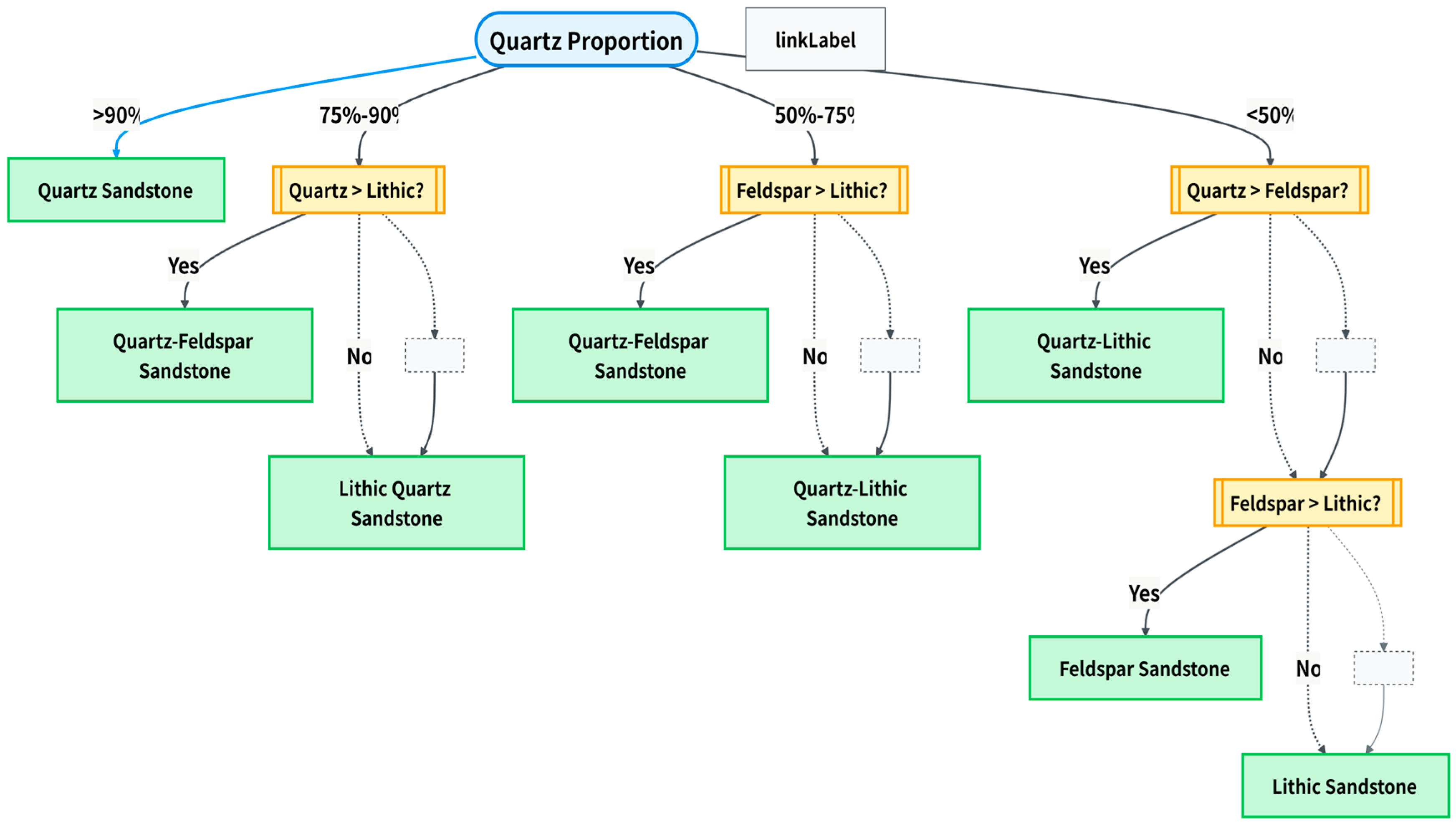
Naming of terrestrial source clastic components (NameTcc):

• Naming basis: based on the area proportion of various grains (quartz, feldspar, cuttings).
• Rule logic diagram (Figure 5):

2.

Integrated rock nomenclature (Name):

• Naming basis: grain size name + terrestrial clastic component name;
• Grain size classification criteria (

  Table 3. Grain size classification table.

  Grain Size Range (mm)	Φ Value Range	Grain Size Name
  >2	<−1	Conglomerate
  0.0625–2	4–0	Sandstone
  0.0039–0.0625	8–4	Siltstone
  <0.0039	>8	Mudstone

  ).

3.

A typical example:

• Main grain size: 0.25 mm (φ = 2) → Medium Sandstone;
• Component name: Feldspar Quartz Sandstone;
• Final name: Medium Feldspar Quartz Sandstone.

3. Materials and Experimental Analysis

3.1. Environment and Materials Preparation

1.

Environment: NVIDIA RTX3090 GPU + Intel Core i5-12490f CPU + 32GB Memory + Windows10 Operating System

2.

Dateset:

• The micrographs of tight sandstone used in this research were provided by the Oil and Gas Accumulation Laboratory of Sinopec.
• This study constructs a sandstone image dataset derived from diverse sources, encompassing core and outcrop samples from multiple critical petroliferous regions, including the Ordos Basin (Hangjinqi and Linxing areas), Tarim Basin (Taxi area), and Bohai Bay Basin (Bozhong Sag). Approximately half of the data were acquired from research projects and laboratory tests, covering key sedimentary facies such as braided river deltas and fan deltas, which represent typical reservoir facies like tight sandstone and marine sandstone. The other half were meticulously selected from the Rock Micro-image Thematic Database of the China Scientific Data platform, further enriching the diversity of compositional and textural characteristics. Overall, the image features exhibit both comprehensiveness and representativeness, thereby ensuring that our intelligent analysis models possess enhanced geological relevance and practical predictive capability.
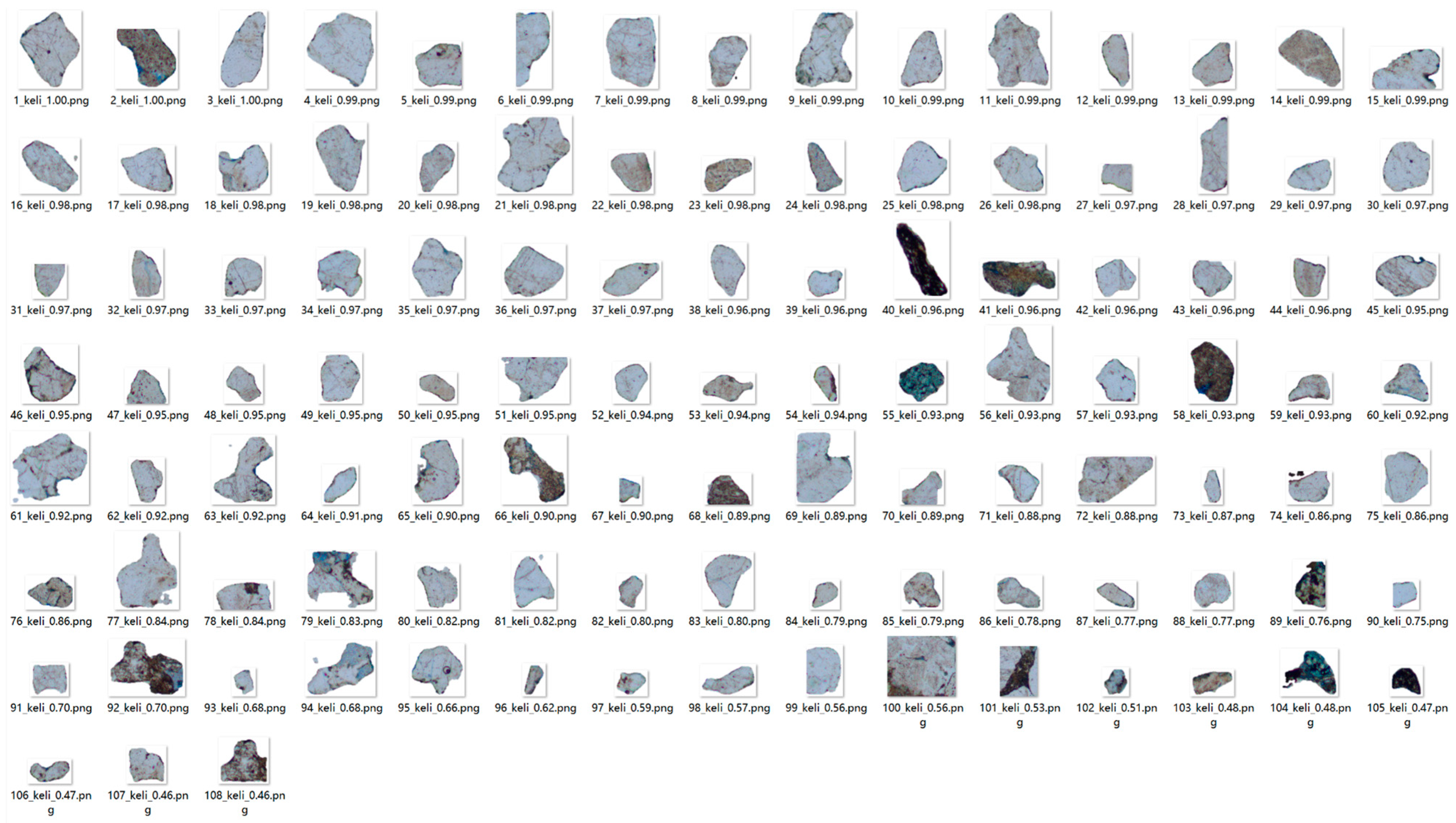
• The process of rock category annotation is to circle the rock grains with polygons formed by points and label them, and then extract the labeled substances in the annotated dataset. According to the polygon contour area of the labeled substances, a single image is cut out, as shown in Figure 6.
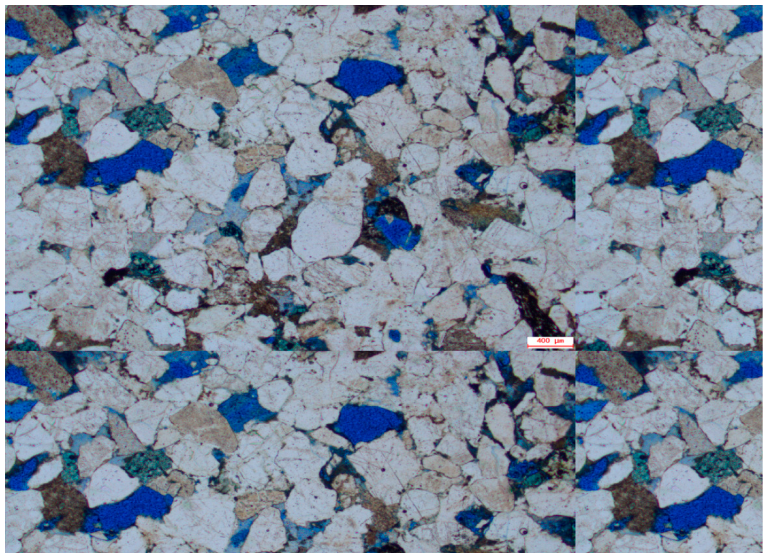
• At present, this system has labeled more than 800 images and more than 81,000 grains, forming a dataset of a certain scale: segmentation dataset SMISD and recognition dataset SMIRD [28,29]. In addition, the image rotation method is also used for data enhancement during the training process, as shown in Figure 7 (where the green grains in each figure are the same grain).
• To ensure the reliability and consistency of the annotated data, a rigorous verification protocol was implemented, comprising multi-annotator independent labeling, cross-validation, and expert review. Three specialists proficient in rock thin-section identification independently annotated a representative subset of 200 images (approximately 25% of the total dataset) using AnyLabeling software, in strict accordance with unified guidelines derived from the SY/T 5368-2016 industry standard. Consistency was quantitatively assessed using Intersection over Union (IoU) for grain boundary delineation (yielding an average IoU ≥ 0.85) and Cohen’s Kappa coefficient for mineral categorization (Kappa ≥ 0.82), reflecting substantial to near-perfect inter-annotator agreement. Instances of discrepancy (IoU < 0.7 or categorical mismatch, accounting for 5.3% of the subset) were referred to a senior geologist for arbitration and final resolution. Additionally, throughout data augmentation procedures—such as rotation and flipping—specific measures were enforced to maintain semantic accuracy in the annotations and avoid the introduction of biases. The finalized annotation consistency achieved for the constructed SMISD and SMIRD datasets reached 91.7%, satisfying the high-quality threshold necessary for robust deep learning model training.

3.

Key dependencies and hyperparameters:

• In order to ensure the reproducibility of the experiment, this system adopts a unified training framework, and the key dependencies and hyperparameter settings are shown in

  Table 4. The table of the dependent library package for the experiment.

  Dependent Packages	Version
  transformers	4.28.1
  matplotlib	3.5.1
  numpy	1.23.0
  opencv-python	4.7.0.72
  pandas	1.5.3
  scikit-learn	1.3.0
  torch	2.0.1 + cu118

  ,

  Table 5. Segmentation module training parameter configuration.

  Parameter Category	Parameter Setting	Illustration
  Optimizer	SGD	Kinetic energy = 0.9, weight decay = 10−4
  Initial learning rate	0.001	Cosine annealing scheduling (T_max = 100)
  Batch size	2	High-resolution image memory optimization
  Number of training rounds	50	Early termination mechanism (patience = 15)
  Mixing precision training	AMP start using	Accelerate training and reduce video memory usage

  and

  Table 6. Identification module training parameter configuration.

  Parameter Category	Parameter Setting	Illustration
  Optimizer	AdamW	ε = 10−8, β = (0.965,0.99)
  Initial learning rate	10−3	Cosine scheduling (warmup = 5 rounds)
  Batch size	160	Massively parallel processing
  Number of training rounds	60	Fixed rotation training
  Mixing precision training	AMP start using	Accelerate training and reduce video memory usage
  label smoothing	0.1	Mitigate overfitting
  Data augmentation	AutoAugment(‘rand-m9-mstd0.5-inc1’), MixUp(α = 0.8) + CutMix(α = 1.0), Random erase (probability 0.25)	Auto-enhancement/ Hybrid enhancement/Simulated occlusion scenario

  .

3.2. Experimental Analysis

In the SMISD dataset, the improved Mask R-CNN segmentation model adopts the dual-polarized light input strategy and adds a loss function for boundary optimization. The ablation experiment results corresponding to the structure are shown in

Table 7. Ablation experiments on the Mask R-CNN model with improved loss on the SMISD dataset.

Experimental Group	mIoU (%)	mAP@0.5 (%)	Border Misjudgment Rate (%)	Key Findings
Our system (Dual-polarized light + Improved Loss)	92.1	90.3	3.8	Optimal boundary segmentation (Shown in Figure 11)
Single-polarized light + Improved Loss	87.5/↓4.6	85.1/↓5.2	11.2/↑7.4	More missing grain segmentation of rock debris (Similar to Figure 2b)
Double-polarized light + Standard Loss	88.9/↓3.2	86.7/↓3.6	8.3/↑4.5	Blurred boundary (See Figure 2a for repeated segmentation)
Single-polarized light + Standard Loss	84.3/↓7.8	82.5/↓7.8	14.7/↑10.9	The dual problems of missing rock fragments and blurred boundary

.

During the training process, the loss function of the improved MetaFormer model gradually decreased while the precision rate steadily increased. After 128 epochs of training, the model demonstrated excellent convergence performance. This indicates that the model effectively learned the characteristics of sandstone microscopic images during training and progressively optimized its parameters to better adapt to identification tasks. On the test set, the model achieved a precision rate of 90.41%, with recall rates and F1 scores also showing outstanding performance. These results demonstrate that the enhanced MetaFormer model exhibits high recognition capability and segmentation accuracy in sandstone microscopic image analysis, effectively identifying mineral grains such as feldspar, debris, and quartz. These outcomes further validate that our improved MetaFormer model maintains high segmentation accuracy and robustness when processing various types of sandstone mineral grains. The performance of our Enhanced MetaFormer model is shown in

Table 8. Performance of MetaFormer model on SMIRD dataset.

Component	Precision	Recall	F1-Score
Quartz	91.2%	90.5%	90.8%
Debris	89.7%	88.9%	89.3%
Feldspar	90.5%	90.1%	90.3%

.

The enhanced MetaFormer recognition model utilizes a random hierarchical sampling strategy at a ratio of 4:1. To improve robustness and generalization, the model is trained using augmented data, while the test set remains composed of original particle images. The outcomes of the ablation experiments on data augmentation are summarized in

Table 9. SMIRD dataset training set data enhancement effect.

Data Size	Our Method (Random Affine Transformation + Flip + Gaussian Blur)	Traditional Method (Cropping + Color Distortion)	Gain
20,000	78.42%	56.78%	+21.64%
40,000	86.32%	62.45%	+23.87%
80,000	90.65%	65.12%	+25.53%

.

The enhanced MetaFormer recognition model incorporates a hybrid token mixer architecture composed of deep separable convolutions/pooling layers/mixed components at a CGA ratio of 4:4:4. Comparative analysis with mainstream classification models [30,31,32] and MetaFormer variants employing alternate token mixers—specifically a 6:6 CGA pooled mixer versus 6:6 CGA convolution-based mixer—is presented in Figure 8.

In Figure 8, the “Proposed System” model, depicted on the rightmost side of the chart, achieves the highest accuracy rates—92.78% on ImageNet and 90.65% on the SMIRD cross-polarization dataset—outperforming other models by approximately four percentage points. The results indicate that this performance advantage stems primarily from the synergistic effects of its hybrid architecture.

As shown in

Table 10. Hybrid Framework vs. Mask R-CNN Baseline Performance Comparison.

Assessment Indicators	Mask R-CNN Benchmark	Hybrid Framework (SAM + Mask R-CNN+ Enhanced MetaFormer)	Gain
mIoU (%)	84.3	92.1	↑7.8%
Boundary misjudgment rate (%)	14.7	3.8	↓10.9%
Identification rate of mineral components (%)	74.9	90.65	↑15.75%
Porosity measurement deviation (%)	±2.1	±0.3	↓85.7%

, the proposed system demonstrates a comprehensive performance breakthrough compared to the standard Mask R-CNN benchmark. This improvement is achieved by integrating the zero-shot segmentation capability of SAM with an enhanced two-stage segmentation and recognition architecture based on MetaFormer.

4. Results and Visualization

4.1. Segmentation Module Outputs

Plane-Polarized Light image of sandstone sub-image (Sample X53-1693.45m1-, as shown in Figure 9): Blue areas denote solvent-filled pore spaces, with remaining detrital grains requiring segmentation. All segmented grains derived from a single sub-image are displayed in Figure 10.

Segmentation overlay demonstration (Figure 11): Blue regions indicate solvent-filled voids, green zones represent segmented grains. The PPL and XPL images of the yellow particles used for demonstration are shown in Figure 12.

4.2. Identification Module Outputs

Quantification outputs in post-segmentation JSON files are as follows:

1.

{

2.

   "version": "4.5.6",

3.

   "flags": {},

4.

   "shapes": [

5.

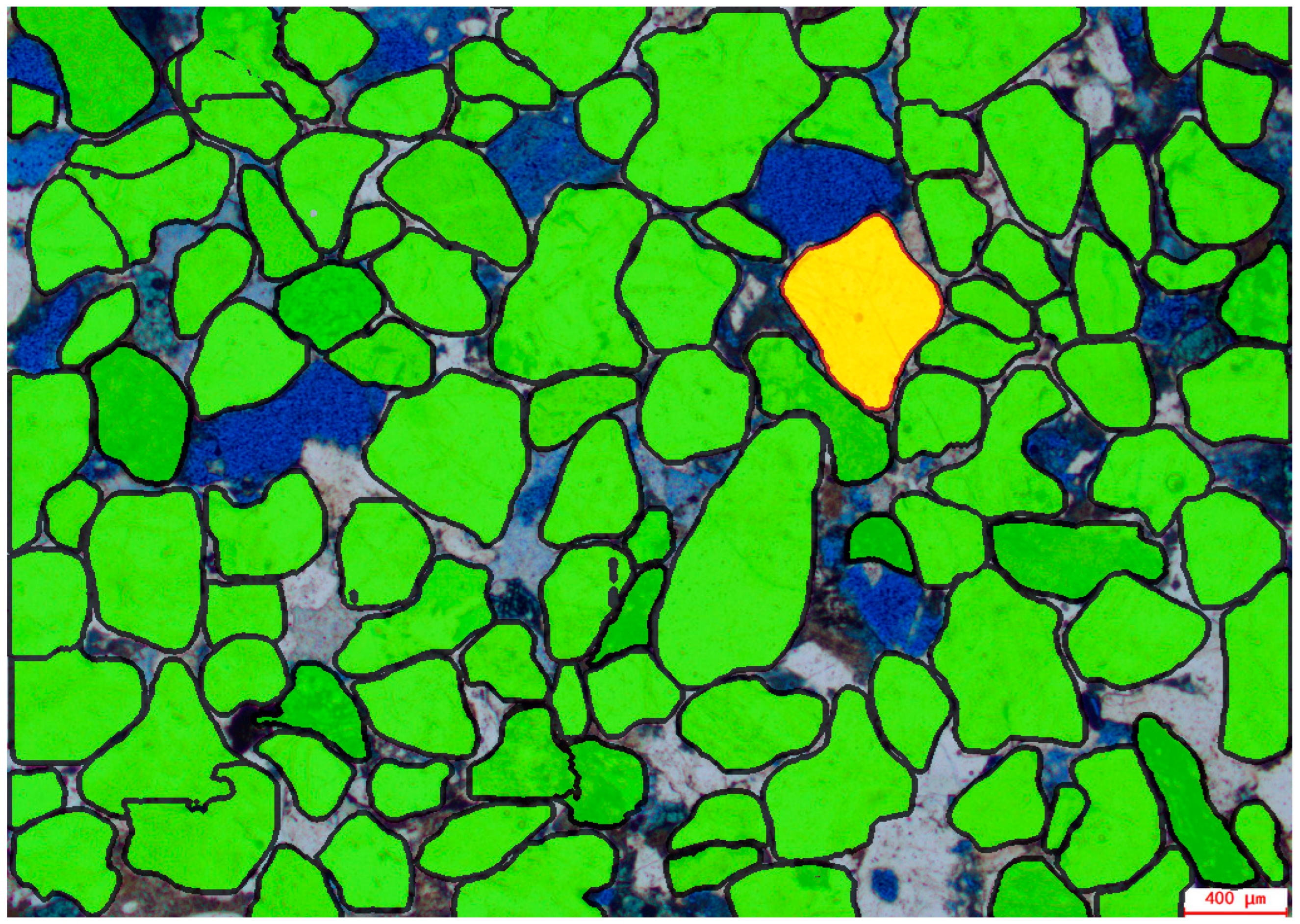
   # Identification parameters and boundary coordinate array of the initial segmented grain (pseudocolor yellow, Figure 11).

6.

    {

7.

     "label": "\u77f3\u82f1",

8.

     "points": [[690.0, 178.0], …], # The verticesarray contains polygon boundary coordinates, e.g., [690.0, 178.0].

9.

     "bbox": [ 616.0, 178.0, 746.0, 341.0], # Minimum circumscribed rectangle of grain entity, enabling rapid spatial indexing.

10.

     "shape_type": "polygon", # Shape annotation designated as polygonal boundaries.

11.

     "score": 0.9984123706817627 # Confidence metrics for geological feature detection.

12.

    }, …

13.

   # Remaining detrital grains exhibit analogous segmentation parameters without further elaboration.

14.

   ],

15.

   "imagePath": "X53-1693.45m1-.png",

16.

   "imageHeight": 1024,

17.

   "imageWidth": 768

18.

}

4.3. Morphometric Analysis Module Outputs

Graphical representations derived from morphological parameter calculations include the following.

1.

Figure 13 presents a bar chart showing roundness distribution across granulometric classes. Mean particle roundness indices per grain-size fraction are calculated from area/frequency tables of 12 discrete granulometric intervals. The x-axis denotes Udden–Wentworth grain-size classifications (e.g., Fine Sand, Medium Sand), while the y-axis represents particle roundness indices (dimensionless scale: 0–1.00).

2.

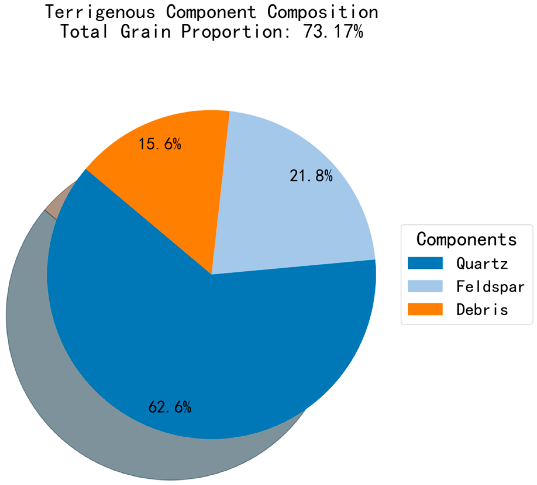
Figure 14 presents a pie chart illustrating relative abundance of terrigenous detrital components.

3.

Figure 15 presents a detrital grain size distribution pie chart. This visualization is derived from area/frequency tables across twelve granulometric intervals within the grain-size analysis framework.

4.

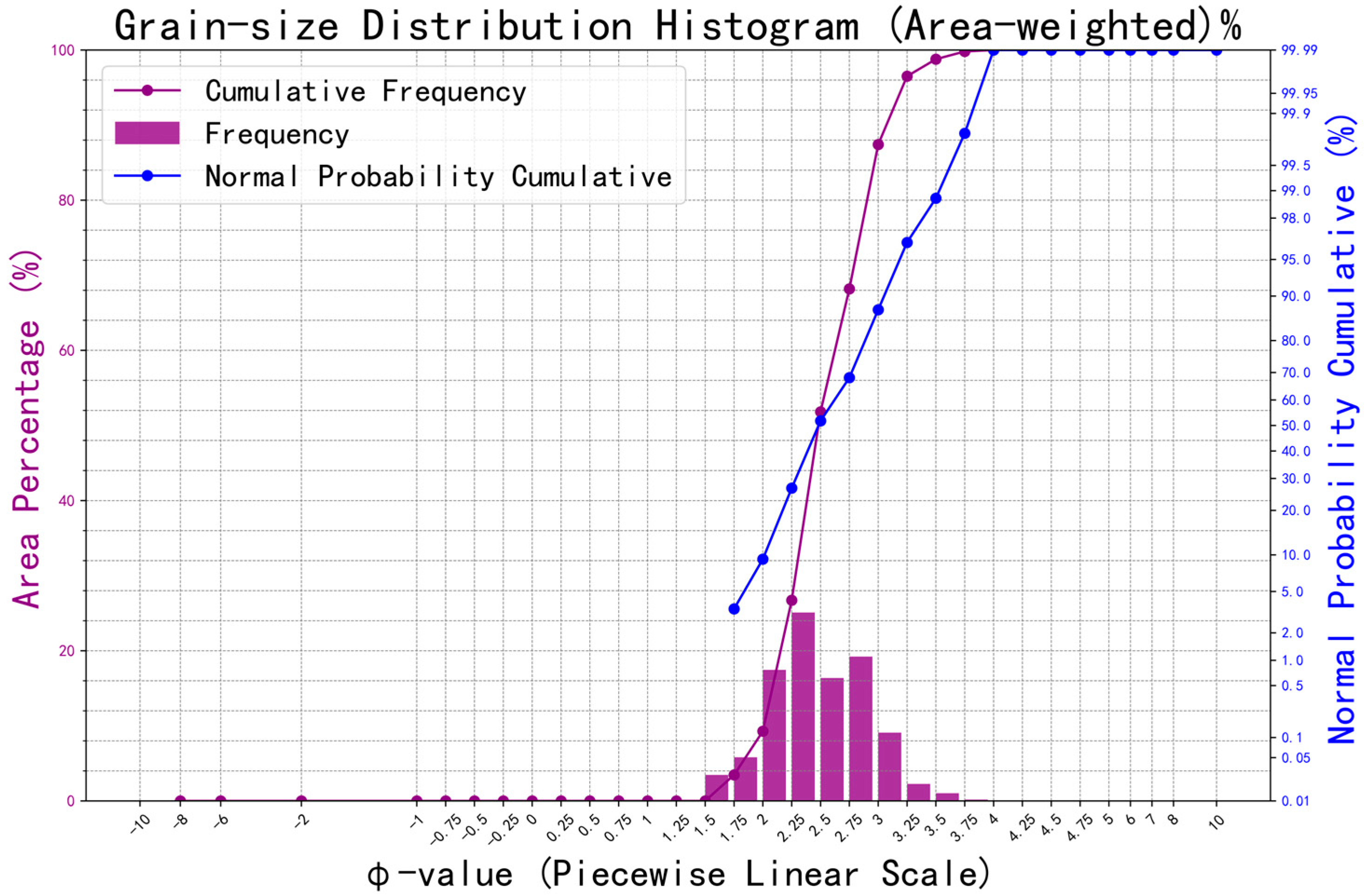
Figure 16 presents a tripartite grain size distribution plot integrating three graphical representations as follows:

• Frequency distribution histogram with φ-scale granulometric intervals on the x-axis and areal percentage per fraction on the y-axis;
• Cumulative frequency curve sharing identical φ-scale x-axis with cumulative areal percentage ordinate;
• Normal probability cumulative plot maintaining φ-scale abscissa while displaying probability percentage values.

5.

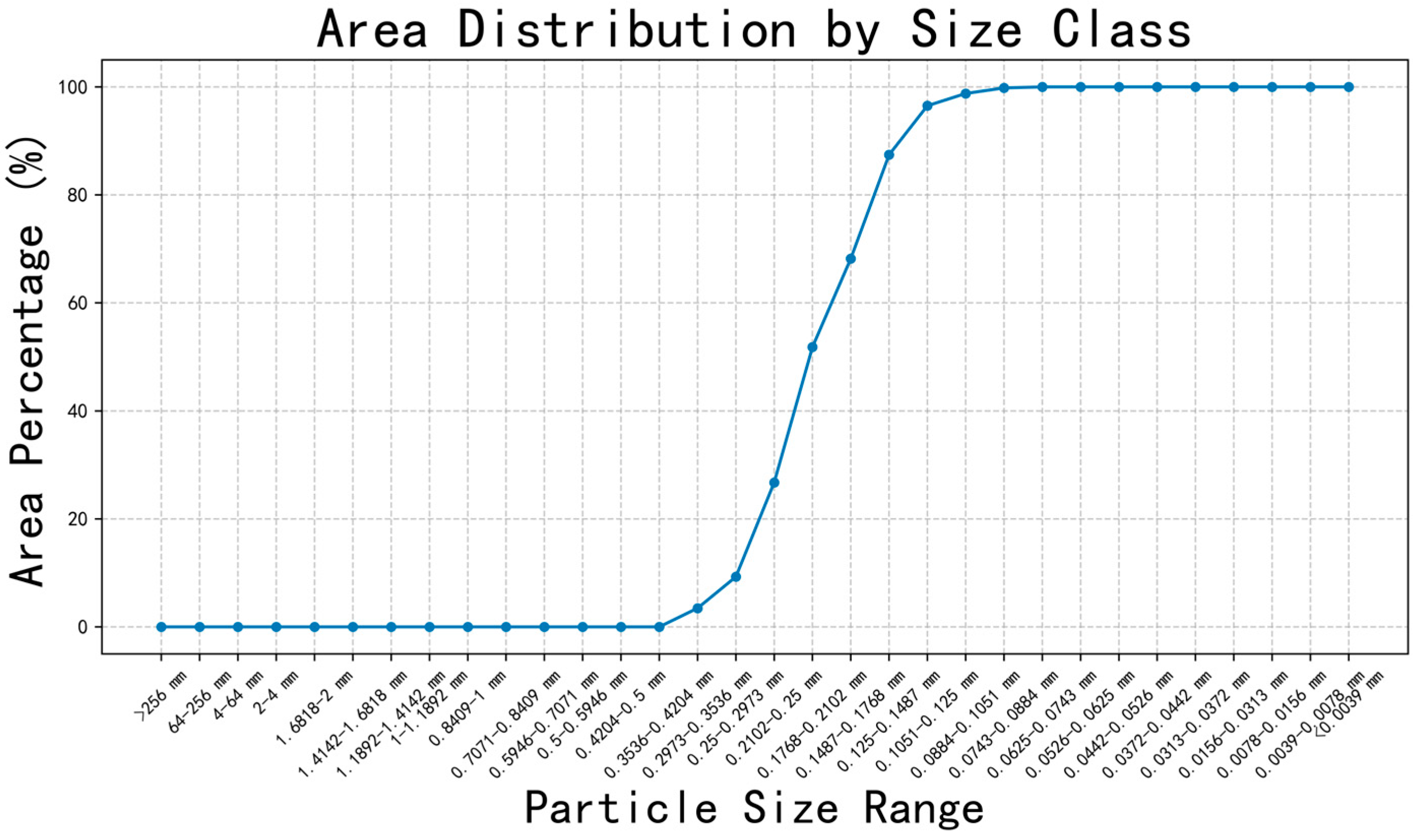
Figure 17 presents a line plot of areal distribution across granulometric classes employing identical methodology to the cumulative frequency plot within the tripartite grain size analysis, substituting phi (φ) values with absolute grain size ranges along the abscissa.

Post-calculation, the generated X53-1693.45m1-result.json file containing morphological parameters includes the following:

1.

{

2.

"Roundness": [ ‘……’ ], # Roundness indices list quantifying angularity for all grains

3.

"Rdstype": [ ‘……’ ], # Roundness classification list (0-4 scale: e.g., angular, subangular)

4.

"RdAreaSum": [ ‘……’ ], # Total areal coverage per roundness class (scale-converted)

5.

"RdPercentage": [ ‘……’ ], # Areal percentage per roundness class relative to total grain area

6.

"RdResult": "Angular and Subangular", # Dominant roundness types (highest-combined percentage classes)

7.

"MaximumGrainSize": 0.42, # Maximum grain diameter (mm)

8.

"MaximumGrainSizeTypeφ": 1.511264044967257, # φ-equivalent of maximum grain size

9.

"MainSizeRange": "No Statistically Dominant Grain-Size Fraction", # Primary granulometric distribution interval

10.

"SizePercentage": [ ‘……’ ], # Volumetric percentage per sieve-grade fraction (10-class)

11.

"AccPercentage": [ ‘……’ ], # Cumulative volumetric percentage per fraction (10-class)

12.

"SizePercentage32types": [ ‘……’ ], # Areal percentage per fraction (32-class)

13.

"CumFrequency32types": [ ‘……’ ], # Cumulative areal percentage per fraction (32-class)

14.

"StandardDeviation": 0.4258, # Graphic standard deviation (measure of distribution dispersion)

15.

"S0": 1.53, # Sorting coefficient (lower values = better sorting)

16.

"Mz": 2.51, # Graphic mean grain size (overall coarseness indicator)

17.

"Sk1": 0.0731, # Graphic skewness (distribution asymmetry: + = fine-skewed, - = coarse-skewed)

18.

"Kg": 0.9305, # Graphic kurtosis (distribution peakedness)

19.

"Cvalue": 0.3363, # C-value parameter (sedimentary environment discriminator)

20.

"Mvalue": 0.179, # M-value parameter (sedimentary environment discriminator)

21.

"MzMoment": 2.5153, # Moment measure mean grain size

22.

"SDMoment": 0.421, # Moment measure standard deviation

23.

"Sk1Moment": 0.0358, # Moment measure skewness

24.

"KgMoment": 2.9268, # Moment measure kurtosis

25.

"FractionResult": "well", # Sorting evaluation (e.g., "well"/"moderate"/"poor")

26.

"TotalDebris": 73.17, # Terrigenous component percentage of total sample

27.

"GrainPercentage": [62.56, 21.79,15.65], # Relative percentages of grain types within terrigenous fraction

28.

"NameTcc": "Lithic Feldspar Sandstone", # Lithological classification based on ternary components (e.g., "Lithic Feldspar Sandstone")

29.

"Name": "Medium Lithic Feldspar Sandstone", # Comprehensive lithological name incorporating granulometry (e.g., "Medium Lithic Feldspar Sandstone")

30.

"total_contacts": 174, # Total grain-grain contacts (for thin-section reconstruction)

31.

"Contact_percentage": { "No contact": 10.92, "Point contact": 52.87, "Concavo-convex contact": 36.21 }, # Percentage distribution of contact types

32.

"Dominant_contact_type": ["Point contact", 52.87], # Prevalent contact type and percentage

33.

"labels": [ ‘……’ ], # Mineralogical classifications (e.g., quartz, feldspar) for reconstruction matching

34.

"diameters": [ ‘……’ ], # Grain diameters (φ-scale)

35.

"perimeters": [ ‘……’ ], # Grain perimeters (scale-converted)

36.

"areas": [ ‘……’ ], # Grain areas (scale-converted)

37.

"img_size": 786432 # Image pixel dimensions (for reconstruction scaling)

38.

}

Pore Geometry Parameters in X53-1693.45m1-pore_annotation.json (Treating Pores as Particulate Entities):

1.

{

2.

  "version": "4.5.6",

3.

  "shapes": [

4.

    {

5.

     "label": "Pores",

6.

     "points": [[480, 736], [458, 741], [479, 752]],

7.

     "shape_type": "polygon"

8.

    }, …

9.

   # Remaining solvent-filled pores exhibit analogous morphometric quantification parameters without further elaboration.

10.

   ],

11.

   "imagePath": "X53-1693.45m1-.png",

12.

   "imageHeight": 1024,

13.

   "imageWidth": 768

14.

}

X53-1693.45m1-ArealPorosity_PoreDiameter.json storing quantitative metrics for pore systems:

1.

{

2.

   "porosity": 9.44, # porosity

3.

   "pore_diameters": [

4.

    21.17, 36.77, 19.75, 27.01, 24.72, 22.27, 20.44, 36.93, 29.58, 31.48, 37.44, 25.31, 25.33, 22.69, 20.23, 22.24, 87.39, 56.0, 31.98, 58.81, 54.79, 60.13, 114.65, 21.34, 19.75, 53.17, 64.8, 26.67, 27.58, 55.69, 21.47, 22.97, 39.84, 25.57, 27.63, 28.45, 21.89, 103.9, 44.19, 51.65, 84.13, 8.24, 29.27, 21.72, 1.36, 48.61, 61.05, 78.93, 55.32

5.

   ] # Equivalent Pore Diameter List

6.

}

5. Discussion

The hybrid system proposed in this study innovates in two aspects, surpassing the single application of the existing Mask R-CNN.

1.

Synergistic mechanism innovation between SAM and Mask R-CNN

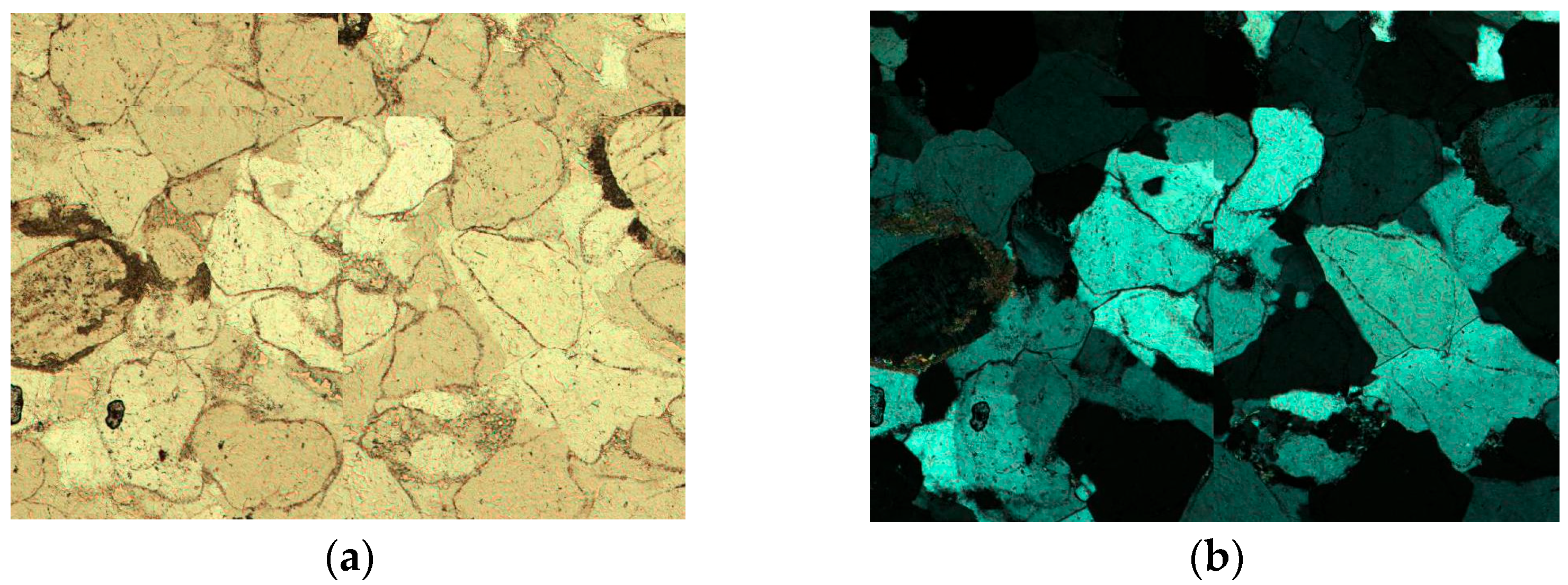
• Through SAM’s zero-sample pre-segmentation to generate dual-polarization light-guided annotation (Figure 3), combined with an improved Mask R-CNN boundary optimization loss function (Formula 2), we achieve for the first time a reduced quartz particle segmentation error rate from 12% to 3.8% (Table 5) and decreased cuttings particle missed segmentation rate by 7.4% (Compared with Ablation 1).
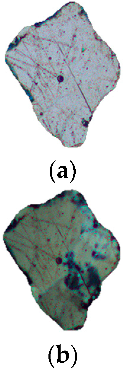
• Core innovation: Establishing a closed-loop “pre-segmentation/correction/precision segmentation” mechanism to resolve boundary ambiguity issues caused by mineral spectral overlap in traditional methods (Figure 2).

2.

MetaFormer cascaded token mixer architecture

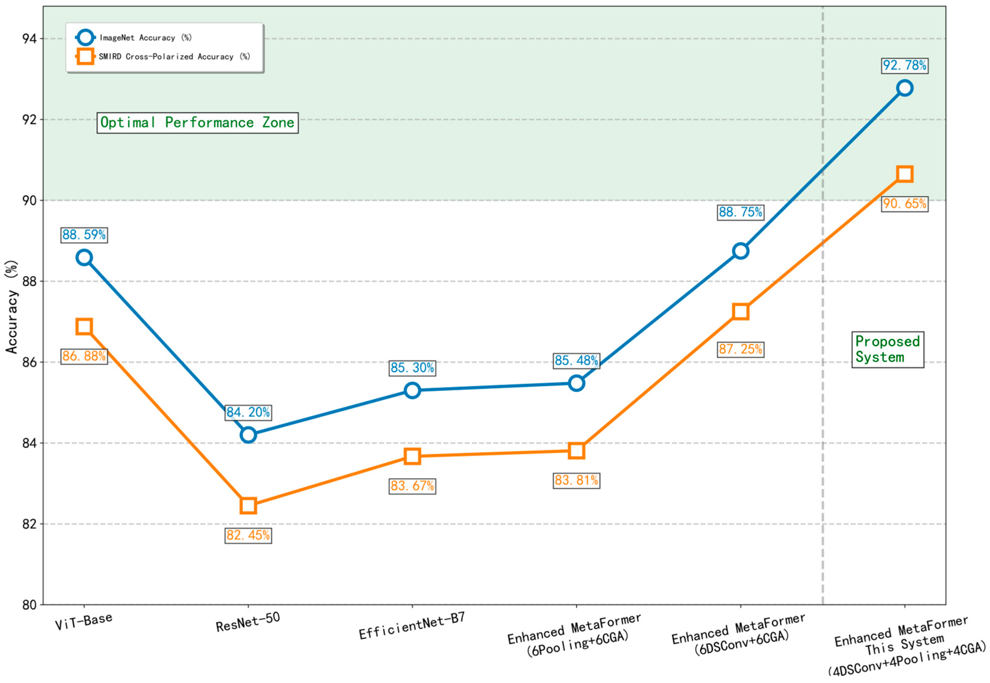
• Pioneering a three-stage cascade structure combining DSConv (local features), Hybrid Pooling (multi-scale features), and CGA (global attention) (Figure 4), achieved 90.65% mineral recognition accuracy on the SMIRD dataset (Table 6) and reduced FLOPs by 71% while increasing inference speed by 52% (Table 1).
• Core innovation: Overcoming the MSA redundancy bottleneck in traditional Transformers and achieving cross-modal fusion of mineral spectral features and morphological characteristics for the first time.

Furthermore, our subsequent GeoParam quantification module has established a new benchmark for lithology analysis by replacing the subjective Krummenberg classification method with topological indicators. Our porosity measurement deviation rate surpasses the ±5% industry tolerance limit specified in SPE 21048 standard, while the contact relationship classification system successfully resolves the long-standing challenge of cementation determination in traditional automated systems. These technological breakthroughs directly fill the “structural feature deficiency” gap identified by Liu et al. [3] in computational petrology research.

The proposed system demonstrates robust performance in bulk mineral identification (90.65% accuracy) but faces inherent constraints rooted in optical physics and data characteristics. Mineralogical discrimination limitations arise from spectral overlap under polarized light, particularly for feldspar subtypes (e.g., albite vs. K-feldspar), which require cathodoluminescence (CL) zoning pattern resolution. Nano-scale structural constraints prevent detection of sub-micron pores (<1 μm) due to the optical diffraction barrier (~0.2 μm), necessitating SEM-AM quantification for accurate characterization. Additionally, data-driven challenges emerge from skeletal grain class imbalance (quartz dominance causing a 12.3% lithic fragment accuracy drop) and unaddressed imaging condition variations—particularly the absence of stained thin-section training data, which elevates calcite cement misclassification by 22% under alizarin-red interference. Authigenic clay cement identification further requires SEM-EDS elemental mapping due to isotropic optical properties.

To transcend these limitations, we propose a three-mode verification ecosystem that could be implemented and work in the future.

1.

Optical-CL-SEM tiered workflow:

• Optical screening for rapid bulk mineralogy (<2 min/sample);
• CL verification for feldspar subtype/zoning analysis;
• SEM-AM nano-pore/cement quantification.

2.

Data-centric augmentation:

• GAN-synthesized stained/non-stained image pairs to bridge spectral gaps;
• Strategic oversampling of rare minerals (e.g., glauconite, heavy minerals).

3.

Algorithmic robustness engineering:

• Stain-invariant networks with spectral unmixing modules;
• Adversarial training for illumination/magnification invariance.

6. Conclusions

This research makes significant and measurable progress in intelligent sandstone analysis, with key contributions and implications as follows.

1.

Primary research contributions:

• A novel hybrid recognition framework was developed that effectively balances mineral identification accuracy with computational efficiency, providing a scalable solution for automated petrological analysis.
• An end-to-end workflow significantly reduces analysis time per sample from over 30 min to under 2 min while maintaining verifiable measurement precision, demonstrating strong potential for operational deployment.

2.

Implications and applications:

The methodology offers an immediately applicable tool for reservoir characterization in standard laboratory environments, with particular value in high-throughput industrial and research settings. By reducing reliance on subjective manual interpretation, this system enhances the consistency and comparability of petrological data across studies.

3.

Future directions:

While the system shows considerable promise, further validation across diverse geological settings is essential to confirm its broad applicability. This framework provides efficient tight sandstone screening but still has inherent optical constraints. Future work will integrate optical-CL-SEM tri-modal fusion to transcend single-technique limits. Subsequent development will focus on extending the system’s capability to complex mineral assemblages via multimodal data fusion, thereby widening its utility within geoscience and engineering applications.

References

- Al-Amri, S.S.; Kalyankar, N.V. Image segmentation by using threshold techniques. arXiv 2010, arXiv:1005.4020. [Google Scholar] [CrossRef]
- Muñoz, X.; Freixenet, J.; Cufí, X.; Martı, J. Strategies for image segmentation combining region and boundary information. Pattern Recogn. Lett. 2003, 24, 375–392. [Google Scholar] [CrossRef]
- Muthukrishnan, R.; Radha, M. Edge detection techniques for image segmentation. Int. J. Comput. Sci. Inf. Technol. 2011, 3, 259. [Google Scholar] [CrossRef]
- Peng, B.; Zhang, L.; Zhang, D. A survey of graph theoretical approaches to image segmentation. Pattern Recogn. 2013, 46, 1020–1038. [Google Scholar] [CrossRef]
- Zhou, Y.; Starkey, J.; Mansinha, L. Segmentation of petrographic images by integrating edge detection and region growing. Comput. Geosci. 2004, 30, 817–831. [Google Scholar] [CrossRef]
- Ross, B.J.; Fueten, F.; Yashkir, D.Y. Automatic mineral identification using genetic programming. Mach. Vis. Appl. 2001, 13, 61–69. [Google Scholar] [CrossRef][Green Version]
- Jiang, F.; Gu, Q.; Hao, H.; Li, N.; Wang, B.; Hu, X. A method for automatic grain segmentation of multi-angle cross-polarized microscopic images of sandstone. Comput. Geosci. 2018, 115, 143–153. [Google Scholar] [CrossRef]
- Zhang, Y.; Li, M.C.; Han, S. Automatic Lithology Identification and Classification Method Based on Rock Image Deep Learning. Acta Petrol. Sin. 2018, 34, 333–342. [Google Scholar]
- Szegedy, C.; Vanhoucke, V.; Ioffe, S.; Shlens, J.; Wojna, Z. Rethinking the Inception Architecture for Computer Vision. In Proceedings of the 2016 IEEE Conference on Computer Vision and Pattern Recognition (CVPR), Las Vegas, NV, USA, 27–30 June 2016; pp. 2818–2826. [Google Scholar]
- Liu, X.; Wang, H.; Jing, H.; Shao, A.; Wang, L. Research on Intelligent Identification of Rock Types Based on Faster R-CNN Method. IEEE Access 2020, 8, 21804–21812. [Google Scholar] [CrossRef]
- Ren, S.; He, K.; Girshick, R.; Sun, J. Faster R-CNN: Towards Real-Time Object Detection with Region Proposal Networks. IEEE Trans. Pattern Anal. Mach. Intelligence 2017, 39, 1137–1149. [Google Scholar] [CrossRef] [PubMed]
- Simonyan, K.; Zisserman, A. Very Deep Convolutional Networks for Large-Scale Image Recognition. In Proceedings of the International Conference on Learning Representations, San Diego, CA, USA, 7–9 May 2015. [Google Scholar]
- Hu, Q. Deep Learning Classification Method for Rock Thin-Section Images with Multi-Dimensional Information. Master’s Thesis, Zhejiang University, Hangzhou, China, 2019. [Google Scholar]
- Kirillov, A.; Mintun, E.; Ravi, N.; Mao, H.; Rolland, C.; Gustafson, L.; Xiao, T.; Whitehead, S.; Berg, A.C.; Lo, W.-Y.; et al. Segment Anything. In Proceedings of the IEEE/CVF International Conference on Computer Vision, Paris, France, 2–6 October 2023; pp. 4015–4026. [Google Scholar]
- He, K.; Gkioxari, G.; Dollár, P.; Girshick, R. Mask R-CNN. In Proceedings of the IEEE International Conference on Computer Vision, Venice, Italy, 22–29 October 2017; pp. 2961–2969. [Google Scholar]
- Yu, W.; Luo, M.; Zhou, P.; Si, C.; Zhou, Y.; Wang, X.; Feng, J.; Yan, S. MetaFormer Is Actually What You Need for Vision. In Proceedings of the IEEE/CVF Conference on Computer Vision and Pattern Recognition, New Orleans, LA, USA, 18–24 June 2022. [Google Scholar]
- Naseer, M.M.; Ranasinghe, K.; Khan, S.H.; Hayat, M.; Shahbaz Khan, F.; Yang, M.H. Intriguing Properties of Vision Transformers. Adv. Neural Inf. Process. Syst. 2021, 34, 23296–23308. [Google Scholar]
- Qin, D.; Leichner, C.; Delakis, M.; Fornoni, M.; Luo, S.; Yang, F.; Wang, W.; Banbury, C.; Ye, C.; Akin, B.; et al. MobileNetV4—Universal Models for the Mobile Ecosystem 2024. In European Conference on Computer Vision; Springer Nature: Cham, Switzerland, 2024. [Google Scholar]
- Liu, X.; Peng, H.; Zheng, N.; Yang, Y.; Hu, H.; Yuan, Y. EfficientViT: Memory Efficient Vision Transformer with Cascaded Group Attention. In Proceedings of the 2023 IEEE/CVF Conference on Computer Vision and Pattern Recognition (CVPR), Vancouver, BC, Canada, 17–24 June 2023; pp. 14420–14430. [Google Scholar]
- Folk, R.L.; Ward, W.C. A Study in the Significance of Grain-Size Parameters. J. Sediment. Petrol. 1957, 27, 3–26. [Google Scholar] [CrossRef]
- Cox, E.P. A Method of Assigning Numerical and Percentage Values to the Degree of Roundness of Sand Grains. J. Paleontol. 1927, 1, 179–183. [Google Scholar]
- SY/T 5368-2016; Identification of Rock Thin Sections. National Energy Administration: Beijing, China, 2016.
- SY/T 5434-2018; Analysis Method for Particle Size of Clastic Rocks. National Energy Administration: Beijing, China, 2018.
- Krumbein, W.C. Size Frequency Distribution of Sediments. J. Sediment. Res. 1934, 4, 65–77. [Google Scholar] [CrossRef]
- Shaanxi Team of Chengdu Geological College. Grain Size Analysis and Application of Sedimentary Rocks (Materials); Geological Publishing House: Beijing, China, 1978; pp. 1–29. [Google Scholar]
- Friedman, G.M. Distribution Between Dune, Beach, and River Sands from the Textural Characteristics. J. Sediment. Petrol. 1961, 31, 514–519. [Google Scholar]
- SY/T 6103-2019; Measurement of Rock Pore Structure—Image Analysis Method. National Energy Administration: Beijing, China, 2019.
- Gui, H. Key Technologies for Intelligent Analysis of Sandstone Micrographs. Master’s Thesis, University of Science and Technology of China, Hefei, China, 2022. [Google Scholar]
- Zhang, Z.Y. Research on Segmentation and Recognition of Sandstone Thin-Section Images. Master’s Thesis, University of Science and Technology of China, Hefei, China, 2020. [Google Scholar]
- Targ, S.; Almeida, D.; Lyman, K. Resnet in Resnet: Generalizing Residual Architectures. arXiv 2016, arXiv:1603.08029. [Google Scholar] [CrossRef]
- Tan, M.; Le, Q. EfficientNet: Rethinking Model Scaling for Convolutional Neural Networks. In Proceedings of the 36th International Conference on Machine Learning, Long Beach, CA, USA, 9–15 June 2019; pp. 6105–6114. [Google Scholar]
- Dosovitskiy, A.; Beyer, L.; Kolesnikov, A.; Zhai, X.; Unterthiner, T.; Dehghani, M.; Minderer, M.; Heigold, G.; Gelly, S.; Uszkoreit, J.; et al. An Image Is Worth 16 × 16 Words: Transformers for Image Recognition at Scale. arXiv 2020, arXiv:2010.11929. [Google Scholar]