Article

Yield Stress Prediction of Filling Slurry Based on Rheological Experiments and Machine Learning

Kunming Metallurgical Research Institute Co., Ltd., Kunming 650021, China
*
Authors to whom correspondence should be addressed.
Minerals 2025, 15(9), 931; https://doi.org/10.3390/min15090931
Submission received: 6 July 2025 / Revised: 24 August 2025 / Accepted: 25 August 2025 / Published: 1 September 2025

Abstract

Cemented filling technology is an effective approach to solving tailings accumulation and goaf, with rheological properties serving as key indicators of slurry fluidity. Since slurry rheology is influenced by multiple factors, accurate prediction of its parameters is essential for optimizing filling design. In this study, we developed a model to predict static and dynamic yield stress using the extreme gradient boosting (XGBoost) algorithm, trained on 140 experimental samples (105 for training and 35 for validation, split 75:25). For comparison, adaptive boosting tree (ADBT), gradient boosting decision tree (GBDT), and random forest (RF) algorithms were also applied. Model performance was evaluated using four metrics: coefficient of determination (R2), mean absolute error (MAE), root mean square error (RMSE), and explained variance score (EVS). The Shapley additive explanation (SHAP) method was employed to interpret model outputs. The results show that XGBoost achieved superior predictive accuracy for slurry yield stress compared with other models. Analysis of importance revealed that underflow concentration had the strongest influence on predictions, followed by the binder-to-tailings ratio, while the fine-to-coarse tailings ratio contributed least. These findings highlight the potential of machine learning as a powerful tool for modeling the rheological parameters of filling slurry, offering valuable guidance for engineering applications.

Graphical Abstract

1. Introduction

With the advancement of science and technology and the growing demand for mineral resources, global iron ore consumption has continued to increase [1]. As ore grades decline, enhanced recovery processes generate large volumes of fine tailings, whose long-term accumulation poses serious environmental and safety risks. These risks include geological hazards such as mudslides, groundwater contamination from heavy metals, and ecological degradation [2,3,4]. For example, the 2019 Brumadinho dam failure in Brazil resulted in 270 fatalities and severe river pollution [5]. In China, remediation of a vast number of tailings ponds has been identified as an urgent priority, as highlighted in the 2022 MIIT guidelines [6]. Such documented impacts underscore the need for innovative tailings management strategies.
Cemented filling technology provides an effective means of reusing tailings by transporting them underground to fill mined-out voids, thereby achieving the dual goal of waste disposal and ground support [7,8,9,10]. The process typically involves three steps: (1) thickening low-concentration tailings slurry to produce a high-concentration slurry, (2) preparing the filling slurry by mixing this concentrate with coarse aggregates, binders, and additives, and (3) transporting the slurry to the stope either by gravity or pumping [11,12]. Among these, the mixing stage is critical. A well-prepared slurry not only ensures good flowability but also produces a filling body with high compressive strength. Rheological parameters serve as macroscopic indicators of the slurry’s microstructural behavior and thus provide an essential basis for optimizing the mixing process [13,14,15].
Dynamic and static yield stress are two fundamental parameters that characterize the rheological behavior of filling slurries [16,17]. However, slurry rheology is influenced by many factors, and experimental observations are often case-specific, limiting their applicability across different tailings sources. Moreover, direct measurement of rheological parameters is both costly and time-consuming, making it difficult to integrate rheological testing into large-scale mining operations. Consequently, predictive approaches are vital for enabling practical applications of slurry rheology in cemented filling technology.
In recent years, predictive models have been increasingly applied to estimate the rheological and mechanical properties of filling slurries [18,19,20,21]. Since slurry properties are strongly dependent on material composition, conventional mathematical models are often restricted to specific material systems. Given the limited availability of experimental datasets, machine learning offers a promising alternative, capable of improving predictive accuracy and generalization. Previous studies have successfully linked unconfined compressive strength to mix composition [22,23,24] and established models mapping slurry composition to slump and compressive strength [25]. Various machine learning methods—including artificial neural networks, support vector machines, and random forests—have proven effective for such predictions [26,27,28,29]. For instance, Gomaa et al. [30] used random forests to predict the slump and compressive strength of fly ash-based concrete, while Nehdi and Al Martini [31] applied genetic algorithms to model the relationship between shear strain and shear stress in cement paste under different temperatures and shear conditions. Ensemble learning approaches, which integrate multiple models to leverage their complementary strengths, have further enhanced predictive accuracy. For example, Nguyen et al. [32] developed a hybrid model based on least squares support vector machines and particle swarm optimization to predict interface yield stress and plastic viscosity in concrete.
Among ensemble methods, extreme gradient boosting (XGBoost), proposed by Chen, has emerged as a particularly powerful tool [33]. XGBoost combines high computational efficiency with improved predictive accuracy [34,35].
This study develops an XGBoost-based predictive model for static and dynamic yield stress, trained on experimental data from 140 samples. The selected input features include underflow concentration, binder-to-tailings ratio, and fine-to-coarse tailings ratio, while the outputs are static and dynamic yield stresses. This study first describes the rheological experiments, then presents the machine learning methodology, compares XGBoost to alternative algorithms, and finally interprets the results using the Shapley additive explanation (SHAP) method. The framework of the XGBoost model is shown in Figure 1.

2. Experiments and Results

2.1. Materials and Experimental Procedures

The tailings used in this study were collected from an iron mine in China, and the binder was a specially formulated anhydrous gypsum cement. The filling slurry was prepared from fine tailings, coarse tailings, binder, and water. Prior to testing, the tailings were dried, cleaned, and crushed. The fine tailings were generated by a ball mill in a concentrator, while the coarse tailings were collected as the underflow from spiral classification.
The particle size distributions of the fine tailings and binder were analyzed using a laser particle size analyzer (Malvern Panalytical, Mastersizer 3000, Malvern Panalytical Ltd., Malvern, UK), as shown in Figure 2. The median particle size was 13.52 μm for the fine tailings and 11.2 μm for the binder. The particle size distribution of the coarse tailings is presented in Table 1. The densities were measured using a pycnometer: 2.898 g/cm3 for the tailings and 2.363 g/cm3 for the binder. Distilled water was used in all experiments.
The oxide compositions of the tailings and binder were determined by X-ray fluorescence spectroscopy (Thermo Fisher ARL Perform X4200W, Thermo Fisher Scientific Inc., Waltham, MA, USA) (Table 2). The tailings were rich in SiO2, followed by MgO, Fe2O3, and Al2O3, while the binder was primarily composed of CaO, SiO2, SO3, and Al2O3.

2.2. Experimental Setup

To evaluate the effects of key parameters on slurry rheology, experiments were conducted under varying fine-to-coarse tailings ratios, binder-to-tailings ratios, and underflow concentrations. Based on actual production conditions, the fine-to-coarse tailings ratio was set at four levels (9:1, 10:1, 11:1, and 12:1), and the binders–tailings ratio was set at seven levels (1:4, 1:6, 1:8, 1:10, 1:12, 1:14, and 0). Five levels of underflow concentration (measured in mass fraction) obtained in the thickening stage were set based on different fine-to-coarse tailings ratios. The fine–coarse tailings ratio was calculated as the mass ratio of fine tailings (ball mill output) to coarse tailings (spiral classifier underflow). The experimental conditions were shown in Table 3, and a total of 140 test sets were conducted.
Slurry samples were first mixed manually for 120 s, then transferred to a mechanical mixer and stirred at 65 r/min for an additional 120 s. Homogeneity was defined by the absence of visible agglomerates and variation of less than 5% across three replicate tests. All experiments were conducted at a controlled temperature of 25 ± 1 °C.
Rheological measurements were performed using a Brookfield RST rotary rheometer with a VT80-40 cross-paddle rotor (40 mm diameter, 80 mm height) in a stainless steel cylindrical container (inner diameter 130 mm, height 170 mm). The test program included both static yield stress and dynamic yield stress measurements (Figure 3). Research from Li et al. shows that setting the shear rate at around 0.3 s−1 can ensure that the slurry is not excessively damaged, and the static yield stress of the slurry can be obtained [36]. Therefore, the static yield stress experiment is carried out at a constant shear rate of 0.3 s−1 for 60 s to obtain a shear stress–time curve for the sample, with the static yield stress of the slurry as the peak point of the curve. At the same time, relevant studies have shown that steady-state shear stress under certain shear rate conditions can only be obtained when the slurry is sheared for more than 10 s [37,38]. The dynamic yield stress experiment is performed by decreasing from 80 s−1 to 10 s−1 in steps of 10 s−1, then shearing the slurry at shear rates of 5 s−1 and 1 s−1 for 10 s at each shear rate level to obtain a shear stress–shear rate curve for the sample. The shear rate is not set below 1 s−1, to reduce the influence of unsteady flow on the rheological parameters of filling slurry [39].

2.3. Experimental Results

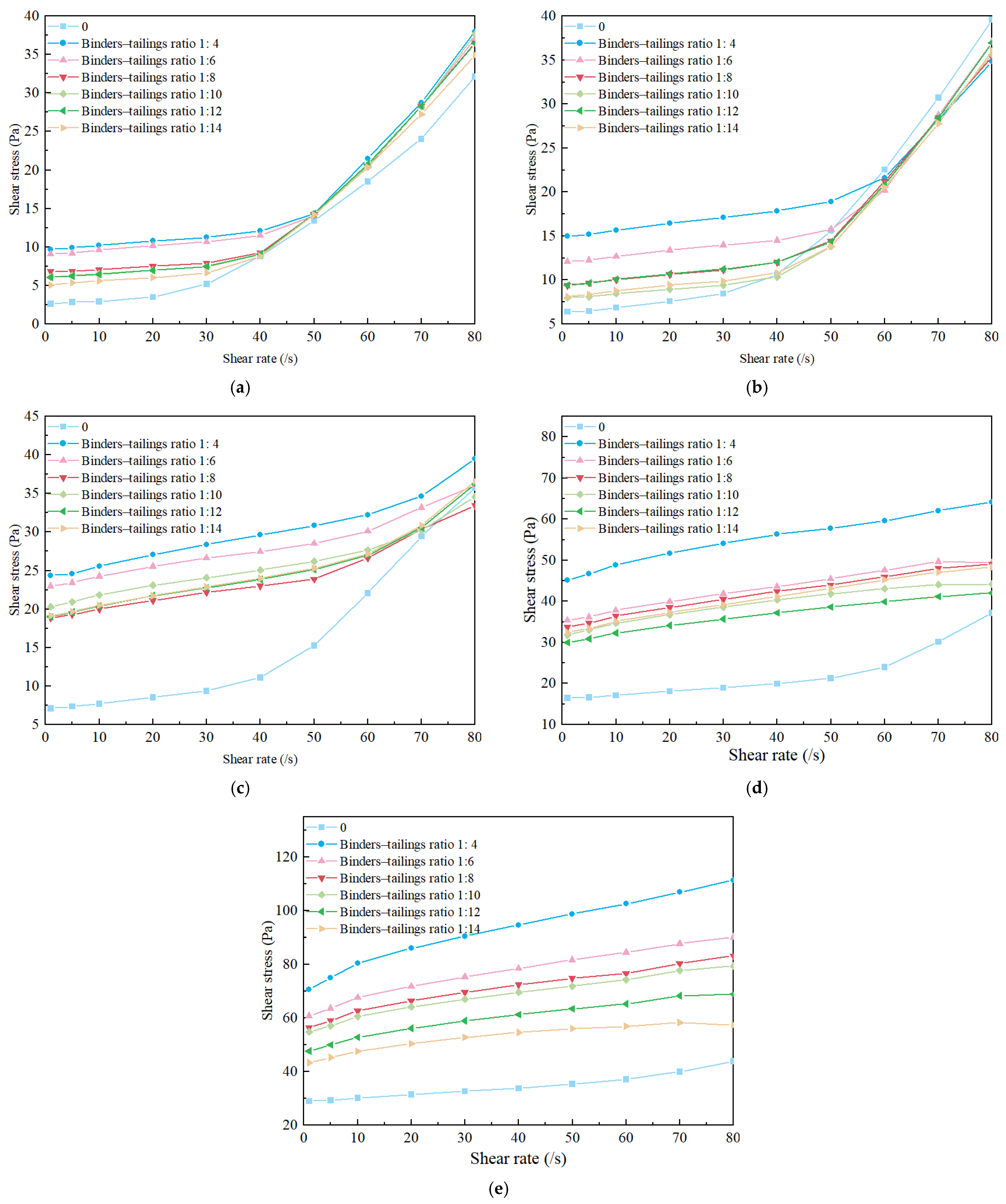
Figure 4 shows the flow curves of the slurry at a fine-to-coarse tailings ratio of 12:1. Shear stress increased with shear rate, confirming that the slurry behaved as a typical Herschel–Bulkley fluid. The dynamic yield stress was obtained by fitting the descending portion of the shear rate curve. Flow curves for other ratios (9:1, 10:1, 11:1) are provided in the Supplementary Materials.
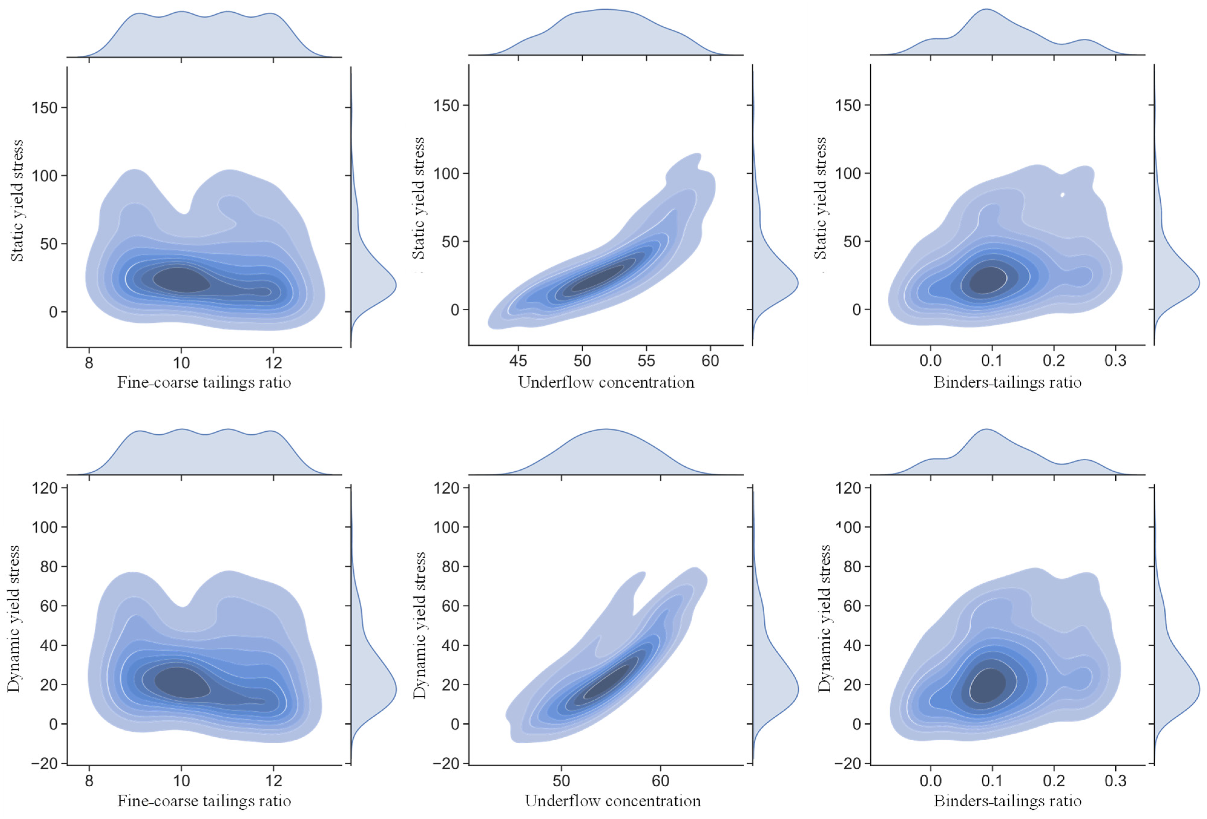
Three key input features—fine-to-coarse ratio, underflow concentration, and binder-to-tailings ratio—were selected for subsequent modeling. Figure 5 presents the distributions of experimental features and outputs. Both static and dynamic yield stresses exhibited strong correlations with the independent variables. Static yield stress consistently exceeded dynamic yield stress, consistent with theoretical expectations of slurry behavior.

3. Construction and Implementation of the Model

3.1. XGBoost Methodology

The predictive model was developed in Python (Anaconda, version 3.9.7) using the XGBoost algorithm to estimate static and dynamic yield stress. Unlike traditional decision trees, which follow a simple binary structure to arrive at terminal nodes, XGBoost is an ensemble method that integrates a sequence of decision trees. Each tree builds on the errors of the previous ones, progressively improving model accuracy [40].
Assume a dataset with independent variables xi each with b eigenvalues, where xiRm. Each independent variable corresponds to a dependent variable yi, where yiR. The prediction function of XGBoost can be expressed as
y ^ i = γ ( x i ) = k = 1 K f k ( x i ) ,   f k F
where y ^ i is the predicted value, fk represents the function corresponding to a decision tree, and F is the set of all possible regression trees.
Similar to other machine learning models, the prediction function of the XGBoost model includes a loss function and a canonical term, and the canonical term is respon-sible for measuring the complexity of the model. Equation (2) shows the objective func-tion to predict yield stress:
G = i E y i , y ^ i + k H f k
The training error of E sample xi in Equation (2) is the loss function, and the regu-larization term H, the canonical term, is calculated as
H f = γ T + 1 2 λ j ω j 2
where γ is the regular term coefficient for the complexity of each leaf, and T and ωi represent the number of leaves and the weight of the jth leaf, respectively.
The canonical term avoids overfitting, and the objective function prefers a simple model with predictive power. y ^ i t in the tth iteration is calculated as
y ^ i t = y ^ i ( t 1 ) + f t ( x i )
It can be seen that the tth iteration model consists of the t − 1st iteration model and a new sub-model f t ( x i ) . Therefore, in order to minimize the objective function G, an approximation method is used to optimize the objective function, and a Taylor second-order expansion of the objective function is obtained as
G ( t ) i = 1 n E ( y i , y ^ i ( t 1 ) ) + g i f t ( x i ) + 1 2 h i f t 2 ( x i ) + H ( f t )
where g i is the first-order derivative of E ( y i , y ^ i ( t 1 ) ) concerning y ^ i ( t 1 ) , and h i is the second-order derivative of E ( y i , y ^ i ( t 1 ) ) for y ^ i ( t 1 ) .
I j is defined as the set of samples at leaf node j, in which all samples fall on leaf node j. f t ( x i ) divides the sample into leaf nodes and calculates the score ω for that leaf node. When i I j , f t ( x i ) can be replaced by ω j . Equation (5) is simplified, and the partial derivative of ω j is taken, such that the partial derivative is zero. The minimum value of the preferred weight and objective function is
ω j * = i I j g i i I j h i + λ
M ( t ) = 1 2 j = 1 T i I j g i 2 i I j h i + λ + γ T
It is impossible to solve the above equations for all possible trees. XGBoost uses a greedy algorithm to obtain a more straightforward formulation. Assuming that IL and IR are the sample sets of the left and right child nodes after the split, I denotes the sample set of the node before splitting, where I = ILIR. The formula for the change of the objective function before and after the node split is shown in Equation (8):
M s p l i t = 1 2 i I L g i 2 i I L h i + λ + i I R g i 2 i I R h i + λ i I g i 2 i I h i + λ γ
When Msplit reaches the maximum, the splitting point is the most excellent splitting point, and the optimal integration model is eventually established after many repetitions.

3.2. Model Evaluation

In supervised learning, the entire dataset needs to be split into two subsets: a training set and a test set. The training set is used for model training and hyperparameter tuning, while the test set is used for performance evaluation. Drawing on relevant research [41], this paper analyzes and optimizes the split dataset. In this paper, 75% (105 samples) of the entire dataset was used as the training set, and the remaining 25% (35 samples) was used as the test set. Four evaluation metrics are selected to assess the adequacy and validity of the XGBoost model, including coefficient of determination (R2), mean absolute error (MAE), root mean square error (RMSE), and explained variance score (EVS), and the definition of each metric is shown in Table 4. The coefficient of determination (R2) quantifies the proportion of variance explained by the model, with values >0.9 indicating excellent fit. Mean absolute error (MAE) reflects the average magnitude of prediction errors, directly indicating engineering relevance. Root mean square error (RMSE) emphasizes larger errors due to its quadratic weighting, making it a key safety indicator in engineering contexts. Explained variance score (EVS) assesses robustness against input variations, where values > 0.9 confirm model stability under diverse mix designs.

3.3. Hyperparameter Tuning

The predictive accuracy of XGBoost is highly sensitive to hyperparameter settings. To avoid overfitting and maximize performance, systematic parameter optimization was performed. The learning rate “Eta” is an important parameter that can effectively prevent model overfitting and improve model robustness by reducing the weight of each step. The model usually divides nodes when the loss function is greater than 0. The parameter “gamma” gives the loss function required by the model, with larger values of “gamma” making the model more conservative. The parameter “subsample” describes the fraction of training model subsamples in collecting samples. “Colsample_bytree” characterizes the proportion of features that are randomly sampled when building the tree and takes a value between 0 and 1. “Min_child_weight” represents the minimum number of samples needed to construct each model. The parameters “lambda” and “alpha” are the L2 and L1 regularization terms, respectively, which are added to make the model more robust. “Max_depth” is the maximum depth of the tree, indicating the maximum number of splits. Increasing the maximum depth is more likely to lead to overfitting.
Parameter tuning entails giving initial values to some of the parameters and then adjusting the tuning parameters one by one until the model is optimal. The criterion for parameter tuning is based on RMSE minimization. The learning rate is determined at first, which generally fluctuates in the range of 0.05–0.3; for a given learning rate, tuning for specific parameters of the decision tree (e.g., max_depth, min_weight, gamma, subsample, and colsample_bytree) requires large-scale adjustment followed by a small-scale fine-tuning. Based on the above two types of parameters, the regularization parameters are then adjusted to improve the model performance; finally, the learning rate is reduced to complete the tuning of the model parameters.
This study sets the fitness function as RMSE to prevent overfitting, and evolution takes place for 500 generations [42,43]. It can be seen in Figure 6 that RMSE shows a tendency to first decrease faster and then slow down as the number of iterations increases. After repeated iterations, the algorithm converged to the optimal solution after about 300 generations for the dynamic yield test set, and the algorithm converged to the optimal solution after about 400 generations for the static yield stress test set. The training set also converged, indicating that the prediction models are not overfitting. The initial settings and the results from the parameter tuning are listed in Table 5.

3.4. Comparison Analysis of Models

To benchmark the performance of XGBoost, its results were compared against adaptive boosting tree (ADBT), gradient boosting decision tree (GBDT), and random forest (RF) models. Among them, ADBT and GBDT are boosting algorithms, while RF represents a bagging-based ensemble approach.
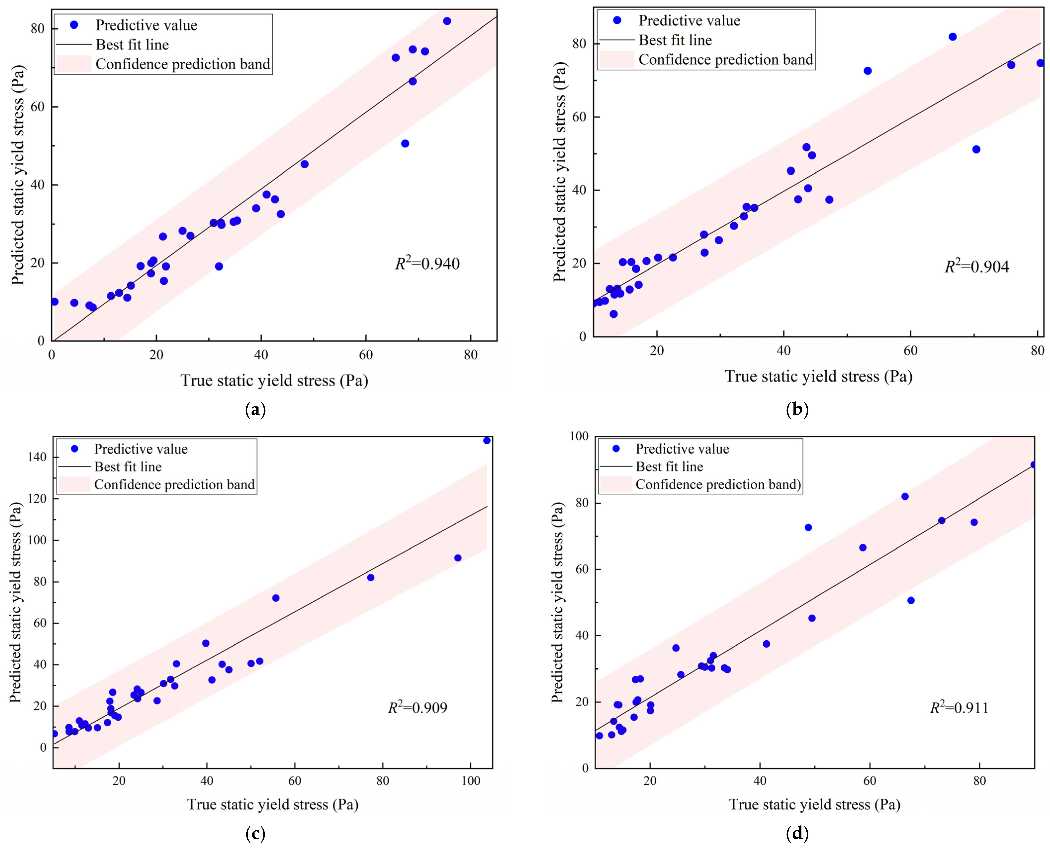
The validation diagrams for the static yield stress and dynamic yield stress prediction models are shown in Figure 7 and Figure 8. The XGBoost model performs better in predicting static and dynamic yield stress. By combining the performance of algorithms in predicting static yield stress with that of dynamic yield stress, the XGBoost model achieves the best prediction performance.
Figure 9 evaluates four machine learning models (XGBoost, ADBT, GBDT, RF) using four metrics for static (a) and dynamic (b) yield stress prediction. R2 shows that XGBoost achieves the highest values for both static (0.938) and dynamic (0.935) predictions, explaining >93% of data variability. It can be seen in MAE that ADBT shows the lowest MAE in static prediction (4.239), while XGBoost outperforms ADBT in dynamic prediction (3.115 > 2.962). RMSE shows that XGBoost attains the minimal RMSE in dynamic prediction (4.334) and static prediction (5.623). EVS shows that XGBoost peaks in both categories (static 0.94, dynamic 0.939), confirming robust interpretability for mixed design variations.
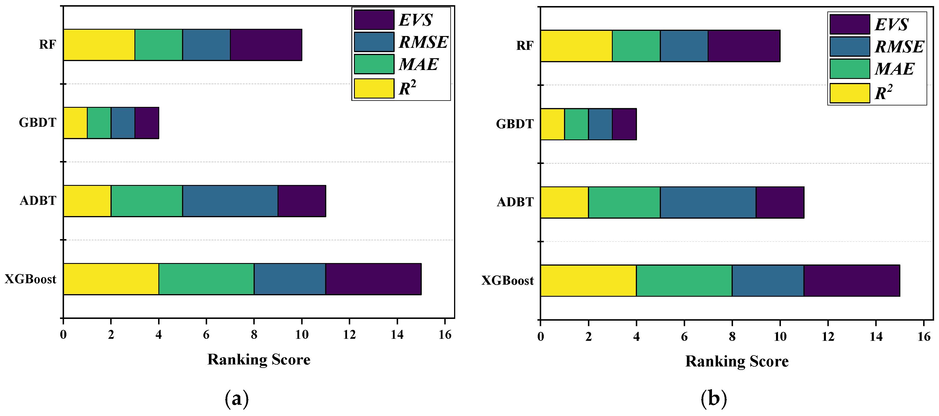
To further compare the performance of the four models mentioned above, each is scored based on the results of four indicators. Figure 10 summarizes the scores of models in a stacked graph format. It is shown that XGBoost has the highest score ranking and best performance for both the static and dynamic yield stress prediction models.

4. Results and Discussions

4.1. Effect of a Single Feature on the Yield Stress

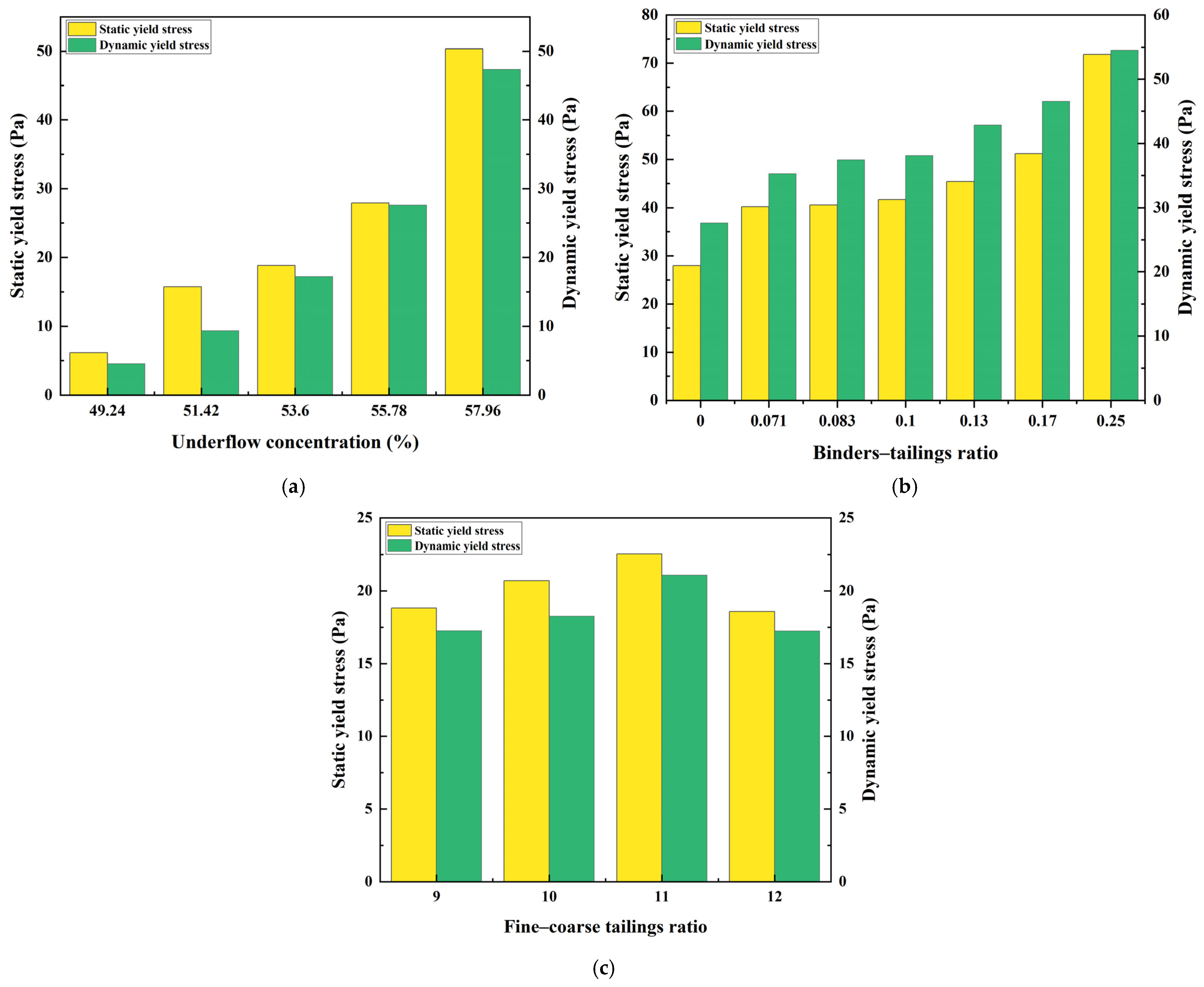
The effect of a single feature on the yield stress of the filling slurry is shown in Figure 11. It can be seen that there is a positive correlation between underflow concentration and slurry yield stress, which means that, the higher the underflow concentration, the greater the slurry static yield stress and dynamic yield stress. Notably, as the underflow concentration increased from 55.78% to 57.96%, the static yield stress increased by 80%, and the dynamic yield stress increased by 72%, indicating that the underflow concentration has a significant effect on the slurry yield stress.
Similarly, the binder-to-tailings ratio exhibited a positive correlation with yield stress (Figure 11b). Both static and dynamic yield stress increased with higher binder content, highlighting its strong contribution to rheological behavior.
In contrast, the fine-to-coarse ratio exerted only a minor influence (Figure 11c). Variations in this parameter resulted in yield stress differences of less than 4 Pa, indicating that its effect was comparatively negligible.

4.2. Effect of Feature Coupling on the Yield Stress

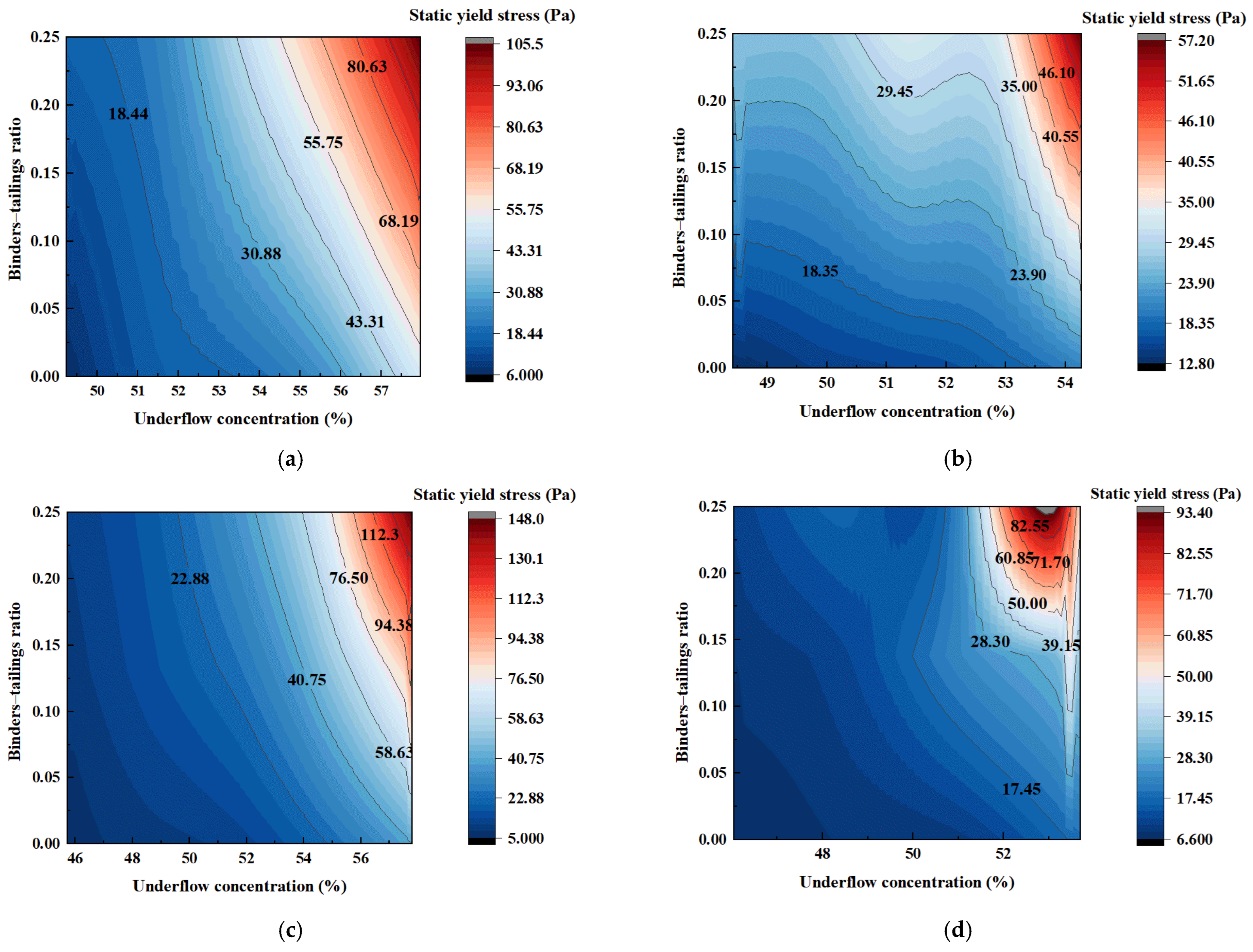
The underflow concentration and binders–tailings ratio significantly impact the rheological properties of the filling slurry. The interaction of these characteristics is shown in Figure 12. Under low underflow concentration, the contour curvature is higher for the filling slurry with a fine–coarse tailings ratio of 9:1, and the interaction between the tailings and the binders has a substantial effect on the static yield stress. At a high underflow concentration, the contour line of static yield stress is close to a straight line, suggesting that there is no strong interaction between the two parameters of binders–tailings ratio and underflow concentration. The interplay between underflow concentration and binders–tailings ratio significantly affects the static yield stress with a fine–coarse tailings ratio of 10:1; as the underflow concentration falls below 53%, the curvature of the static yield stress contour changes significantly. The interaction between the two factors of underflow concentration and binders–tailings ratio has a considerable influence on the static yield stress with a fine–coarse tailings ratio of 11:1. In the case of a fine–coarse tailings ratio of 12:1, the curvature of the static yield stress contour drastically alters as the underflow concentration exceeds 51%, and the interaction between the underflow concentration and the binders–tailings ratio has a considerable effect on the static yield stress.
Figure 13 shows the impact of the fine–coarse tailings ratio and binders–tailings ratio on the dynamic yield stress of filling slurry. It can be seen that the binders–tailings ratio has a more significant influence on the dynamic yield stress value at a low underflow concentration, and the binders–tailings ratio has less effect at a high underflow concentration, revealing that the interaction with the two features is weak. With a fine–coarse tailings ratio of 10:1, the influence of the binders–tailings ratio on the dynamic yield stress is minor for slurry at a low underflow concentration. The effect of the binders–tailings ratio on the dynamic yield stress is greater at a high underflow concentration, suggesting that the interaction between the binders–tailings ratio and the underflow concentration is stronger. As the fine–coarse tailings ratio is 11:1, the effect of the binders–tailings ratio on the dynamic yield stress is negligible at a low underflow concentration, and there exists a strong interaction between the underflow concentration and the binders–tailings ratio at a high underflow concentration. With a fine–coarse tailings ratio of 12:1, the effect of the binders–tailings ratio on the dynamic yield stress is negligible at a low underflow concentration, and the impact of the binders–tailings ratio on the dynamic yield stress is greater at a high underflow concentration. It can be seen that the underflow concentration and the binders–tailings ratio significantly impact the rheological properties of the filling slurry.

4.3. Feature Importance Analysis

The analysis in Section 3.4 demonstrates that the XGBoost algorithm predicts the static yield stress and dynamic yield stress of slurry more accurately than other algorithms. Still, it cannot directly interpret the output in detail. SHAP (Shapley additive explanation), proposed by Lundberg and Lee, is capable of quantitatively evaluating the output of a machine learning model and analyzing the role of any single feature in any sample, with the SHAP value indicating the contribution of each feature to the predicted value [44,45,46]. Assuming that the ith sample is xi, the sample has j eigenvalues, the jth feature of that sample is xij, and the SHAP value yi is calculated as
y i = y b a s e + f x i 1 + f x i 2 + + f x i j
where ybase is the model baseline, typically the mean value of the target variable for the sample. f(xij) is the SHAP value of xij, which represents the contribution of the jth feature to the predicted value yi. As f(xij) > 0 indicates that the feature plays a positive role, f(xij) < 0 means that the feature plays a negative role (meaning that the feature lowers the predicted value).
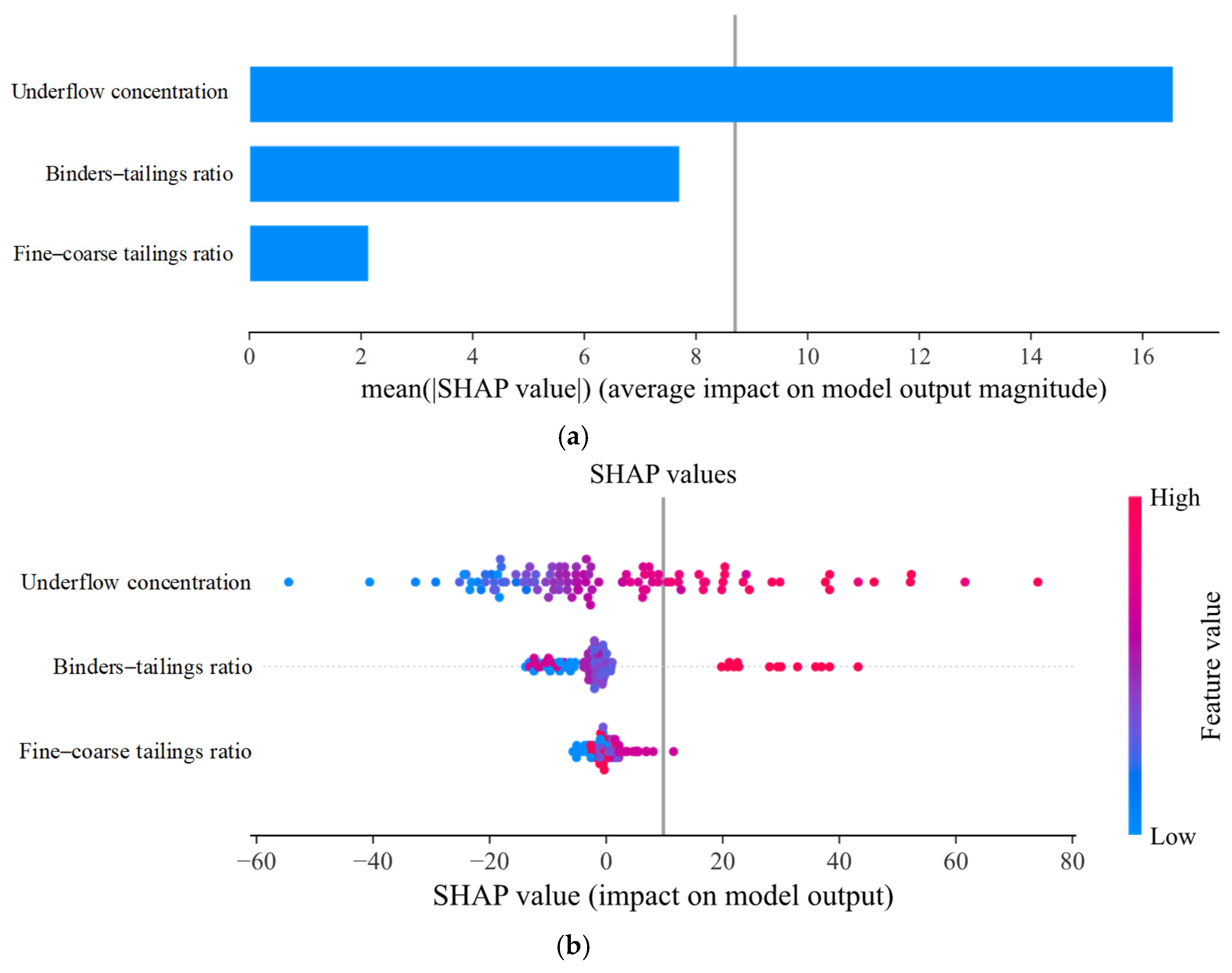
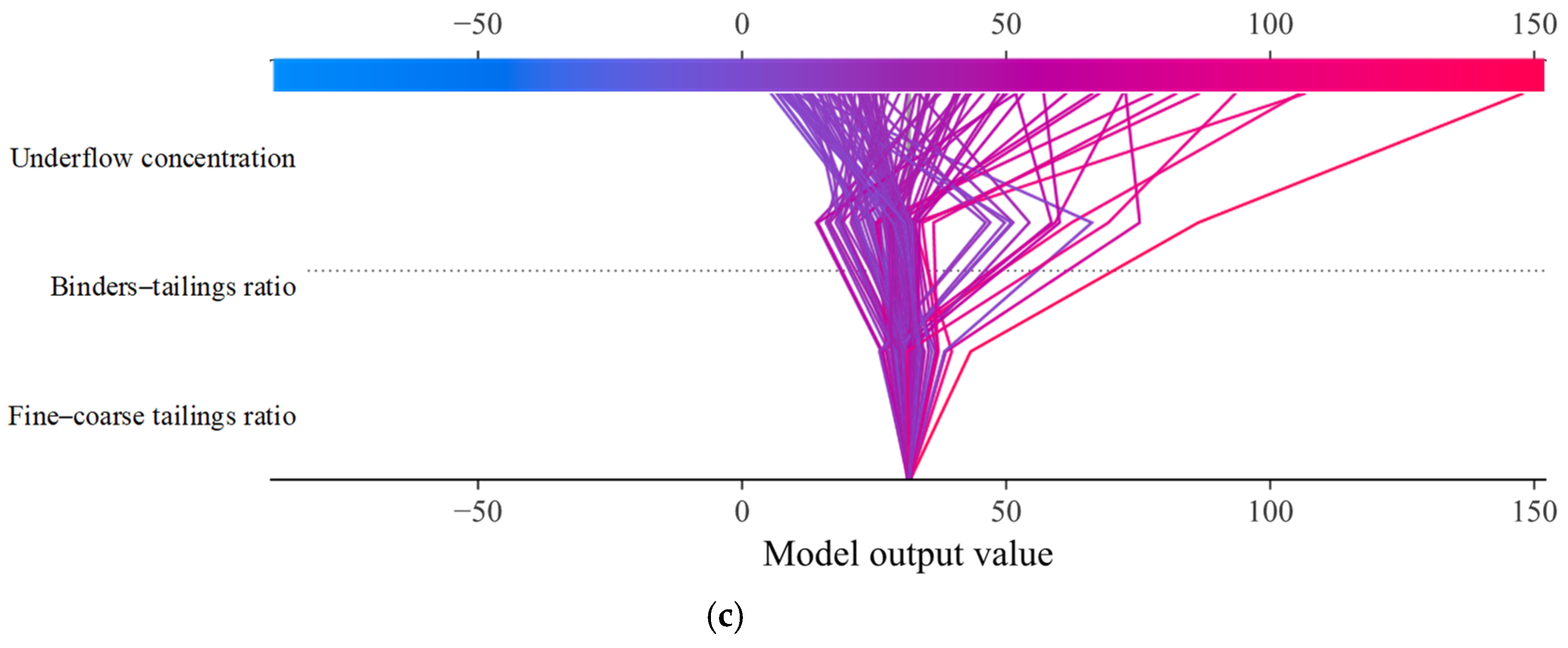
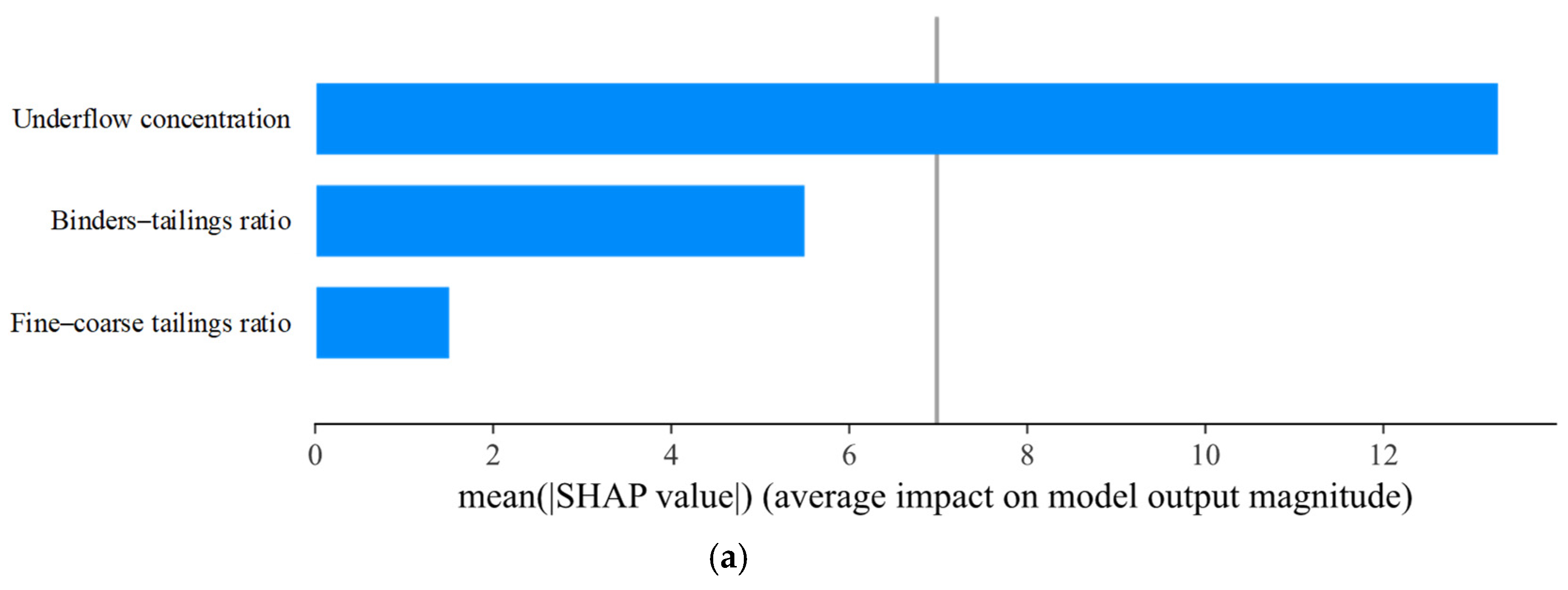
Figure 14 shows the SHAP analysis of the static yield stress prediction model, with each row representing a feature. Figure 14a shows a SHAP plot of the importance of the features. The features in the plot are ranked in order of absolute value of their influence on the model, with the features in descending order of importance being underflow concentration, binders–tailings ratio, and fine–coarse tailings ratio, with the underflow concentration being much more important than the other two features. Figure 14b is a scatter plot of the feature density of the static yield stress prediction model; the horizontal coordinates represent the corresponding SHAP values of the features, any point in the plot is a sample in the dataset, red samples represent larger feature values, and blue samples represent smaller feature values. A feature that plays a positive role in static yield stress prediction with SHAP values greater than zero with a high red point is underflow concentration; compared to the two features of binders–tailings ratio and fine–coarse tailings ratio, the underflow concentration slurry sample is more dispersed, and the underflow concentration has a more significant effect. The binders–tailings ratio is more critical for static yield stress prediction than the fine–coarse particle ratio, which contributes less to static yield stress prediction. Figure 14c is the SHAP decision plot for the static yield stress prediction model, with the x-axis showing the model output and the y-axis showing SHAP values. Each fold represents a sample resulting from a cumulative eigenvalue process. Figure 14c shows the same performance as Figure 14a,b, with the underflow concentration of the samples being more critical than the binders–tailings ratio and fine–coarse tailings ratio. The SHAP values increase significantly with underflow concentration, indicating that underflow concentration makes the most significant contribution to predicted values.
The SHAP method can also interpret the output of the dynamic yield stress prediction model. Figure 15 depicts the SHAP analysis of the dynamic yield stress model. Figure 15a shows the feature importance of dynamic yield stress, similar to the static yield stress prediction model, with the underflow concentration being most important, with an absolute value of average SHAP greater than 12, followed by the binders–tailings ratio and fine–coarse tailings ratio. Figure 15b illustrates the scatter plot for the feature density of the dynamic yield stress prediction model. The underflow concentration is critical to the model, and the SHAP values of the high underflow concentration score red points are greater than 0, indicating that underflow concentration positively affects the predicted values. In contrast, the sample distributions of the binders–tailings ratio and fine–coarse tailings ratio are mainly distributed at SHAP = 0, indicating that these two features have a minor effect on most samples. Figure 15c depicts the SHAP decision diagram for the dynamic yield stress prediction model, which yields the same results as Figure 15a,b, with the fold line significantly increased in this part of the underflow concentration. The above indicates that, for both the static and dynamic yield stress prediction models, the underflow concentration contributes most significantly to the predicted values, followed by the binders–tailings ratio and fine–coarse tailings ratio.

5. Conclusions

Cemented filling technology provides an effective approach to managing tailings and stabilizing goafs, with slurry rheology serving as a key determinant of flowability and filling body strength. In this study, static and dynamic yield stress were identified as critical parameters for evaluating slurry performance, and a predictive framework was developed using the extreme gradient boosting (XGBoost) algorithm.
A total of 140 experimental samples were used to train and validate the model (105 training, 35 testing). Three input features—underflow concentration, binder-to-tailings ratio, and fine-to-coarse ratio—were selected as predictors. Model performance was benchmarked against ADBT, GBDT, and RF algorithms using four evaluation metrics (R2, MAE, RMSE, EVS). The results demonstrated that XGBoost consistently outperformed the other models in accuracy and robustness.
The SHAP method was further applied to interpret the model predictions. Feature importance analysis revealed that the underflow concentration contributed most to yield stress predictions, followed by the binder-to-tailings ratio, with the fine-to-coarse ratio exerting the least influence.
Limitations and future work:
This study considered only three influencing factors. Additional material properties, such as particle size distribution and gradation, are known to affect slurry rheology and should be incorporated to further improve prediction accuracy. Future research will also explore hybrid machine learning models (e.g., WOA-XGBoost, GWO-XGBoost, BO-XGBoost) to leverage their complementary strengths and enhance generalization across different tailings types.
Practical implications:
By integrating machine learning into slurry design, the proposed framework simplifies the prediction of rheological parameters, reduces experimental costs, and offers a powerful tool for optimizing cemented filling technology in engineering practice.

Supplementary Materials

The following supporting information can be downloaded at: https://www.mdpi.com/article/10.3390/min15090931/s1, Figure S1. The flow curve of the filling slurry with a fine-to-coarse tailings ratio of 9:1. Figure S2. The flow curve of the filling slurry with a fine-to-coarse tailings ratio of 10:1. Figure S3. The flow curve of the filling slurry with a fine-to-coarse tailings ratio of 11:1. Table S1. Results of rheological experiment on Paste.

Author Contributions

Methodology, X.L. and X.C.; Software, R.T. and Z.X.; Validation, R.T. and X.C.; Formal analysis, R.T.; Investigation, Z.X. and H.D.; Writing—original draft, X.L.; Writing—review & editing, K.Q. and H.D.; Visualization, X.L.; Supervision, K.Q.; Project administration, K.Q.; Funding acquisition, Z.X. and H.D. All authors have read and agreed to the published version of the manuscript.

Funding

This work received financial support from Yunnan Fundamental Research Projects (No. 202501CF070049, No. 202501CF070050).

Data Availability Statement

All data generated or analyzed during this study are included in this article and its Supplementary Materials.

Conflicts of Interest

Author Xue Li was employed by the company Kunming Metallurgical Research Institute Co., Ltd. The remaining authors declare that the research was conducted in the absence of any commercial or financial relationships that could be construed as a potential conflict of interest.

References

  1. Cai, M.F.; Xue, D.L.; Ren, F.H. Current status and development strategy of metal mines. Chin. J. Eng. 2019, 41, 417–426. [Google Scholar] [CrossRef]
  2. Nguyen, Q.D.; Boger, D.V. Application of rheology to solving tailings disposal problems. Int. J. Miner. Process. 1998, 54, 217–233. [Google Scholar] [CrossRef]
  3. Wang, C.; Harbottle, D.; Liu, Q.; Xu, Z. Current state of fine mineral tailings treatment: A critical review on theory and practice. Miner. Eng. 2014, 58, 113–131. [Google Scholar] [CrossRef]
  4. Hui, Y.H.; Cai, L.B.; Liu, W.; Qin, W.Q.; Jiao, F.; Yang, C.R. Current status and development of comprehensive utilization of waste rock in metal mines in China. Chin. J. Nonferrous Met. 2021, 31, 1649–1660. [Google Scholar]
  5. Santamarina, J.C.; Torres-Cruz, L.A.; Bachus, R.C. Why did the tailings dam at Brumadinho fail? Eng. Geol. 2021, 294, 106339. [Google Scholar] [CrossRef]
  6. Ministry of Industry and Information Technology (MIIT). Management Measures for the Prevention and Control of Environmental Pollution by Tailings; MIIT: Beijing, China, 2022. Available online: https://www.gov.cn/gongbao/content/2022/content_5697980.htm (accessed on 6 April 2022).
  7. Landriault, D.; Verburg, R.; Cincilla, W.; Welch, D. Paste technology for underground backfill and surface tailings disposal applications. In Short Course Notes; Technical Workshop œ April; Canadian Institute of Mining and Metallurgy: Westmount, QC, USA, 1997; p. 121. [Google Scholar]
  8. Chen, H.J.; Liu, Q.J. Harms and Resource-like Treatment of the Solid Wastes from Metal Mines. Met. Mine 2009, 4, 154–156+167. [Google Scholar] [CrossRef]
  9. Yin, S.; Shao, Y.; Wu, A.; Wang, H.; Liu, X.; Wang, Y. A systematic review of paste technology in metal mines for cleaner production in China. J. Clean. Prod. 2020, 247, 119590. [Google Scholar] [CrossRef]
  10. Yang, K.; Zhao, X.; Wei, Z.; Zhang, J. Development overview of paste backfill technology in China’s coal mines: A review. Environ. Sci. Pollut. Res. 2021, 28, 67957–67969. [Google Scholar] [CrossRef]
  11. Wu, A.X.; Yang, Y.; Cheng, H.Y.; Chen, S.M.; Han, Y. Status and prospects of paste technology in China. Chin. J. Eng. 2018, 40, 517–525. [Google Scholar] [CrossRef]
  12. Zhou, Z.; Liu, J.; Zhou, Q.; Wu, A.; Wang, H. A New High Charge Density Superplasticizer Regulates the Rheological Properties of Tailings Slurry and Cemented Paste Backfill Materials. Min. Metall. Explor. 2022, 39, 749–759. [Google Scholar] [CrossRef]
  13. Yang, L.H.; Wang, H.J.; Wu, A.X.; Gao, W.H. Status and Development Tendency of the Full-tailings Paste Mixing Technology. Met. Mine 2016, 7, 34–41. [Google Scholar]
  14. Wu, A.X.; Li, H.; Cheng, H.Y.; Wang, Y.M.; Li, C.P.; Ruan, Z.E. Status and prospects of researches on rheology of paste backfill using unclassified tailings (Part 1): Concepts, characteristics and models. Chin. J. Eng. 2020, 42, 803–813. [Google Scholar] [CrossRef]
  15. Wang, S.; Song, X.; Wei, M.; Liu, W.; Wang, X.; Ke, Y.; Tao, T.; Liu, H. Flow Characteristics of Fresh Cemented Paste Backfill Containing Flocculant under Variable Shear Rate Based on Water Migration. Min. Metall. Explor. 2022, 39, 1189–1203. [Google Scholar] [CrossRef]
  16. Hu, C.F.; Li, C.P.; Yan, B.H.; Chen, G.Z. Effect of water reducing agent on rheological property of fine-grained tailings paste. Chin. J. Nonferrous Met. 2022, 32, 2458–2468. [Google Scholar] [CrossRef]
  17. Chen, F.B.; Su, R.; Yang, L.H.; Jiao, H.Z.; Wu, A.X.; Yin, S.H.; Wang, H.J.; Gao, Y.; Kou, Y.P.; Wang, Z.J. Effect of mixing speed on rheological properties of cemented paste backfill. Chin. J. Nonferrous Met. 2022, 32, 3541–3552. [Google Scholar] [CrossRef]
  18. Zhang, X.X.; Qiao, D.P. Rheological properties and yield stress prediction model of waste rock-tailings high concentration slurry. J. Saf. Environ. 2015, 15, 278–283. [Google Scholar]
  19. Zhang, Q.L.; Liu, W.J.; Wang, X.M.; Chen, Q.S. Optimal prediction model of backfill paste rheological parameters. J. Cent. South Univ. Sci. Technol. 2018, 49, 124–130. [Google Scholar]
  20. Yan, B.H.; Li, C.P.; Wang, S.Y.; Hou, H.Z. Measurement of Rheological Parameters for the Whole-tailing Paste and Optimization of the Rheological Models. Met. Mine 2017, 12, 44–48. [Google Scholar]
  21. Liu, X.H.; Wu, A.X.; Wang, H.J.; Wang, Y.M. Influence mechanism and calculation model of CPB rheological parameters. Chin. J. Eng. 2017, 39, 190–195. [Google Scholar]
  22. Qi, C.C.; Fourie, A. Cemented paste backfill for mineral tailings management: Review and future perspectives. Miner. Eng. 2019, 144, 106025. [Google Scholar] [CrossRef]
  23. Sun, Y.; Li, G.; Zhang, J.; Sun, J.; Xu, J. Development of an Ensemble Intelligent Model for Assessing the Strength of Cemented Paste Backfill. Adv. Civ. Eng. 2020, 2020, 1–6. [Google Scholar] [CrossRef]
  24. Du, K.; Liu, M.; Zhou, J.; Khandelwal, M. Investigating the Slurry Fluidity and Strength Characteristics of Cemented Backfill and Strength Prediction Models by Developing Hybrid GA-SVR and PSO-SVR, Mining. Metall. Explor. 2022, 39, 433–452. [Google Scholar] [CrossRef]
  25. Farooq, F.; Ahmed, W.; Akbar, A.; Aslam, F.; Alyousef, R. Predictive modeling for sustainable high-performance concrete from industrial wastes: A comparison and optimization of models using ensemble learners. J. Clean. Prod. 2021, 292, 126032. [Google Scholar] [CrossRef]
  26. Ramzi, M.; Kashaninejad, M.; Salehi, F.; Sadeghi Mahoonak, A.R.; Ali Razavi, S.M. Modeling of rheological behavior of honey using genetic algorithm–artificial neural network and adaptive neuro-fuzzy inference system. Food Biosci. 2015, 9, 60–67. [Google Scholar] [CrossRef]
  27. Ghaffarkhah, A.; Bazzi, A.; Dijvejin, Z.A.; Talebkeikhah, M.; Moraveji, M.K.; Agin, F. Experimental and numerical analysis of rheological characterization of hybrid nano-lubricants containing COOH-Functionalized MWCNTs and oxide nanoparticles. Int. Commun. Heat Mass Transf. 2019, 101, 103–115. [Google Scholar] [CrossRef]
  28. Shahsavar, A.; Jamei, M.; Karbasi, M. Experimental evaluation and development of predictive models for rheological behavior of aqueous Fe3O4 ferrofluid in the presence of an external magnetic field by introducing a novel grid optimization based-Kernel ridge regression supported by sensitivity analysis. Powder Technol. 2021, 393, 1–11. [Google Scholar] [CrossRef]
  29. Asadi, A.; Alarifi, I.M.; Nguyen, H.M.; Moayedi, H. Feasibility of least-square support vector machine in predicting the effects of shear rate on the rheological properties and pumping power of MWCNT–MgO/oil hybrid nanofluid based on experimental data. J. Therm. Anal. Calorim. 2021, 143, 1439–1454. [Google Scholar] [CrossRef]
  30. Gomaa, E.; Han, T.; ElGawady, M.; Huang, J.; Kumar, A. Machine learning to predict properties of fresh and hardened alkali-activated concrete. Cem. Concr. Compos. 2021, 115, 103863. [Google Scholar] [CrossRef]
  31. Nehdi, M.; Al Martini, S. Estimating time and temperature dependent yield stress of cement paste using oscillatory rheology and genetic algorithms. Cem. Concr. Res. 2009, 39, 1007–1016. [Google Scholar] [CrossRef]
  32. Nguyen, T.-D.; Tran, T.-H.; Hoang, N.-D. Prediction of interface yield stress and plastic viscosity of fresh concrete using a hybrid machine learning approach. Adv. Eng. Inform. 2020, 44, 101057. [Google Scholar] [CrossRef]
  33. Chen, T.Q.; Guestrin, C. Xgboost: A scalable tree boosting system. In Proceedings of the 22nd ACM SIGKDD International Conference on Knowledge Discovery and Data Mining, San Francisco, CA, USA, 13–17 August 2016; pp. 785–794. [Google Scholar] [CrossRef]
  34. Shehadeh, A.; Alshboul, O.; Al Mamlook, R.E.; Hamedat, O. Machine learning models for predicting the residual value of heavy construction equipment: An evaluation of modified decision tree, LightGBM, and XGBoost regression. Autom. Constr. 2021, 129, 103827. [Google Scholar] [CrossRef]
  35. Nguyen, N.-H.; Abellán-García, J.; Lee, S.; Garcia-Castano, E.; Vo, T.P. Efficient estimating compressive strength of ultra-high performance concrete using XGBoost model. J. Build. Eng. 2022, 52, 104302. [Google Scholar] [CrossRef]
  36. Li, C.; Yan, B.; Wang, S.; Hou, H.; Chen, G. Variability behavior of yield stress for unclassified tailings pasted under measurement time–velocity double factors. Chin. J. Eng. 2020, 42, 1308–1317. [Google Scholar] [CrossRef]
  37. Huang, Z.; Li, C.; Li, X.; Ruan, Z.; Wang, S. Volume Concentration Effect on Rheology of Filling Slurry with Different Material Ratios. Mater. Rep. 2023, 37, 102–110. [Google Scholar]
  38. Jiao, D.; Shi, C.; Yuan, Q. Time-dependent rheological behavior of cementitious paste under continuous shear mixing. Constr. Build. Mater. 2019, 226, 591–600. [Google Scholar] [CrossRef]
  39. Mahaut, F.; Mokéddem, S.; Chateau, X.; Roussel, N.; Ovarlez, G. Effect of coarse particle volume fraction on the yield stress and thixotropy of cementitious materials. Cem. Concr. Res. 2008, 38, 1276–1285. [Google Scholar] [CrossRef]
  40. Li, H.; Cao, Y.; Li, S.; Zhao, J.; Sun, Y. XGBoost model and its application to personal credit evaluation. IEEE Intell. Syst. 2020, 35, 52–61. [Google Scholar] [CrossRef]
  41. Qi, C.; Fourie, A.; Chen, Q.; Zhang, Q. A strength prediction model using artificial intelligence for recycling waste tailings as cemented paste backfill. J. Clean. Prod. 2018, 183, 566–578. [Google Scholar] [CrossRef]
  42. Cao, J.; Gao, J.; Nikafshan Rad, H.; Mohammed, A.S.; Hasanipanah, M.; Zhou, J. A novel systematic and evolved approach based on XGBoost-firefly algorithm to predict Young’s modulus and unconfined compressive strength of rock. Eng. Comput. 2021, 38 (Suppl. S5), 3829–3845. [Google Scholar] [CrossRef]
  43. Duan, J.; Asteris, P.G.; Nguyen, H.; Bui, X.-N.; Moayedi, H. A novel artificial intelligence technique to predict compressive strength of recycled aggregate concrete using ICA-XGBoost model. Eng. Comput. 2021, 37, 3329–3346. [Google Scholar] [CrossRef]
  44. Lundberg, S.M.; Lee, S.-I. A Unified Approach to Interpreting Model Predictions. arXiv 2017, arXiv:1705.07874. [Google Scholar] [CrossRef]
  45. Parsa, A.B.; Movahedi, A.; Taghipour, H.; Derrible, S.; Mohammadian, A.K. Toward safer highways, application of XGBoost and SHAP for real-time accident detection and feature analysis. Accid. Anal. Prev. 2020, 136, 105405. [Google Scholar] [CrossRef]
  46. Chang, I.; Park, H.; Hong, E.; Lee, J.; Kwon, N. Predicting effects of built environment on fatal pedestrian accidents at location-specific level: Application of XGBoost and SHAP. Accid. Anal. Prev. 2022, 166, 106545. [Google Scholar] [CrossRef]
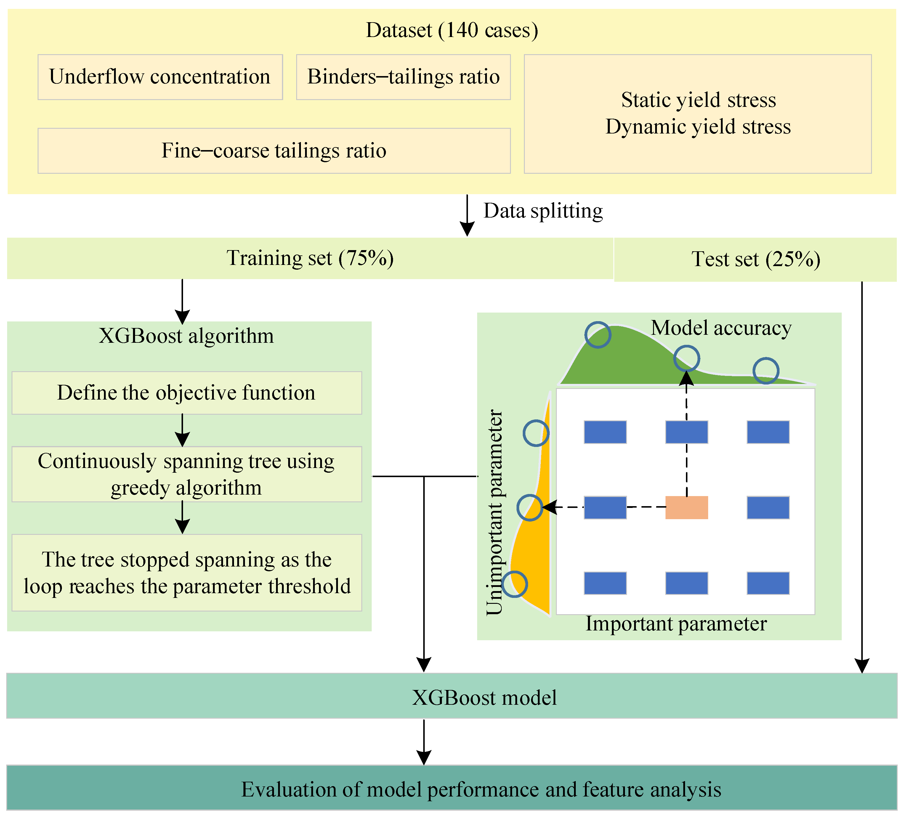
Figure 1. Framework of the XGBoost method for determining the yield stress of slurry.
Minerals 15 00931 g001
Figure 2. Particle size distribution of the fine tailings and the binder. (a) Fine tailings; (b) binders.
Minerals 15 00931 g002
Figure 3. Schematic of the rheological testing program.
Minerals 15 00931 g003
Figure 4. Flow curves of slurry at a fine-to-coarse ratio of 12:1. (a) Underflow concentration 46.04%; (b) underflow concentration 48.59%; (c) underflow concentration 51.14%; (d) underflow concentration 53.69%; (e) underflow concentration 56.24%.
Minerals 15 00931 g004
Figure 5. Contour graphs of features versus yield stress.
Minerals 15 00931 g005
Figure 6. Iteration process for static and dynamic yield stress models. (a) Static yield stress prediction model; (b) dynamic yield stress prediction model.
Minerals 15 00931 g006
Figure 7. Validation diagram of static yield stress prediction model. (a) XGBoost; (b) ADBT; (c) GBDT; (d) RF.
Minerals 15 00931 g007
Figure 8. Validation diagram of dynamic yield stress prediction model. (a) XGBoost; (b) ADBT; (c) GBDT; (d) RF.
Minerals 15 00931 g008
Figure 9. Results for each type of model in the test set. (a) Static yield stress prediction model; (b) dynamic yield stress prediction model.
Minerals 15 00931 g009
Figure 10. Intuitive display of the ranking scores of the four models. (a) Static yield stress prediction model; (b) dynamic yield stress prediction model.
Minerals 15 00931 g010
Figure 11. Effect of a single feature on the filling slurry yield Stress. (a) Underflow concentration; (b) binders–tailings ratio; (c) fine–coarse tailings ratio.
Minerals 15 00931 g011
Figure 12. Effect of multi-feature coupling on the static yield stress. (a) Fine-coarse tailings ratio = 9:1; (b) Fine-coarse tailings ratio = 10:1; (c) Fine-coarse tailings ratio = 11:1; (d) Fine-coarse tailings ratio = 12:1.
Minerals 15 00931 g012
Figure 13. Effect of multi-feature coupling on dynamic yield stress. (a) Fine–coarse tailings ratio = 9:1; (b) fine–coarse tailings ratio = 10:1; (c) fine–coarse tailings ratio = 11:1; (d) fine–coarse tailings ratio = 12:1.
Minerals 15 00931 g013
Figure 14. SHAP analysis diagram for the static yield stress prediction model. (a) Feature importance diagram for the static yield stress prediction model; (b) scatter plot for the feature density of the static yield stress prediction model; (c) decision diagram for the static yield stress prediction model.
Minerals 15 00931 g014aMinerals 15 00931 g014b
Figure 15. SHAP analysis diagram for the dynamic yield stress prediction model. (a) Feature importance diagram for the dynamic yield stress prediction model; (b) scatter plot for the feature density of the dynamic yield stress prediction model; (c) decision diagram for the dynamic yield stress prediction model.
Minerals 15 00931 g015aMinerals 15 00931 g015b
Table 1. Particle size distribution of the coarse tailings.
Particle Size150–220 μm220–400 μm400–500 μm500–630 μm630–800 μm800–1000 μm
Percentage20.61%20.52%8.89%13.86%28.18%7.85%
Table 2. Chemical composition of the tailings and binder.
MaterialOxide (wt%)
SiO2MgOFe2O3Al2O3CaOP2O5K2OSO3Others
Tailing41.2515.0012.6012.0310.023.183.110.821.99
Binders29.765.361.4315.9737.95-0.507.21.20
Table 3. Experimental influencing factors and level settings.
Influence FactorsExperimental Level
Fine–coarse tailings ratio9:1, 10:1, 11:1, 12:1
Binders–tailings ratio0, 1:14, 1:12, 1:10, 1:8, 1:6, 1:4
Underflow concentrationFine–coarse tailings ratio 9:149.24%, 51.42%, 53.6%, 55.78%, 57.96%
Fine–coarse tailings ratio 10:148.43%, 49.89%, 51.35%, 52.81%, 54.27%
Fine–coarse tailings ratio 11:145.72%, 48.74%, 51.76%, 54.78%, 57.8%
Fine–coarse tailings ratio 12:146.04%, 48.59%, 51.14%, 53.69%, 56.24%
Table 4. Model performance evaluation indicators.
IndicatorDescriptionEquation
R2Describes regression model variance score, with a range of from (0, 1], with larger values indicating higher accuracy of the prediction model R 2 = 1 S S E S S T
MAEEvaluates how close the predictions are to the true dataset; the smaller the value, the better the fit M A E = i = 1 n Y S p i Y S t i n
RMSEExplains distribution of forecast errors, with smaller values of RMSE indicating less variation in forecast distribution R M S E = i = 1 n Y S p i Y S t i 2 n
EVSDefines a model variance score in the range of (0, 1], with larger values being more effective E V S = 1 n S S E M E n S S T
Notes: YSpi is the predicted yield stress value, YSti is the true yield stress value, SSE is the sum of squared errors, SST is the sum of total squares, and ME is the mean residual.
Table 5. Optimized hyperparameter settings.
Parameter ClassificationParameterInitial SettingStatic Yield Stress
Model Results
Dynamic Yield Stress Model Results
Tree boosterEta0.05–0.30.150.16
Min_child_weight111
Max_depth[3, 10]45
Gamma[0, 0.2]0.10.1
Subsample[0.5, 0.9]0.80.72
Colsample_bytree[0, 1]0.760.78
Alpha100
Lambda122
Learning TaskObjectiveLinearRegressionLinearRegressionLinearRegression
Eval_metricRMSERMSERMSE
Command lineNum_round500400300
Disclaimer/Publisher’s Note: The statements, opinions and data contained in all publications are solely those of the individual author(s) and contributor(s) and not of MDPI and/or the editor(s). MDPI and/or the editor(s) disclaim responsibility for any injury to people or property resulting from any ideas, methods, instructions or products referred to in the content.