Article

Hyperspectral Lithological Classification of 81 Rock Types Using Deep Ensemble Learning Algorithms

by
Shanjuan Xie
1,*,
Yichun Qiu
2,
Shixian Cao
1 and
Wenyuan Wu
1,3
1
School of Information Science and Technology, Hangzhou Normal University, Hangzhou 311121, China
2
Kharkiv College, Hangzhou Normal University, Hangzhou 311121, China
3
Zhejiang Provincial Key Laboratory of Urban Wetlands and Regional Change, Hangzhou Normal University, Hangzhou 311121, China
*
Author to whom correspondence should be addressed.
Minerals 2025, 15(8), 844; https://doi.org/10.3390/min15080844
Submission received: 5 July 2025 / Revised: 1 August 2025 / Accepted: 6 August 2025 / Published: 8 August 2025
(This article belongs to the Section Mineral Exploration Methods and Applications)

Abstract

To address overfitting due to limited sample size, and the challenges posed by “Spectral Homogeneity with Material Heterogeneity (SHMH)” and “Material Consistency with Spectral Divergence (MCSD)”—which arise from subtle spectral differences and limited classification accuracy—this study proposes a deep integration model that combines the Adaptive Boosting (AdaBoost) algorithm with a convolutional recurrent neural network (CRNN). The model adopts a dual-branch architecture integrating a 2D-CNN and gated recurrent unit to effectively fuse spatial and spectral features of rock samples, while the integration of the AdaBoost algorithm optimizes performance by enhancing system stability and generalization capability. The experiment used a hyperspectral dataset containing 81 rock samples (46 igneous rocks and 35 metamorphic rocks) and evaluated model performance through five-fold cross-validation. The results showed that the proposed 2D-CRNN-AdaBoost model achieved 92.55% overall accuracy, which was significantly better than that of other comparative models, demonstrating the effectiveness of multimodal feature fusion and ensemble learning strategy.

1. Introduction

Rocks are fundamental components of the Earth’s surface and are essential for accurate classification in fields such as geotechnical engineering, mineralogy, petrology, rock mechanics, and mineral resource exploration [1,2,3].
In geological research, rock classification and nomenclature systems facilitate the differentiation of rock types and their spatial distribution across distinct regions, thereby enhancing exploration efficiency. For example, Li et al. [4] demonstrated the critical role of lithological classification in guiding geological surveys and mineral prospecting. By identifying the types of Yanshanian granites, their research revealed potential genetic linkages to Mo-polymetallic mineralization, underscoring the practical value of systematic rock categorization in mineral resource targeting. Similarly, analyzing the microstructural characteristics of melt inclusions in anatectic metamorphic rocks necessitates precise rock classification and petrographic identification using traditional methodologies [5].
Classification methods predominantly rely on field-based macroscopic observations and laboratory microscopic identification. For example, the approach proposed by Xu et al. (2014) [6] involves field collection of rock spectra coupled with EO-1 Hyperion data matching to identify lithological types. However, such conventional methodologies suffer from limitations including low efficiency, strong subjectivity, and limited adaptability to complex geological environments. In recent years, hyperspectral imaging technology, leveraging its nanometer-scale spectral resolution (λ/100) and broad spectral coverage, has enabled the simultaneous resolution of microscale compositional variations and macroscale structural features in rocks, providing a strong technical foundation for intelligent lithological classification [7]. This advancement has been increasingly applied to geological mapping [8] and mineral resource exploration [9].
The development of hyperspectral rock classification methodologies has progressed through two pivotal phases. The first, centered on traditional machine learning, primarily employed algorithms such as spectral angle mapper [10], random forest [11,12], K-means clustering [13], and support vector machine [14]. For example, Tessier et al. [15] successfully classified desiccated rock mixtures by integrating wavelet texture analysis with SVM, while Tripathi and Garg [16] employed principal component analysis (PCA)-based dimensionality reduction and K-means clustering to identify basalt subtypes. However, these methods faced significant limitations due to the curse of dimensionality—also known as the Hughes phenomenon [17]—inherent in hyperspectral data. While subsequent hybrid methods like Kilickaya et al. [18] integrated subspace learning with one-class classification to eliminate cascaded errors from traditional separate dimensionality reduction and classification, their insufficient spatial-spectral feature decoupling capability still limits classification performance in complex geological scenarios.
The breakthrough of convolutional neural networks (CNNs) [19] in image processing has spurred researchers to explore end-to-end feature learning frameworks for the hyperspectral classification of rocks. For example, Yang et al. [20] implemented 1D-CNNs to classify coal and rock spectral curves, while Zhang et al. [21] used the fusion strategy of 2D-CNN and 1D-CNN to capture spatial correlation [22], enabling coarse classification of airborne hyperspectral rock images. However, single-modal feature extraction remains insufficient for addressing the complexity of geological environments. Sinaice et al. [23] successfully distinguished eight igneous rock units with 96% prediction accuracy by combining hyperspectral imaging with deep learning CNN technology; however, the experiment only covered a few igneous rock samples and could not fully represent more rock types.
The comprehensive development of deep learning has promoted the formation of a space-spectrum joint learning paradigm. Hyperspectral rock imagery exhibits dual attributes [24]: spatial features reflect tectonic features (e.g., stratification and joint development), while spectral features encode mineral chemical composition information [25]. These dual properties necessitate that algorithms possess multiscale feature fusion capabilities to holistically integrate spatial context and spectral signatures for robust lithological discrimination.
The dual-stream CNN architecture developed by Dang et al. [26] achieved an accuracy of 89.2% in granite classification, demonstrating the efficacy of spatial-spectral collaborative learning. Subsequent studies further incorporated temporal modeling techniques to enhance spectral sequence analysis [27]. For example, Zhao et al. [28] developed a Long Short-Term Memory and convolutional neural network (LSTM-CNN) hybrid network, validating its effectiveness in spectral-temporal feature extraction on the airborne visible/infrared imaging spectrometer copper ore dataset (1990–2480 nm). Agrawal and Govil [29] addressed training instability in multi-layer LSTM stacks by proposing residual connections integrating 1D-CNN and LSTM modules, achieving recognition accuracies of 92% and 89% for alunite and calcite, respectively. Notably, Liu et al. [30] adopted the implementation of rock thin section mineral grain classification, which improved the overall recognition rate by approximately 4% compared with the ResNet + LSTM method (93.2%), demonstrating better engineering applicability.
However, existing approaches face three core challenges:
Inadequate dataset foundations: Existing datasets exhibit critical constraints in lithological diversity. For instance, the Okada Mineral Set [31] covers only five mineral types, while the Galdames dataset [32] expands coverage to thirteen rock types—including andesite, tourmaline breccia, and travertine breccia. Nevertheless, the persistent lack of spectral variability analysis fundamentally restricts their applicability to complex rock identification and classification scenarios.
Small-sample generalization deficit: Data scarcity induces severe overfitting and accuracy degradation, especially for metamorphic rocks. As evidenced by Li et al. [33], the ShufflNetV2 model misclassified 46 metamorphic rock samples as volcanic rocks when using deep learning to classify thin rock section images, while the overall accuracy (OA) of metamorphic rocks was the lowest (67%).
Spectral confusion: Spectral Homogeneity with Material Heterogeneity (SHMH) and Spectral Heterogeneity for Compositionally Similar Deposits (MCSD) disrupt the spectral-lithological correspondence, significantly compromising the recognition accuracy of mainstream classification models. SHMH refers to the spectral uniformity arising from the overlapping of key mineral absorption features in different lithologies. For instance, Zhang et al. [34] discovered spectral overlap in certain mineral assemblages. Barbey et al. [35] observed that the reflection curves of cordierite hornfels and granite converge in the 2200–2400 nm band due to overlapping Fe2+ absorption features. Regmi [36] confirmed that metamorphic hornfels and granite exhibit similarities in Al-OH absorption due to their shared ferromagnesian minerals.
MCSD refers to the spectral divergence observed within the same lithology caused by internal variations in mineral structure or alteration. For example, Karimzadeh and Tangestani [37] found that spectral ratio characteristics vary in chlorite-serpentinite schist due to differentiation in alteration.
In response to the above challenges, this study conducted breakthrough explorations at two levels: data foundation construction and algorithm architecture innovation. First, a laboratory-grade imaging spectrometer was used to construct a standard hyperspectral rock dataset (HSRD-1.0) encompassing 46 igneous and 35 metamorphic rock types, with a focus on spectrally ambiguous lithologies. Next, an Adaptive Boosting (AdaBoost)-enhanced convolutional recurrent neural network (2D-CRNN) ensemble framework was proposed, featuring a dual-branch architecture for dynamically fusing spatial and spectral features—effectively mitigating the issue of homospectrality. Furthermore, ablation experiments on deformable convolutional layers demonstrated that the adaptive sample weighting mechanism significantly enhanced recognition accuracy and robustness for small-sample categories, offering a systematic solution to class imbalance in hyperspectral rock image classification.

2. Hardware and Dataset

2.1. Hyperspectral Imaging System

This study adopted the HySpex SWIR-384 push-broom hyperspectral imaging system (as shown in Figure 1), which is designed with a push-broom moving platform, featuring a 16-degree field of view, 384 × 288 pixels, a spectral range of 950–2500 nm (5.45 nm resolution), and 16-bit data accuracy. It is equipped with an automatic focusing function to achieve high-precision multispectral imaging in moving scenes.

2.2. Hyperspectral Rock Standard Dataset HSRD-1.0

A total of 81 geologically representative newly exposed rock samples were selected, among which No. 1 to No. 46 were magmatic rocks, and No. 47 to No. 81 were metamorphic rocks (see Figure 2a for classification display). Magmatic rock samples are of great importance in the fields of geothermal development, metallurgical industry, and geological scientific research because of their high resistance to high temperatures and high compressive strength. Metamorphic rocks (such as gneiss and marble) are susceptible to the superposition of multi-stage metamorphism due to mineral recrystallization and structural complexity (such as foliation and banded structure), resulting in the overlapping of absorption peaks between bands (such as the similar response of epidote and amphibole at 1200–1400 nm), which poses a greater challenge to the spectral resolution of classification models. However, crustal evolution records and the development potential of new building materials highlight the necessity of high-precision identification.
During the collection of rock sample data, to eliminate sensor noise and environmental interference, the research team adopted the whiteboard calibration technique to obtain true reflectance data. Specifically, using a standard whiteboard with a reflectance close to 100% as the benchmark, the spectral reflectance calculation was performed according to Equation (1)
R = H · R w E w
where H represents the hyperspectral emissivity image (raw sensor data); R w is the pre-calibrated reflectivity of the white reference board; and E w   denotes the emissivity of the whiteboard, which is used to normalize the sensor’s emissivity measurements and derive accurate surface reflectivity.
The corrected hyperspectral pseudo-color image is shown in Figure 2b, which effectively improves the signal-to-noise ratio of the original data.
This visualization method can directly reflect the spectral absorption characteristics of different rock types, laying a foundation for subsequent mineral composition analysis. For the issue of blurred edges and shadow interference in rock sample images, the study innovatively applied a 5 × 5 erosion algorithm to morphologically process the sample edges (the processing effect comparison is shown in Figure 2c). This method effectively eliminates the effect of boundary abnormal pixels on spectral feature extraction, improving the accuracy of the classification model.
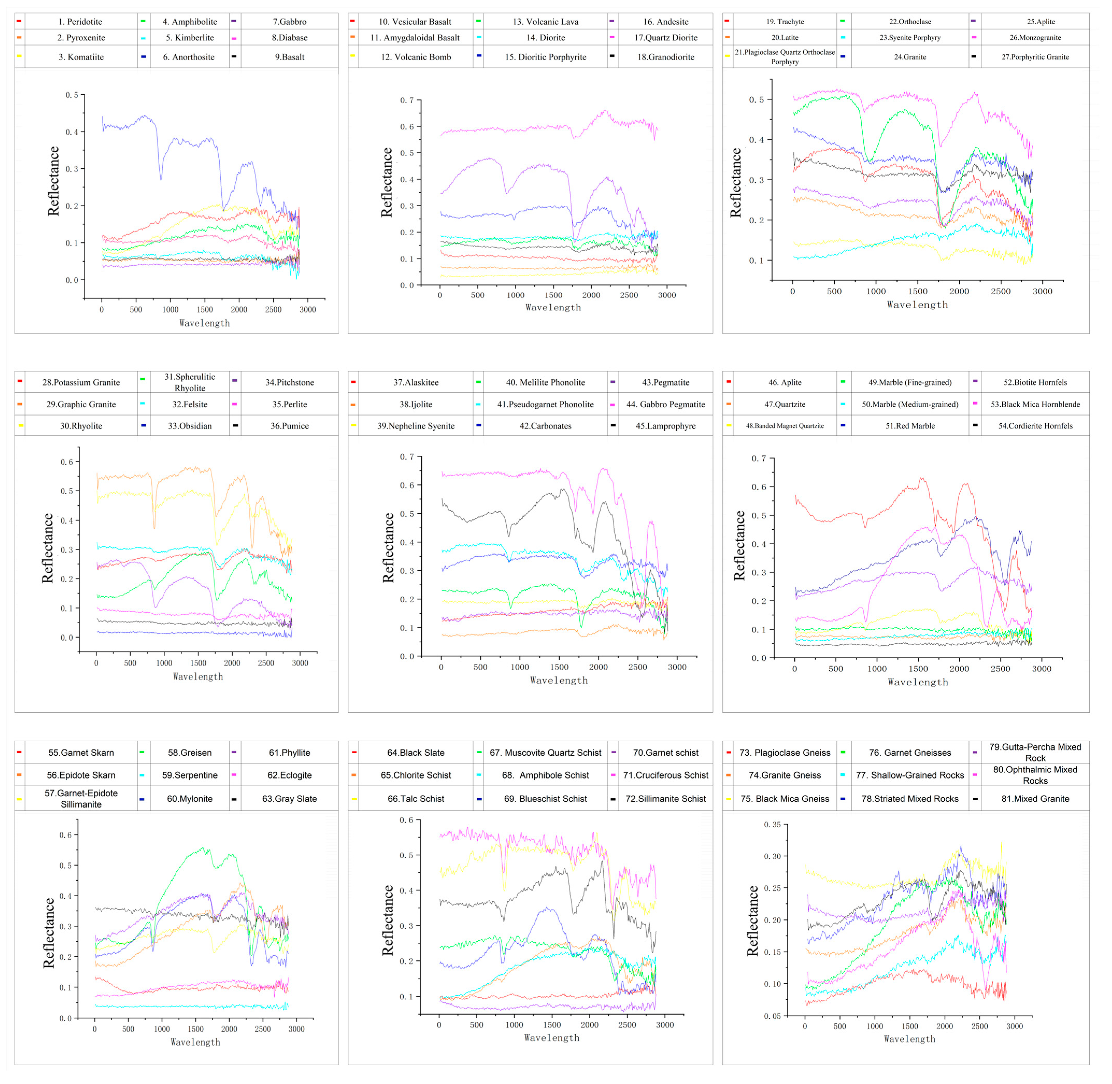
The first step during the data processing stage of the rock samples was to extract the spectral characteristics of 81 types of rocks from the preprocessed data and draw spectral curves (Figure 3).

2.3. Spectral Characteristics of Dataset HSRD-1.0

Among these (Figure 3), the spectral characteristics of rocks show obvious rock type dependence: igneous rocks are characterized by features such as the high reflectance of olivine, indicated by a strong absorption near 1000 nm, and pyroxene, showing double absorption peaks around 900 nm and 2000 nm in ferromagnesian rocks such as sample No. 1. Additionally, volcanic bombs (No. 12) and volcaniclastic rocks like pumice (No. 36), which are porous and glassy, exhibit low reflectance across the entire wavelength range and broadened water absorption peaks near 1400 nm. In contrast, the spectral features of metamorphic rocks are notably more complex. Fine-crystalline marble (No. 49) and medium-crystalline marble (No. 50) are primarily defined by the CO32− absorption peaks near 2300 nm in the near-infrared (NIR) band, with the peak depth correlating with the grain size of the rocks. For sillimanite-bearing contact metamorphic rocks, the epidote skarn (No. 56) and garnet-epidote sillimanite (No. 57) both exhibit spectral features influenced by the presence of chlorite minerals, which is the cause of their low reflectance and broadened water peaks in all bands. The core similarity between the spectral features of the striated mixed rock (No. 78) and the ophthalmic mixed rock (No. 80) lies in the fact that the spectral curves of both sillimanites show significant “sawtooth” features due to the alternate distribution of light bodies (feldspathic minerals) and dark bodies (ferromagnesian minerals). The spectral curves also show significant “jagged fluctuations”. These rocks’ spectral characteristics demonstrate a paradoxical duality—systematic intra-class regularity coupled with inter-class convergence—that both challenges diagnostic classification and validates the representativeness of experimental samples in encapsulating real-world lithological variability.

3. Method

3.1. Related Work

3.1.1. Two-Dimensional CNN

CNNs have shown significant advantages in the field of image spatial feature extraction by virtue of their local sensory fields and weight-sharing mechanism [38]. The two-dimensional convolutional neural network (2D-CNN) is a deep learning model designed for two-dimensional mesh data (e.g., images and video frames) that automatically extracts spatial features through convolutional operations, local connectivity, and weight-sharing mechanisms. Two-dimensional CNN has been widely applied in the field of computer vision, covering image classification, target detection, and image segmentation; it is also a core technology for efficiently processing two-dimensional spatial data. Given the unique characteristics of hyperspectral data, early studies modeled spatial neighborhood information employing 2D-CNN and used convolution kernels to capture local structural features such as rock texture and edges. Follow-up work further introduced a lightweight design to alleviate the overfitting problem in hyperspectral small-sample scenarios.
Given an input signal (usually a two-dimensional matrix such as an image) X, which is of size m × n, and a convolution kernel (also known as a filter) K, which is of size k × k , the convolution operation results in the output matrix Y, which is of size ( m k + 1 ) × ( n k + 1 ) (here, it is assumed that there is no padding, i.e., the padding is 0). The formula for each element Y [ i ] [ j ]   in the output matrix Y is
    Y i j = p = 0 k 1 q = 0 k 1 X i + p j + q × K p q

3.1.2. Recurrent Neural Network

A recurrent neural network (RNN) is a type of neural network designed for processing sequence data (e.g., text, speech, and time series), at the core of which are recurrent connections between neurons in the hidden layer that allow information to be passed in the temporal dimension, thus capturing temporal dependencies in the sequence [39].
It is widely used for the spectral sequence analysis of hyperspectral data due to its ability to model temporal dependencies. Classical LSTM [40] mitigates the long sequence gradient vanishing problem by introducing forgetting and input gates. In the field of hyperspectral rock classification, Agrawal & Govil [29] proposed a residual connection based on 1D CNN and LSTM to improve the difficulty in training caused by multi-layer LSTM stacking, and effectively identified most minerals such as alunite and calcite on the AVIRIS hyperspectral copper ore dataset, which is a typical application of RNN and its variants in this field. A gated recurrent unit (GRU) [41] further simplifies the gating mechanism by dynamically balancing the historical state and current input with an update gate and reset gate, which can balance efficiency and accuracy in spectral feature modeling. Equation (3) is the core formula of an RNN:
                    h t = σ W h h h t     1 + W x h h x t + b h
Here, h t denotes the hidden state at the current time step t, which summarizes the information from all previous time steps; h t     1 is the hidden state at the previous time step t     1 ; x t is the input at the current time step t; W h h and W x h are weight matrices that are used to linearly transform the hidden state and the inputs to capture the relationship between the inputs and the hidden state; b h is the bias term used to adjust the result after the linear transformation; and σ is an activation function, such as the hyperbolic tangent function tanh or the logistic function Sigmoid, which is used to introduce nonlinearities and enable the network to learn complex patterns.

3.2. Proposed Algorithm

This study proposes a dual-branch hyperspectral rock classification model that integrates 2D-CNN and GRU. Two-dimensional CNN extracts the spatial features of rocks through spectral dimensionality reduction and structural refinement to suppress redundant information, while the GRU models the temporal dependence of spectral sequences by using the gating mechanism to capture the subtle differences between bands. Both reduce the risk of overfitting through parameter optimization and introduce the AdaBoost algorithm to dynamically fuse two-branch features and preferentially strengthen the discriminant weight of spectrally confusing samples. The method simultaneously improves classification accuracy and generalization under small-sample conditions, effectively solves the classification ambiguity problem caused by the subtle differences in rock spectra, and provides an efficient and reliable technical solution for geological lithology identification (see Figure 4 for the schematic diagram).

3.2.1. A Framework for Hyperspectral Rock Classification Based on Bimodal Feature Synergy

To address the core challenges of hyperspectral rock image classification—namely subtle spectral differences and overfitting due to limited sample sizes—this study proposes a spatial-spectral bimodal cooperative learning framework. The framework features a dual-branch feature extraction network that integrates a 2D-CNN and a GRU. The 2D-CNN branch is based on PCA downscaling and streamlining structural design (e.g., compression of spectral channels, reduction in layers, and removal of pooling layers), which gives priority to the extraction of rock multi-scale spatial features (e.g., texture and edges) and improves the stability of training in small samples through batch normalization. In spectral sequence analysis, GRU branch is responsible for modeling the dynamic temporal dependencies within spectral sequences. The GRU branch uses the gating mechanism to model the dynamic temporal dependence of the sequence, and the reset and update gates collaboratively capture the cross-band local correlations and long-range spectral trends to enhance the sensitivity to subtle spectral differences. The dual-branch model effectively suppresses the risk of overfitting through parameter streamlining and complementary feature design, and it combines with the AdaBoost algorithm to adaptively fuse heterogeneous features to preferentially strengthen the discriminative weight of spectrally confusing lithological samples. Experimental results demonstrate that the framework enables effective collaborative optimization of spatial and spectral features, even with limited sample sizes. It significantly improves classification accuracy and model generalization, offering reliable technical support for intelligent lithological identification in geological exploration.

3.2.2. Two-Dimensional Convolutional Recurrent Neural Network

Through spatial-temporal bimodal feature extraction, the CNN and GRU are deeply integrated to provide the dual advantages of local detail perception and global temporal modeling. The 2D-CRNN model adopts a dual-path feature extraction architecture, and the 2D-CNN branch efficiently captures the spatial structural features of the rock image by streamlining the design of the number of convolutional channels and the number of layers while suppressing the overfitting risk. The RNN branch takes advantage of the temporal dependence modeling of the spectral sequence by the GRU to extract multi-level spectral response patterns [42].
The 2D-CNN branch, based on PCA dimensionality reduction, reduces the computational complexity by using PCA to reduce the spectral dimensions of the input data from 384 bands to 3 bands (as shown in Figure 5), eliminating redundant information to significantly improve model performance. The branch consists of two customized 2D convolutional layers that mine multi-scale rock spatial features from limited data, capturing key characteristics of rock images, such as edges, textures, and spatial positioning. To prevent overfitting, the spectral channels received by the 2D convolutional layer are compressed to three, and the number of convolutional layers and parallel loop cell layers is halved. At the same time, the pooling layer is omitted, thus maintaining a high spatial resolution. The convolutional layers leverage varying parameters and kernel sizes to extract features, integrating batch normalization and ReLU activation functions. The former performs normalization on small-sample data to stabilize data distributions, accelerate model convergence, and reduce gradient fluctuations, thereby enhancing stability; its regularization-like effect further mitigates overfitting. The latter introduces nonlinear factors to capture complex spectral relationships and address spectral confusion issues.
The RNN branch integrates 1D-CNN and GRU to capture spectral sequence features of rock images. In this framework, the spectral dimension of hyperspectral images is treated as temporal sequence features. When spectral data are fed into this branch, the 1D-CNN first extracts the central pixel block and performs dimensionality reduction while capturing local spectral features and patterns. Batch normalization layers and ReLU activation functions are appended after the convolutional layers, outputting preliminarily processed data. The GRU layer is designed to process the temporal sequence features of hyperspectral images along the spectral dimension. These features exhibit a dynamic and continuous nature, enabling the reflection of trends in rock spectral characteristics over time or wavelength-dependent variations. By modeling sequential dependencies, the GRU captures long-range spectral correlations and adaptively tracks gradual spectral shifts, enhancing the representation of subtle spectral patterns in geological samples.
Hyperspectral datasets are typically large and contain long spectral sequences, making it challenging to model spectral dependencies effectively. Traditional RNNs often struggle with capturing long-range relationships due to vanishing or exploding gradients. In contrast, GRU networks, with their streamlined gated mechanisms that efficiently regulate information flow, offer a more robust solution for modeling spectral-temporal relationships compared to LSTMs. The GRU layer improves the efficiency of training long-sequence data by simplifying the LSTM structure. The output from the GRU layer is processed through batch normalization and a tanh activation function, enhancing the model’s adaptability to data variations and nonlinear characteristics. Subsequently, the data undergo additional batch normalization and ReLU activation to optimize the final output.
The GRU employs gated mechanisms to model temporal dependencies in spectral sequences and extract multi-level spectral response patterns. A GRU features a more streamlined gating architecture than an LSTM with only an update gate and reset gate. Given a time step t, a small batch of inputs X t R n * d (n is the number of samples, and d is the number of inputs), and a hidden state H t     1 R n * h (h is the hidden unit dimension) of the previous time steps, the reset gate R t and the update gate Z t are calculated as
R t = s i g m o i d X t W x r + H t 1 W h r + b r
  Z t = s i g m o i d X t W x z + H t 1 W h z + b z
In Equation (4), W x r (x represents the input; r represents the reset gate) denotes the weight matrix from the input layer to the reset gate; W h r denotes the recursive weight from the hidden state to the reset gate, modeling the band correlation across time steps; and b r is the bias vector of the reset gate, which controls the default threshold for gate activation.
In Equation (5), W x z denotes the projection weights of inputs to the update gate, extracting diagnostic absorbing features; W h z denotes the recursive weights of hidden states to the update gate, maintaining the memory of key spectral features; and b z is the update gate bias. Positive initialization enhances the historical state retention tendency.
The Sigmoid function serves as the activation function to map values into the interval [0, 1], thereby regulating the gating mechanisms in the GRU. This ensures that the outputs of the reset gate R t and update gate Z t are constrained within the range [0, 1]. The GRU updates the hidden state by computing a candidate hidden state H ~ t , which is achieved through element-wise multiplication (shown as ⊙) between the reset gate output at the current time step t and the previous hidden state H t     1 . Specifically, the candidate hidden state H ~ t R n × h (where n is the batch size, and h is the hidden unit dimension) at time step t is formulated as
H ~ t = t a n h X t W x h + ( R t H t 1 ) W h h + b h
where W x h denotes the input-to-candidate-state projection weights, which capture localized spectral details by mapping raw spectral inputs to the hidden space. W h h represents the recurrent weights of the reset hidden state, modeling nonlinear interactions between spectral bands to refine temporal dependencies. b h is the candidate-state bias term, compensating for spectral baseline shifts and enhancing the adaptability of spectral feature representation.
This mechanism gives the GRU two key advantages. First, the reset gate R t explicitly captures local correlations between spectral bands—such as mineral absorption peaks—thereby increasing sensitivity to subtle spectral variations. Second, the update gate Z t adaptively balances long-range dependencies and short-term variations through weight optimization, effectively mitigating the vanishing gradient problem. This gating synergy makes the GRU particularly suitable for spatial-spectral joint modeling across hundreds of bands in hyperspectral data, providing theoretical guarantees for temporal feature extraction in dual-branch architectures.

3.2.3. AdaBoost Algorithm Integrated with Deep Learning Frameworks

After completing spatial-spectral dual-branch feature extraction, a key challenge in hyperspectral rock classification is how to effectively fuse these heterogeneous features and enhance classification robustness, especially under small-sample conditions. In the model constructed in this study, the two types of heterogeneous features are deeply fused by the fully connected layer to produce the initial classification probabilities. Here, weak classifiers are simple sub-modules with limited individual discriminative power—each focusing on specific local patterns within spatial or spectral features of hyperspectral rock data, with standalone performance slightly better than random guessing. The weight coefficients of each weak classifier are dynamically adjusted via error backpropagation by calculating the cross-entropy loss with respect to the true labels. This process enhances the weights of high-performing feature extraction paths while attenuating those of sub-optimal ones. Finally, a weighted voting mechanism integrates multi-path prediction results (i.e., summing each classifier’s output multiplied by its confidence weight), thereby achieving collaborative optimization of spatial-spectral features.
The iterative sample weighting mechanism of the AdaBoost algorithm directly addresses the key challenges in geological data by dynamically adjusting the training focus. In response to spectral confusion, the algorithm increases the weights of such difficult samples during consecutive iterations, compelling the model to deepen its ability to identify mineral absorption features. This weight allocation mechanism effectively mitigates the issue of class imbalance, while the confidence-weighted voting strategy significantly reduces cascading errors arising from spatial-spectral feature conflicts.
To further improve classification accuracy and generalization in hyperspectral rock classification, this study innovatively integrates the AdaBoost algorithm with a deep learning framework. This establishes a dual enhancement mechanism by dynamically adjusting both sample weights and model decision weights. Originally proposed by Freund and Schapire [43] in the 1990s, this algorithm’s core philosophy lies in iteratively adjusting sample weight distributions to force the model to persistently focus on hard samples, thereby improving discriminative capacity for fine-grained rock categories. Critically, the weak classifiers in this implementation are homogeneous architectures. Multiple identical convolutional recurrent neural networks (CRNNs). These CRNNs, constructed using the same CNN-GRU two-branch design described above, function as weak learners trained on iteratively re-weighted samples. This approach constitutes a homogeneous ensemble strategy—distinct from heterogeneous integrations (e.g., combining decision stumps with CRNNs)—where the base learner remains consistent across all iterations. Specifically, the model employs structurally invariant CRNNs whose parameters are optimized on dynamically adjusted sample distributions, eliminating cascaded errors from heterogeneous model fusion while maximizing feature decoupling capabilities for hyperspectral rock discrimination (see Figure 6 for the schematic diagram).
First, the sample weights are initialized. Assume that the dataset D contains M samples, and the initial weight of each sample is equal to w i 1 = 1 M ,   i.e., the weight of the ith sample in the first iteration round. Then, train a weak classifier c t x (t denotes round t) using the current sample weights and compute the weighted error rate r t of this weak classifier on the training set as
r t = i = 1 M w i t · I ( c t x i y i )
where I ( · )   is the indicator function, which takes the value of 1 when the prediction is wrong, and 0 otherwise. x i denotes the feature vector of the ith sample, so c t x i is the prediction value (±1) of the weak classifier for sample x i . y i , i.e., the input data, denotes the ith sample’s label, i.e., the output target that the model needs to predict.
The weight a t of the weak classifier is calculated according to the error rate obtained by the above calculation as
α t = l o g 1 r t r t
This weight reflects the importance of the weak classifier in the final decision; the lower the error rate, the higher the weight. Then, the sample weights are updated so that the weights of the misclassified samples are increased, as shown in Equation (9)
w i t + 1 = w i t e α t I y i c t x i
At each iteration, AdaBoost adjusts the sample weights according to the current classification results based on the fused feature map and improves the weights of misclassified samples. This not only enhances the model’s ability to handle noise and outliers but also helps it focus more effectively on relevant features when dealing with complex cases such as “spectral homogeneity with material heterogeneity” (SHMH) and “material consistency with spectral divergence” (MCSD), thereby improving overall model robustness.
When all the preset iteration rounds are completed, the algorithm calculates the corresponding combination coefficient α t for each weak classifier according to its error rate during training, and finally, the set of all weak classifiers is combined into a strong classifier through weighted linear superposition. Its mathematical expression is as Equation (10)
C x = s i g n t = 1 T α t · c t x
The sign (⋅) function serves as the signum operator, determining the final classification outcome. Here,   T   signifies the total iteration count, corresponding to the number of weak classifiers used during training.
The AdaBoost framework improves classification accuracy for geologically rare and spectrally similar rock types through strategic weight amplification of hard samples, concurrently suppressing overfitting while boosting model discriminative capability and operational robustness.
A deep ensemble network model, which includes a bi-branch network and AdaBoost algorithm, was designed in this study. The former makes full use of the advantages of bi-branch feature extraction to extract high discriminant space-spectrum features and realizes the balance optimization of accuracy and robustness in fine-grained rock classification tasks. The latter makes the model focus on difficult samples skillfully by iteratively adjusting sample weights, effectively improving the clarity of decision boundaries. Additionally, through a lightweight structural design, the model mitigates overfitting in small-sample scenarios and significantly improves overall performance in hyperspectral rock classification. This “sample-model” collaborative optimization strategy finally achieves a balanced optimization of accuracy and robustness in fine-grained rock classification.

4. Results and Discussion

4.1. Experimental Design

4.1.1. Datasets

This study established basic real labels for 81 types of rocks to allocate these categories to the training set, validation set, and test set. The number of pixel samples corresponding to each type of rock in the real labels was statistically analyzed and is presented in Table 1, thereby enhancing the accuracy and generalization ability of the supervised classification model.

4.1.2. Experimental Environment and Evaluation Criteria

The experiment was performed on a platform featuring an Intel(R) Xeon(R) Platinum 8255C CPU, an NVIDIA GeForce RTX 2080Ti GPU, and the Ubuntu 20.04 operating system. All experiments used PyTorch 1.11.0, Python 3.8, and CUDA 11.3. The specific Python modules and libraries included numpy 2.4.0, scikit-learn 1.3.2, and torch 1.11.0 + cu113.
The focus of this study is on the classification of hyperspectral rock images, and certain evaluation indicators are needed to reflect the classification effect when evaluating the classification results. Therefore, three commonly used indicators in this field were used to comprehensively evaluate the results: overall accuracy (OA), average accuracy (AA), and Kappa coefficient. OA represents the proportion of correctly classified samples to the total number of samples, and its calculation is as Equation (11):
O A = i = 1 n h i i i = 1 n N i
In Equation (12), n is the number of rock categories in the image, N i is the number of pixels in the ith rock category, and h i i is the number of pixels correctly classified in the ith category. AA is the sum of the sample proportion of each category relative to the total number of samples, divided by the number of categories.
A A = 1 n i = 1 n h i i N i  
The Kappa coefficient is an indicator of consistency that can be used to measure the validity of a classification. It is calculated using Equation (13)
K a p p a = N i = 1 r x i i i = 1 r x i + x + i N 2 i = 1 r x i + x + i
where N is the total number of samples;   r is the number in the confusion matrix; x i + and x + i   are the sum of the elements in row i and column i of the confusion matrix, respectively; and x i i   is the value of column i in row i of the confusion matrix.

4.1.3. Experimental Setup

In the proposed C-RNN-AdaBoost model, the AdaBoost algorithm uses 10 decision stumps as weak classifiers, and the weights of the C-RNN model are initialized by the He normal distribution, while the bias term is set to zero, and the layer without the bias term is not initialized. The Adam algorithm was used in the optimization process, with the initial learning rate set to 0.001; dynamic adjustment was implemented to adapt to the change in the learning rate during the training process.
In terms of data processing, a five-fold cross-validation method was used in this study. In each iteration, 20% of the pixels were randomly selected as the training set, 70% for testing, and the remaining 10% for validation. And this data partitioning method helps evaluate the generalization ability of the model, but it may also lead to differences in sample distribution between different folds, which can affect the consistency of model performance.
The experimental results (as shown in Table 2) indicated that when using C-RNN to classify 81 types of rocks individually, there were significant differences in training accuracy between different folds. This was mainly attributed to the reduction in sample size and the uneven distribution of features. In addition, the decision stumps in AdaBoost performed poorly in capturing complex feature relationships, especially in multi-class tasks that require fine differentiation, exposing the limitations of traditional machine learning methods in such tasks.

4.1.4. Effect of the Number of Training Rounds on Classification Accuracy

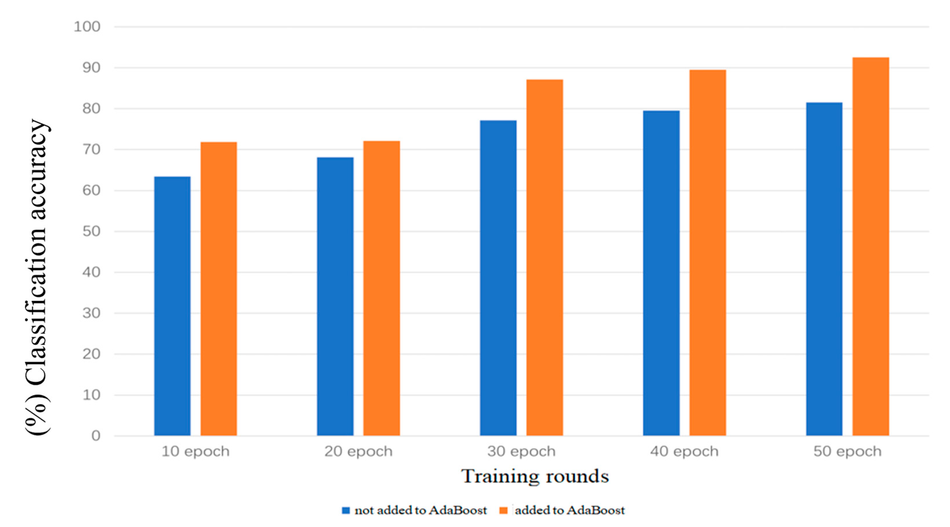
Through experiments with different training rounds (10, 20, 30, 40, and 50 rounds) —involving dynamic adjustment of the initial learning rate (0.001) by a factor of 10 when validation accuracy stagnated, moderate increases in weight decay (from 1 × 10⁻⁵ to 5× 10⁻⁵) to mitigate overfitting, and a stable batch size of 32. The specific effect of the AdaBoost algorithm on model performance was analyzed. The experimental results (as shown in Figure 7) showed that the model incorporating AdaBoost demonstrated higher classification accuracy in all tested training rounds. The accuracy of both types of models improved significantly after 20 rounds, but after more than 40 rounds, this improvement became limited. To make rational use of computing resources, this experiment was terminated after 50 rounds of training.

4.1.5. Effect of the Number of Weak Classifiers on Classification Accuracy

To investigate the effect of the number of weak classifiers on the classification accuracy of the AdaBoost algorithm, experiments were conducted using one, three, five, and seven classifiers. The experimental results (as shown in Table 3. Comparison of classification accuracy for different numbers of weak classifiers in the model.) indicated that the classification accuracy was optimal when using three classifiers, although the training time increased compared with using one classifier, and overfitting did not occur. As the number of classifiers increased further, the classification accuracy did not significantly improve but rather decreased, and the model began to overfit and consume more resources. Therefore, subsequent experiments all used three classifiers for training.

4.1.6. Effect of RNN Branch on Classification Accuracy

The proposed C-RNN-AdaBoost model enhances spectral feature extraction through the GRU gating mechanism, highlighting the key role of spectral information in rock classification. To verify its effectiveness, three typical bi-branched space-spectral fusion models (2D-CNN-BiRNN-AdaBoost, 2D-1D CNN-AdaBoost, and 2D-LSTM-AdaBoost) [29,44,45] were used for comparison, and the OA, AA and Kappa coefficient of the proposed model are all higher were higher (as shown in Table 4). All models were trained on 20% data and cross-validated with a 5% fold. In addition, by simplifying the network structure and reducing the number of parameters, the C-RNN-AdaBoost model significantly reduces the computing resources and time consumption while maintaining efficient classification.
Specifically, although the bidirectional recurrent neural network (BiRNN) enhances the ability to perceive context, it performs poorly in classification tasks, exhibiting gradient anomalies and defects in long-range information processing. LSTM alleviates the problem of gradient vanishing through the gating mechanism, which significantly improves the classification accuracy. The 1D-CNN branch has significant advantages in local feature extraction, and its classification effect is similar to that of the model proposed in this study. However, the 1D-CNN needs more training parameters for training, resulting in a large consumption of computing resources and time.
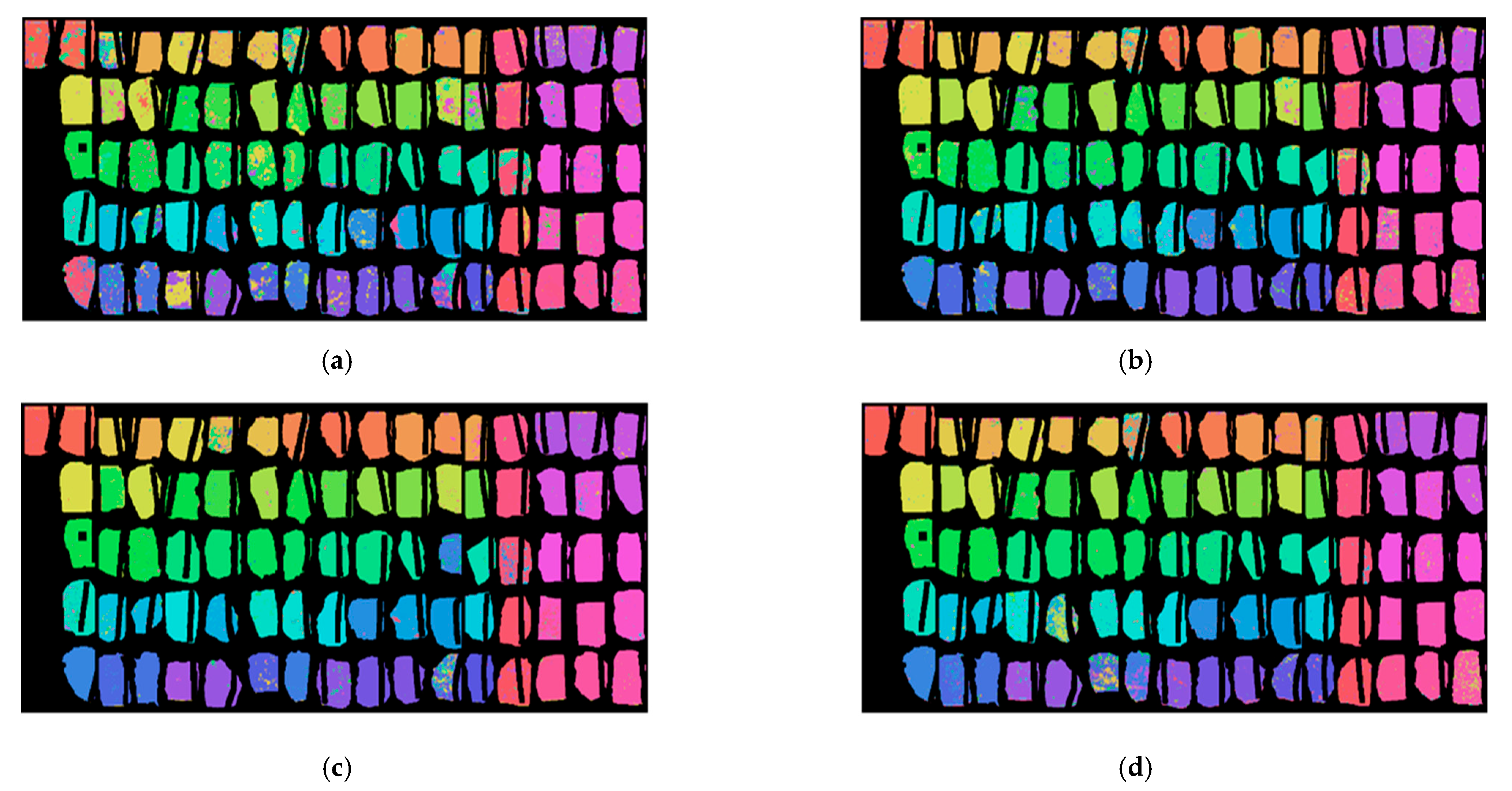
The text model adopts a simplified GRU structure, which only contains two gates, reducing the number of parameters compared with the LSTM’s three gates, thereby lowering the computational complexity. The update gate mechanism of the GRU achieves an effective balance between long-term and short-term dependence, and it further improves the classification accuracy. The classification effect diagram of the four algorithms shown in Figure 8 indicates that the proposed model had higher smoothness in rock classification than other comparative models. Furthermore, there were fewer misclassified pixels, which verifies the high efficiency and robustness of the proposed model in complex rock classification tasks.

4.2. Comparison and Discussion of Experimental Results

To evaluate the effectiveness of the rock classification algorithm introduced in this study, several mainstream hyperspectral image classification algorithms (including 3D-CNN, Bi-CLSTM, SSRN, and DenseNet) were selected for comparative analysis [46,47,48,49]. All models use a five-fold cross-validation method to divide the training, validation, and test data. The proposed model showed the highest classification accuracy for the dataset containing 81 types of rock as shown in Table 5.
The 3D-CNN and SSRN belong to the traditional 3D convolutional single-branch cascade model, and the SSRN is better than the 3D-CNN because it introduces the residual network structure of skipping connections, which improves the stability and classification accuracy of training. Bi-CLSTM combines the advantages of bidirectional LSTM and convolutional LSTM to extract local features better, but its performance is degraded due to the significant difference in the distribution of training and test data. DenseNet achieved a classification accuracy second only to the proposed model by using a dense connection mechanism, allowing each layer to directly access the feature information of all preceding layers.
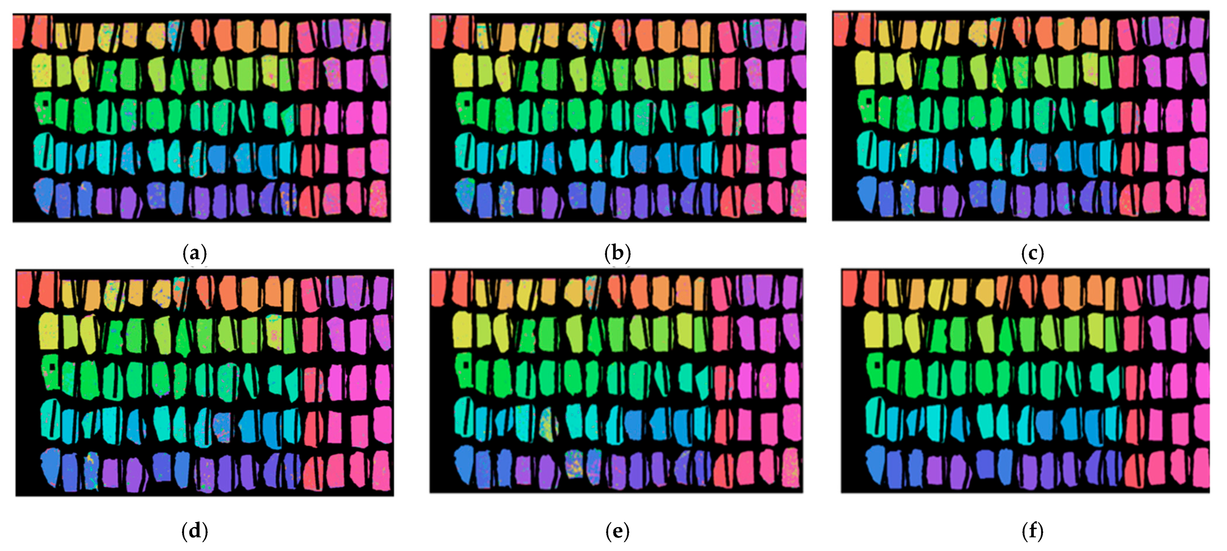
As shown in Figure 9, the proposed model (e) had the least misfraction of pixels compared with (a) 3D-CNN, (b) Bi-CLSTM, (c) SSRN, and (d) DenseNet, especially in the transition region at the rock edges.

4.3. Analysis and Discussion of Typical Samples of Metamorphic Rock

4.3.1. Identification of Typical and Easily Confused Metamorphic Rock

For spectrally similar lithological assemblages, including fine-grained marble (sample 49) and medium-crystalline marble (sample 50), epidote skarn (sample 56) and its garnet-bearing variant (sample 57), amphibole-dominant lithologies (samples 68 and 73), and migmatitic complexes like garnet schist and sillimanite schist (70/72), the model exhibited robust multi-scale feature extraction capabilities, achieving classification accuracies above 98.6% for all critical sample sets. Detailed classification metrics for these four representative groups are provided in Table 6, and the corresponding spectral profiles are visualized in Figure 10.

4.3.2. Class Identification of Typical Metamorphic Rock

The confusion matrix intuitively shows the predicted vs. actual results across categories. Confusion matrix heatmaps visualizing prediction results for five distinct models are displayed in Figure 11.
Cordierite hornfels and granites have similar spectral characteristics and highly overlapping mineral assemblages, which increases the classification difficulty:
Spectral curve similarity: Cordierite formation is intrinsically linked to biotite dehydration melting reactions. This petrogenetic process induces significant spectral overlap between cordierite-dominant hornfels and granite in the 2200–2400 nm range, where overlapping hydroxyl (OH) and ferrous iron (Fe2+) absorption features create nearly identical reflectance curve morphologies. Additionally, these lithologies show comparable full width at half maximum (FWHM) values for their broad absorption features in the 1000–1300 nm region. Such spectral convergence hinders deep learning models from resolving diagnostic mineralogical signatures, leading to blurred classification boundaries and a significant increase in error rates.
Mineralogical composition overlap: Both rock types share common components such as quartz and mafic minerals (e.g., cordierite and biotite), leading to similar spectral responses due to Fe2+ and Al-OH absorption features. Quantitative analyses reveal over 20% error in mineral abundance estimation between them. Weathered secondary minerals (e.g., limonite and kaolinite) and mixed image element interference (>40% mixing probability at 30 m resolution) further confound the primary spectral-compositional correlation.
In the model developed in this study, the reduced brightness of the highlighted regions (indicated by the red box) indicates that most of the previously confused samples were correctly classified. This demonstrates the model’s higher OA and improved classification performance.
Nevertheless, the proposed model exhibits persisting limitations in specific lithological identifications. Notably, all benchmark models consistently misclassified sample 36 (pumice), with the 3D-CNN erroneously identifying its primary lithology as sample 13 (volcanic lava). This confusion arises from an 82% spectral overlap in low-frequency band trends between these lithotypes (Figure 10). The issue is exacerbated when models focus more on extracting spatial features—such as textural patterns, edge contours, or pixel distribution structures within the rock image—rather than prioritizing discriminative spectral signatures that could distinguish them.
Furthermore, both our model and comparative architectures partially mislabeled regions of sample 36 (pumice) as sample 59 (serpentinite). Spectral curve analysis revealed reflectance divergence of only 3.6% in high-frequency bands between these lithologies, highlighting the persistent challenge of differentiating subtle spectral variations below a 5% contrast threshold—a critical performance boundary in hyperspectral petrological classification.
Mineralogically, this challenge arises because pumice (sample 36), a porous glassy volcaniclastic rock, and serpentinite (sample 59), dominated by hydrous serpentine, share convergent spectral drivers: both contain hydroxyl (OH) groups (from adsorbed water in pumice’s glassy matrix and serpentine’s crystal structure) causing overlapping near-infrared absorption. Their fine-grained textures further minimize reflectance contrasts, making subtle <5% differences indistinct to models.

5. Conclusions

In this study, 81 rock types were classified using a series of network models designed to fully exploit both the spatial and spectral information of rocks and minerals. Ultimately, a deep learning model combining a CNN and an RNN was proposed for the classification of hyperspectral rock images. The AdaBoost integration demonstrably enhanced model stability, reducing the standard deviation of overall accuracy (OA) from 32.85% in the base C-RNN model to 7.44% in the CRNN-AdaBoost ensemble. By fully leveraging the multi-dimensional information in hyperspectral rock images, the model reduces the occurrence of “spectral homogeneity with material heterogeneity (SHMH)” and “material consistency with spectral divergence (MCSD)” phenomena, thereby significantly enhancing classification accuracy. By introducing the AdaBoost algorithm, the stability and generalization ability of the model were enhanced, especially in cases with few samples and diverse categories. This approach effectively reduces overfitting and improves discriminative power, thereby enhancing the classification accuracy across the 81 types of fine-grained rocks. However, the misjudgment of spectrally highly similar samples, such as No. 36 (pumice) and No. 59 (serpentine), still exposes the insufficient sensitivity of the model to subtle feature differences. Future work will focus on the following three aspects. First, we will introduce prior knowledge of mineral composition to construct a spectral decoupling network, enhancing the ability to distinguish spectrally similar categories. Second, we will adapt to real-time field detection requirements through dynamic pruning and quantization compression of model parameters. Third, we will integrate multi-modal data such as LiDAR and micro-imaging data to build a cross-scale rock analysis framework, further breaking through the spectral limitations of single data sources and promoting the development of geological interpretation toward multi-dimensional intelligence.

Author Contributions

Conceptualization was done by S.X., Y.Q. and S.C. S.C. was responsible for Methodology and Software. Validation was carried out by Y.Q. Formal analysis was done by W.W. Y.Q. and S.X. wrote the original draft, while W.W. and S.X. were responsible for writing—review and editing. Visualization was done by S.X. All authors edited the paper. All authors have read and agreed to the published version of the manuscript.

Funding

This research was funded by the National Natural Science Foundation of China (No. 61701153 and No. 41402304) and Zhejiang Provincial Natural Science Foundation of China (LQ13D020002).

Data Availability Statement

Dataset details and downloads are available at https://uwrl.hznu.edu.cn/c/2023-02-24/2805144.shtml (accessed on 27 August 2024).

Conflicts of Interest

The authors declare no conflicts of interest.

References

  1. Karimpouli, S.; Tahmasebi, P. Segmentation of digital rock images using deep convolutional autoencoder networks. Comput. Geosci. 2019, 126, 142–150. [Google Scholar] [CrossRef]
  2. Guo, W.; Dong, C.; Lin, C.; Wu, Y.; Zhang, X.; Liu, J. Rock physical modeling of tight sandstones based on digital rocks and reservoir porosity prediction from seismic data. Front. Earth Sci. 2022, 10, 932929. [Google Scholar] [CrossRef]
  3. Houshmand, N.; Goodfellow, S.; Esmaeili, K.; Calderón, J.C.O. Rock type classification based on petrophysical, geochemical, and core imaging data using machine and deep learning techniques. Appl. Comput. Geosci. 2022, 16, 100104. [Google Scholar] [CrossRef]
  4. Li, W.; Yin, G.; Yu, H.; Liu, X. The Yanshanian granites and associated Mo-polymetallic mineralization in the Xiangcheng-Luoji area of the Sanjiang-Yangtze conjunction zone in Southwest China. Acta Geol. Sin.—Engl. Ed. 2014, 88, 1742–1756. [Google Scholar] [CrossRef]
  5. Ferrero, S.; Bartoli, O.; Cesare, B.; Salvioli-Mariani, E.; Acosta-Vigil, A.; Cavallo, A.; Groppo, C.; Battiston, S. Microstructures of melt inclusions in anatectic metasedimentary rocks. J. Metamorph. Geol. 2012, 30, 303–322. [Google Scholar] [CrossRef]
  6. Xu, Y.; Ma, H.; Peng, S. Study on identification of altered rock in hyperspectral imagery using spectrum of field object. Ore Geol. Rev. 2014, 56, 584–595. [Google Scholar] [CrossRef]
  7. Zhao, J.; Wang, G.; Zhou, B.; Ying, J.; Liu, J. Exploring an application-oriented land-based hyperspectral target detection framework based on 3D–2D CNN and transfer learning. EURASIP J. Adv. Signal Process. 2024, 2024, 37. [Google Scholar] [CrossRef]
  8. Transon, J.; D’Andrimont, R.; Maugnard, A.; Defourny, P. Survey of Hyperspectral Earth Observation Applications from Space in the Sentinel-2 Context. Remote Sens. 2018, 10, 157. [Google Scholar] [CrossRef]
  9. Jakob, S.; Zimmermann, R.; Gloaguen, R. The need for accurate geometric and radiometric corrections of drone-borne hyperspectral data for mineral exploration: MEPHySTo—A toolbox for pre-processing drone-borne hyperspectral data. Remote Sens. 2017, 9, 88. [Google Scholar] [CrossRef]
  10. Paoletti, M.E.; Haut, J.M.; Plaza, J.; Plaza, A. Deep&Dense Convolutional Neural Network for Hyperspectral Image Classification. Remote Sens. 2018, 10, 1454. [Google Scholar] [CrossRef]
  11. Zhang, X.; Li, P. Lithological mapping from hyperspectral data by improved use of spectral angle mapper. Int. J. Appl. Earth Obs. Geoinf. 2014, 31, 95–109. [Google Scholar] [CrossRef]
  12. Breiman, L. Random forests. Mach. Learn. 2001, 45, 5–32. [Google Scholar] [CrossRef]
  13. Kanungo, T.; Mount, D.M.; Netanyahu, N.S.; Piatko, C.D.; Silverman, R.; Wu, A.Y. An efficient k-means clustering algorithm: Analysis and implementation. IEEE Trans. Pattern Anal. Mach. Intell. 2002, 24, 881–892. [Google Scholar] [CrossRef]
  14. Ghezelbash, R.; Maghsoudi, A.; Shamekhi, M.; Pradhan, B.; Daviran, M. Genetic algorithm to optimize the SVM and K-means algorithms for mapping of mineral prospectivity. Neural Comput. Appl. 2023, 35, 719–733. [Google Scholar] [CrossRef]
  15. Tessier, J.; Duchesne, C.; Bartolacci, G. A machine vision approach to on-line estimation of run-of-mine ore composition on conveyor belts. Miner. Eng. 2007, 20, 1129–1144. [Google Scholar] [CrossRef]
  16. Tripathi, P.; Garg, R.D. Potential of DESIS and PRISMA hyperspectral remote sensing data in rock classification and mineral identification: A case study for Banswara in Rajasthan, India. Environ. Monit. Assess. 2023, 195, 575. [Google Scholar] [CrossRef] [PubMed]
  17. Hughes, G. On the mean accuracy of statistical pattern recognizers. IEEE Trans. Inf. Theory 1968, 14, 55–63. [Google Scholar] [CrossRef]
  18. Kilickaya, S.; Ahishali, M.; Sohrab, F.; Ince, T.; Gabbouj, M. Hyperspectral image analysis with subspace learning-based one-class classification. In Proceedings of the 2023 Photonics & Electromagnetics Research Symposium (PIERS), Prague, Czech Republic, 3–6 July 2023; pp. 953–959. [Google Scholar] [CrossRef]
  19. Güler, E.; Kakız, M.T.; Günay, F.B.; Şanal, B.; Çavdar, T. Kapalı mekan ortamında 1D-CNN kullanarak yapılan doluluk tespiti sınıflandırması. Karadeniz Fen Bilim. Derg. 2023, 13, 60–71. [Google Scholar] [CrossRef]
  20. Yang, J.; Chang, B.; Zhang, Y.; Luo, W.; Ge, S.; Wu, M. CNN coal and rock recognition method based on hyperspectral data. Int. J. Coal Sci. Technol. 2022, 9, 63. [Google Scholar] [CrossRef]
  21. Zhang, C.; Yi, M.; Ye, F.; Xu, Q.; Li, X.; Gan, Q. Application and Evaluation of Deep Neural Networks for Airborne Hyperspectral Remote Sensing Mineral Mapping: A Case Study of the Baiyanghe Uranium Deposit in Northwestern Xinjiang, China. Remote Sens. 2022, 14, 5122. [Google Scholar] [CrossRef]
  22. Jiang, T.; Wang, X.J. Hyperspectral images classification based on fusion features derived from 1D and 2D convolutional neural network. Int. Arch. Photogramm. Remote Sens. Spat. Inf. Sci. 2020, 42, 335–341. [Google Scholar] [CrossRef]
  23. Sinaice, B.B.; Kawamura, Y.; Kim, J.; Okada, N.; Kitahara, I.; Jang, H. Application of deep learning approaches in igneous rock hyperspectral imaging. In Proceedings of the 28th International Symposium on Mine Planning and Equipment Selection—MPES 2019, Perth, Australia, 2–4 December 2019; Topal, E., Ed.; Springer: Cham, Switzerland, 2020; pp. 347–356. [Google Scholar] [CrossRef]
  24. Ge, W.; Cheng, Q.; Tang, Y.; Jing, L.; Gao, C. Lithological classification using Sentinel-2A data in the Shibanjing ophiolite complex in Inner Mongolia, China. Remote Sens. 2018, 10, 638. [Google Scholar] [CrossRef]
  25. Bozga, M.; Maler, O.; Tripakis, S. Efficient verification of timed automata using dense and discrete time semantics. In Correct Hardware Design and Verification Methods; Pierre, L., Kropf, T., Eds.; Springer: Berlin/Heidelberg, Germany, 1999; pp. 125–141. [Google Scholar] [CrossRef]
  26. Dang, L.; Pang, P.; Zuo, X.; Liu, Y.; Lee, J. A Dual-Path Small Convolution Network for Hyperspectral Image Classification. Remote Sens. 2021, 13, 3411. [Google Scholar] [CrossRef]
  27. Hussain, M.; Bird, J.J.; Faria, D.R. A study on CNN transfer learning for image classification. In Advances in Computational Intelligence Systems: UKCI 2018; Lotfi, A., Bouchachia, H., Gegov, A., Langensiepen, C., McGinnity, M., Eds.; Springer: Cham, Switzerland, 2019; Volume 84, pp. 199–212. [Google Scholar] [CrossRef]
  28. Zhao, H.; Deng, K.; Li, N.; Wang, Z.; Wei, W. Hierarchical Spatial-Spectral Feature Extraction with Long Short Term Memory (LSTM) for Mineral Identification Using Hyperspectral Imagery. Sensors 2020, 20, 6854. [Google Scholar] [CrossRef] [PubMed]
  29. Agrawal, N.; Govil, H. A deep residual convolutional neural network for mineral classification. Adv. Space Res. 2023, 71, 3186–3202. [Google Scholar] [CrossRef]
  30. Liu, Y.; Wu, X.; Teng, Q.; He, H. Mineral identification of rock thin section images based on improved SKnet and Bi-GRU. Intell. Comput. Appl. 2023, 13, 104–111. [Google Scholar] [CrossRef]
  31. Okada, N.; Maekawa, Y.; Owada, N.; Haga, K.; Shibayama, A.; Kawamura, Y. Automated Identification of Mineral Types and Grain Size Using Hyperspectral Imaging and Deep Learning for Mineral Processing. Minerals 2020, 10, 809. [Google Scholar] [CrossRef]
  32. Galdames, F.J.; Perez, C.A.; Estévez, P.A.; Adams, M. Rock lithological instance classification by hyperspectral images using dimensionality reduction and deep learning. Chemom. Intell. Lab. Syst. 2022, 224, 104538. [Google Scholar] [CrossRef]
  33. Li, D.; Zhao, J.; Ma, J. Experimental studies on rock thin-section image classification by deep learning-based approaches. Mathematics 2022, 10, 2317. [Google Scholar] [CrossRef]
  34. Zhang, Z.; Zheng, C.; Liang, C.; Santosh, M.; Hao, J.; Dong, L.; Hou, J.; Hou, F.; Li, M. Metamorphism and P-T Evolution of High-Pressure Granulites from the Fuping Complex, North China Craton. Minerals 2024, 14, 138. [Google Scholar] [CrossRef]
  35. Barbey, P.; Marignac, C.; Montel, J.M.; Macaudière, J.; Gasquet, D.; Jabbori, J. Cordierite growth textures and the conditions of genesis and emplacement of crustal granitic magmas: The Velay granite complex (Massif Central, France). J. Petrol. 1999, 40, 1425–1441. [Google Scholar] [CrossRef]
  36. Regmi, K.R. Petrogenesis of the augen gneisses from Mahesh Khola section, Central Nepal. Bull. Dep. Geol. 2008, 11, 13–22. [Google Scholar] [CrossRef]
  37. Karimzadeh, Z.; Tangestani, M.H. Application of WorldView-3 data in alteration mineral mapping in Chadormalu area, central Iran. Int. Arch. Photogramm. Remote Sens. Spat. Inf. Sci. 2019, 42, 589–596. [Google Scholar] [CrossRef]
  38. LeCun, Y.; Boser, B.; Denker, J.S.; Henderson, D.; Howard, R.E.; Hubbard, W.; Jackel, L.D. Backpropagation applied to handwritten zip code recognition. Neural Comput. 1989, 1, 541–551. [Google Scholar] [CrossRef]
  39. Zaremba, W.; Sutskever, I.; Vinyals, O. Recurrent neural network regularization. arXiv 2014. [Google Scholar] [CrossRef]
  40. Hochreiter, S.; Schmidhuber, J. Long short-term memory. Neural Comput. 1997, 9, 1735–1780. [Google Scholar] [CrossRef]
  41. Dey, R.; Salem, F.M. Gate-variants of gated recurrent unit (GRU) neural networks. In Proceedings of the 2017 IEEE 60th International Midwest Symposium on Circuits and Systems (MWSCAS), Boston, MA, USA, 6–9 August 2017; pp. 1597–1600. [Google Scholar] [CrossRef]
  42. Chung, J.; Gulcehre, C.; Cho, K.; Bengio, Y. Empirical evaluation of gated recurrent neural networks on sequence modeling. arXiv 2014. [Google Scholar] [CrossRef]
  43. Freund, Y.; Schapire, R.E. A decision-theoretic generalization of on-line learning and an application to boosting. J. Comput. Syst. Sci. 1997, 55, 119–139. [Google Scholar] [CrossRef]
  44. Schuster, M.; Paliwal, K.K. Bidirectional recurrent neural networks. IEEE Trans. Signal Process. 1997, 45, 2673–2681. [Google Scholar] [CrossRef]
  45. Alrebdi, N.; Al-Shargabi, A.A. Emotional state prediction based on EEG signals using ensemble methods. Int. J. Adv. Comput. Sci. Appl. 2023, 14, 123. [Google Scholar] [CrossRef]
  46. Li, Y.; Zhang, H.; Shen, Q. Spectral–Spatial Classification of Hyperspectral Imagery with 3D Convolutional Neural Network. Remote Sens. 2017, 9, 67. [Google Scholar] [CrossRef]
  47. Liu, Q.; Zhou, F.; Hang, R.; Yuan, X. Bidirectional-convolutional LSTM based spectral-spatial feature learning for hyperspectral image classification. Remote Sensing 2017, 9, 1330. [Google Scholar] [CrossRef]
  48. Zhong, Z.; Li, J.; Luo, Z.; Chapman, M. Spectral–spatial residual network for hyperspectral image classification: A 3-D deep learning framework. IEEE Trans. Geosci. Remote Sens. 2018, 56, 847–858. [Google Scholar] [CrossRef]
  49. Huang, G.; Liu, Z.; Van Der Maaten, L.; Weinberger, K.Q. Densely connected convolutional networks. In Proceedings of the 2017 IEEE Conference on Computer Vision and Pattern Recognition (CVPR), Honolulu, HI, USA, 21–26 July 2017; pp. 2261–2269. [Google Scholar] [CrossRef]
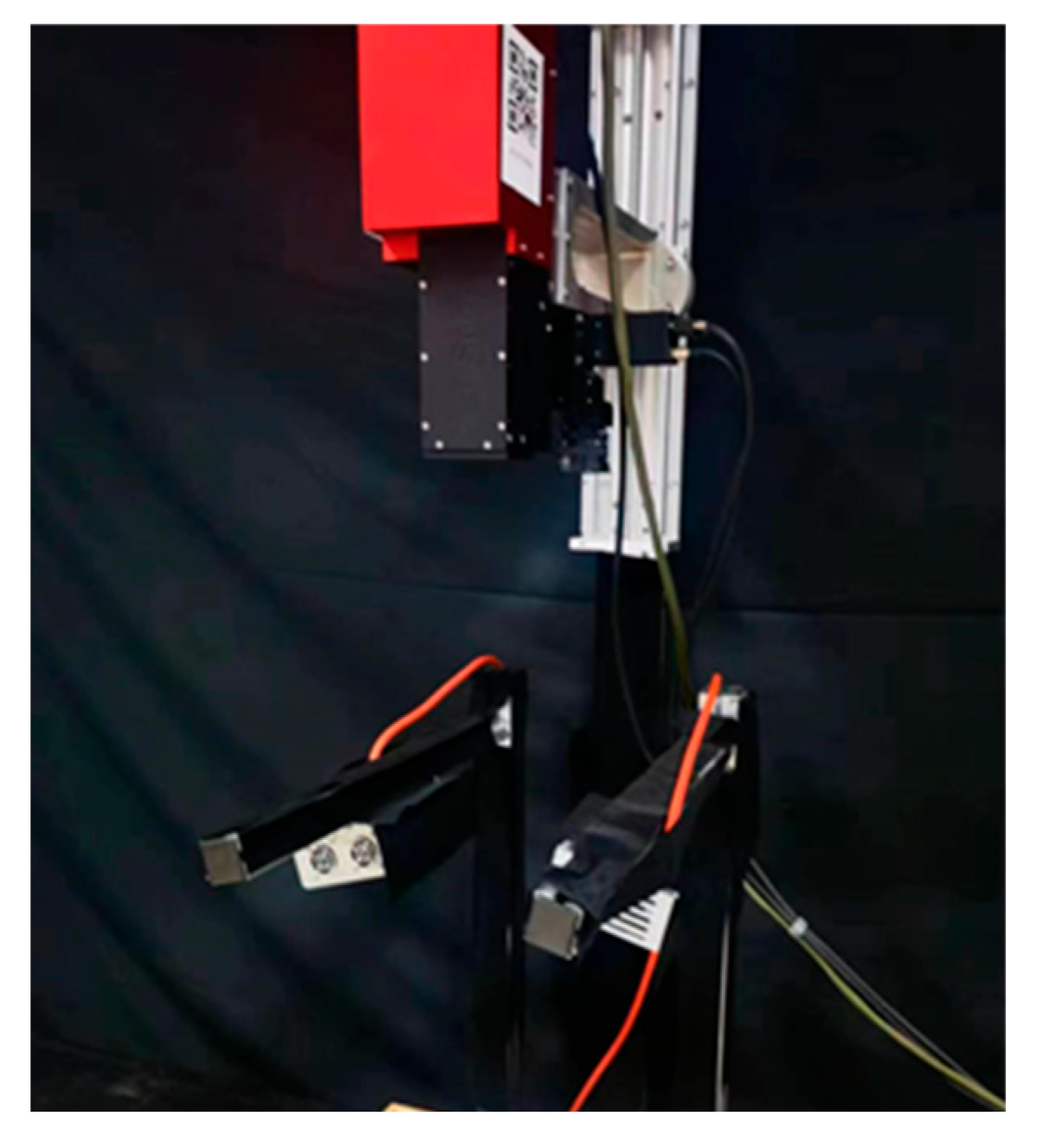
Figure 1. HySpex hyperspectral sensor.
Minerals 15 00844 g001
Figure 2. Dataset HSRD-1.0. (a) Classification of 81 rock samples, (b) false color composite image of samples, and (c) true labels after corrosion.
Minerals 15 00844 g002
Figure 3. Spectral curves of 81 rock types.
Minerals 15 00844 g003
Figure 4. Deep integration network diagram.
Minerals 15 00844 g004
Figure 5. Two-dimensional convolutional recurrent neural network module.
Minerals 15 00844 g005
Figure 6. Schematic diagram of the AdaBoost algorithm.
Minerals 15 00844 g006
Figure 7. Comparison of overall classification accuracy between two models with different training rounds.
Minerals 15 00844 g007
Figure 8. Classification renderings of models under different RNN branches on the dataset containing 81 types of rock: (a) 2D-BRNN-AdaBoost, (b) 2D-LSTM-AdaBoost, (c) 2D-1D CNN-AdaBoost, and (d) proposed model.
Minerals 15 00844 g008
Figure 9. Classification renderings of different models on the dataset containing 81 types of rock: (a) 3D-CNN, (b) Bi-CLSTM, (c) SSRN, (d) DenseNet, (e) proposed model, and (f) real label.
Minerals 15 00844 g009
Figure 10. Spectral characteristics of metamorphic subtypes: (a) marble (fine-grained; No. 49, green) vs. marble (medium-grained; No. 50, blue); (b) epidote skarn (No. 56, orange) vs. garnet-epidote sillimanite rock (No. 57, yellow); (c) amphibole schist (No. 68, blue) vs. plagioclase gneiss (No. 73, red); (d) banded migmatite (No. 78, purple) vs. sillimanite schist (No. 72, black); (e) pumice (No. 36, red) vs. serpentine (No. 59, green), and (f) volcanic lava (No. 13,blue) vs. pumice (No. 36, red).
Minerals 15 00844 g010
Figure 11. Visualization of confusion matrix thermodynamics for different models: (a) 3D CNN, (b) Bi-CLSTM, (c) SSRN, (d) DenseNet, and (e) proposed model.
Minerals 15 00844 g011
Table 1. Eighty-one types of rock labels corresponding to color and pixel sample number.
Rock NameClassSamplesRock NameClassSamples
PeridotiteMinerals 15 00844 i001   14986Pseudoleucite PhonoliteMinerals 15 00844 i002   415014
PyroxeniteMinerals 15 00844 i003   25519CarbonatiteMinerals 15 00844 i004   424576
KomatiiteMinerals 15 00844 i005   35740PegmatiteMinerals 15 00844 i006   436018
AmphiboliteMinerals 15 00844 i007   44837Gabbroic PegmatiteMinerals 15 00844 i008   444631
KimberliteMinerals 15 00844 i009   56548LamprophyreMinerals 15 00844 i010   455078
AnorthositeMinerals 15 00844 i011   65404ApliteMinerals 15 00844 i012   465045
GabbroMinerals 15 00844 i013   75472QuartziteMinerals 15 00844 i014   474175
DiabaseMinerals 15 00844 i015   84166Banded Magnetite QuartziteMinerals 15 00844 i016   484722
BasaltMinerals 15 00844 i017   93747Marble (Fine-grained)Minerals 15 00844 i018   492771
Vesicular BasaltMinerals 15 00844 i019   104296Marble (Medium-grained)Minerals 15 00844 i020   505699
Amygdaloidal BasaltMinerals 15 00844 i021   112906Red MarbleMinerals 15 00844 i022   515551
Volcanic BombMinerals 15 00844 i023   124739Andalusite HornfelsMinerals 15 00844 i024   523969
Volcanic LavaMinerals 15 00844 i025   132945Biotite HornfelsMinerals 15 00844 i026   534983
DioriteMinerals 15 00844 i027   146163Cordierite HornfelsMinerals 15 00844 i028   543479
Diorite PorphyryMinerals 15 00844 i029   154923Garnet SkarnMinerals 15 00844 i030   554842
AndesiteMinerals 15 00844 i031   164238Epidote SkarnMinerals 15 00844 i032   564256
Quartz DioriteMinerals 15 00844 i033   174251Garnet-Epidote SkarnMinerals 15 00844 i034   573819
GranodioriteMinerals 15 00844 i035   185359GreisenMinerals 15 00844 i036   584183
TrachyteMinerals 15 00844 i037   195239SerpentiniteMinerals 15 00844 i038   593221
LatiteMinerals 15 00844 i039   204717MyloniteMinerals 15 00844 i040   603670
Pyroxene-Quartz Syenite PorphyryMinerals 15 00844 i041   214492PhylliteMinerals 15 00844 i042   613120
OrthoclaseMinerals 15 00844 i043   225110EclogiteMinerals 15 00844 i044   624857
Syenite PorphyryMinerals 15 00844 i045   233914Gray SlateMinerals 15 00844 i046   634485
GraniteMinerals 15 00844 i047   245384Black SlateMinerals 15 00844 i048   644931
ApliteMinerals 15 00844 i049   255126Chlorite SchistMinerals 15 00844 i050   655440
MonzograniteMinerals 15 00844 i051   263477Talc schistMinerals 15 00844 i052   664998
Porphyritic GraniteMinerals 15 00844 i053   274656Muscovite Quartz SchistMinerals 15 00844 i054   675207
Potassic GraniteMinerals 15 00844 i055   284782Amphibole SchistMinerals 15 00844 i056   684012
Graphic GraniteMinerals 15 00844 i057   295186Kyanite SchistMinerals 15 00844 i058   694664
RhyoliteMinerals 15 00844 i059   304263Pyroxene AmphiboliteMinerals 15 00844 i060   704660
Spherulitic RhyoliteMinerals 15 00844 i061   314529Staurolite SchistMinerals 15 00844 i062   714192
FelsiteMinerals 15 00844 i063   323906Sillimanite SchistMinerals 15 00844 i064   724604
ObsidianMinerals 15 00844 i065   334107Plagioclase Amphibole SchistMinerals 15 00844 i066   735170
PitchstoneMinerals 15 00844 i067   344035Granitic GneissMinerals 15 00844 i068   745596
PerliteMinerals 15 00844 i069   353009Biotite GneissMinerals 15 00844 i070   755370
PumiceMinerals 15 00844 i071   365155Garnet GranuliteMinerals 15 00844 i072   765789
AlaskiteMinerals 15 00844 i073   374365LeptyniteMinerals 15 00844 i074   776215
IjoliteMinerals 15 00844 i075   384118Banded MigmatiteMinerals 15 00844 i076   786082
Nepheline SyeniteMinerals 15 00844 i077   394892Ptygmatic MigmatiteMinerals 15 00844 i078   794715
Melilite PhonoliteMinerals 15 00844 i079   403648Augen MigmatiteMinerals 15 00844 i080   804781
Mixed GraniteMinerals 15 00844 i081   814638
Total377,577
Table 2. Results of classification of 81 types of rocks by the AdaBoost and C-RNN algorithms.
ModelOA (%)Kappa × 100
AdaBoost53.837 ± 1.46153.2 ± 1.5
C-RNN81.493 ± 32.85081.2 ± 33.3
Table 3. Comparison of classification accuracy for different numbers of weak classifiers in the model.
Number of ClassifiersOA (%)AA (%)Kappa × 100Average Training Duration (Seconds)
188.513 ± 5.32388.348 ± 4.99388.40 ± 5.11838.816
392.554 ± 7.44292.250 ± 7.86192.50 ± 7.54374.326
591.927 ± 4.29892.016 ± 5.13492.10 ± 4.36402.439
789.365 ± 5.61189.131 ± 5.30989.20 ± 5.27129.034
Table 4. Comparison of classification accuracy for different RNN branches in the model.
ModelOA (%)AA (%)Kappa × 100Parameter Quantity
2D-BRNN-AdaBoost83.914 ± 1.57983.350 ± 1.70083.70 ± 1.616,342,941
2D-LSTM-AdaBoost89.796 ± 2.84289.298 ± 3.19489.70 ± 2.98,229,085
2D-1D CNN-AdaBoost91.118 ± 5.22790.670 ± 5.46191.10 ± 5.336,670,263
Proposed CRNN-AdaBoost92.554 ± 7.44292.250 ± 7.86192.50 ± 7.51,012,632
Table 5. Classification results of different models on the dataset containing 81 types of rock.
ModelOA (%)AA (%)Kappa × 100
3D CNN87.129 ± 6.43988.235 ± 6.87387.10 ± 6.5
Bi-CLSTM89.476 ± 3.31689.038 ± 3.12888.20 ± 3.0
SSRN91.012 ± 4.73491.989 ± 4.32590.90 ± 4.9
DenseNet90.301 ± 3.21390.991 ± 3.05290.80 ± 3.1
Proposed CRNN-AdaBoost92.554 ± 7.44292.250 ± 7.86192.50 ± 7.5
Table 6. Classification accuracy of metamorphic subtypes using the CRNN-AdaBoost model.
Class NameClassification Results of the Four Classes
49–5099.5%
56–5799.4%
68/7398.6%
70/7299.8%
Disclaimer/Publisher’s Note: The statements, opinions and data contained in all publications are solely those of the individual author(s) and contributor(s) and not of MDPI and/or the editor(s). MDPI and/or the editor(s) disclaim responsibility for any injury to people or property resulting from any ideas, methods, instructions or products referred to in the content.