Article

Using Geophysical Techniques to Ameliorate Dyke Related Issues When Mining for Platinum in South Africa

by
Gordon R. J. Cooper
School of Geosciences, University of the Witwatersrand, Johannesburg 2050, South Africa
Minerals 2025, 15(8), 793; https://doi.org/10.3390/min15080793
Submission received: 2 July 2025 / Revised: 20 July 2025 / Accepted: 21 July 2025 / Published: 29 July 2025
(This article belongs to the Section Mineral Exploration Methods and Applications)

Abstract

The mining of essential minerals is often made more difficult by subsurface geological structures such as dykes and contacts. The a priori knowledge of these features can greatly mitigate the problems that they would otherwise cause. For that reason, techniques such as geophysics and drilling are used to plan the mining in detail. This manuscript introduces a new technique which allows for the interpretation of aeromagnetic data without any knowledge of the source of the magnetic anomalies. In addition, the method is stable and does not rely on higher-order derivatives of the data, unlike many other approaches. Platinum mining is extremely important in South Africa, providing much-needed employment and bringing funds to the economy as a whole. The proposed method is demonstrated using data from the Eastern Bushveld complex, where platinum mining is widespread.

1. Introduction

Mining for minerals can be very expensive and hence geophysical surveys are used extensively, together with other techniques such as drilling (which can also be expensive), prior to its commencement. Commonly used techniques include reflection seismology [1], electromagnetic methods, and those that are based on potential field (magnetic and gravity) data [2]. In South Africa, the gold mines of the Witwatersrand are up to 4 km deep, while the platinum mines can reach over 1.5 km beneath the surface. Methods such as reflection seismology are relatively insensitive to near-vertical structures such as dykes, so the magnetic method is frequently applied. Dykes can cause many problems during the mining operation, so their detection provides valuable information. The dykes can be very magnetic, but often possess remanent magnetisation, which makes modelling and inversion of the data more difficult. Various semi-automatic interpretation techniques are usually used to provide initial estimates of the location and depth of the dykes, and these can serve to constrain later models. However, the aforementioned remanent magnetisation precludes the use of many of the methods (such as the Tilt-Depth method and those based upon it [3]).
Commonly used semi-automatic interpretation methods include Euler Deconvolution [4,5,6,7], local wavenumber methods [8], and source-distance approaches [2,9]. This manuscript discusses improvements to the latter method, both in its application and in its basic formulation which gives additional information about the relationship between its location and its type. All three of the above methods characterise the source type (dyke, contact, sphere, etc.) using a parameter termed the Structural Index (SI)—see below.

2. Materials and Methods

The source-distance method [2], as the name suggests, determines the Euclidean distance r to the source rather than its components in the x and z planes, where r = x2 +Δz2). The negative of the distance is then plotted at each point and the values closest to zero (i.e., the ground surface) give the location and depth of the source. This has various advantages over Euler deconvolution, such as the fact that although the use of an inaccurate value for the structural index will yield an incorrect source depth, the horizontal location will still be correct. Euler deconvolution will, however, give sources that are incorrectly located in both the horizontal and vertical planes. In general, the distance r to the source is given by [9]:
r α 2 α 1 = Γ ( N + α 2 ) A s α 1 Γ ( N + α 1 ) A s α 2
where Γ is the Gamma function, N is the structural index mentioned above, which ranges in value from 0–3 for magnetic data. Asαn is the Analytic signal amplitude of order αn, which is in turn given by [10]
A s n = x n 1 f z n 1 2 + y n 1 f z n 1 2 + z n 1 f z n 1 2
The two orders of derivative (α1 and α2) that are used can be chosen based on the noise levels of the data. If the source distance is known then reformulating Equation (1) gives the structural index [9],
N = A s α 1 Γ ( α 2 ) r α 2 α 1 A s α 2 Γ ( α 1 ) A s α 1 Γ ( α 2 ) ϕ ( α 2 ) ϕ ( α 1 )
where φ is the digamma function. The use of three orders of analytical signal amplitude (α1, α2, and α3) also allows the SI to be determined automatically [9],
r = A s α 1 A s α 2 Γ ( α 2 ) Γ ( α 3 ) ϕ ( α 1 ) 2 ϕ ( α 2 ) + ϕ ( α 3 ) A s α 1 A s α 3 Γ 2 ( α 2 ) ϕ ( α 1 ) ϕ ( α 2 ) + A s α 2 2 Γ ( α 1 ) Γ ( α 3 ) ϕ ( α 3 ) ϕ ( α 2 ) 1 α 2 α 1
The basic interpretation procedure is shown in Figure 1. The halfspace is discretised into a grid of points at which the targets may lie. A window is then moved through the data. Since the distance from each datapoint in the window to each point in the subsurface lying beneath the centre of the window is known, its structural index can be obtained from Equation (3). This leads to m estimates of N (for magnetic data), assuming an m point data window is used. The mean (or median, etc.) value of these estimates can be used, and their standard deviation provides a measure of the stability of the mean value.
N was initially obtained from Equation (1) by using a Taylor series expansion of the Gamma function terms (Equation (3)). Unfortunately, this expansion is inaccurate when α1 and α2 are similar in value, so a Padé expansion was used instead [11], which leads to
N = 2 ϕ ( α 1 ) ϕ ( α 2 ) A s α 1 Γ ( α 2 ) A s α 2 Γ ( α 1 ) r α 2 α 1 A s α 1 Γ ( α 2 ) ( ϕ ( α 1 ) ϕ ( α 2 ) ) 2 + ϕ ( α 1 ) ϕ ( α 2 ) + A s α 2 Γ ( α 1 ) r α 2 α 1 ( ϕ ( α 1 ) ϕ ( α 2 ) ) 2 + ϕ ( α 2 ) ϕ ( α 1 )
Despite the apparent complexity of this equation, most of the terms are constants which can be precomputed for the entire dataset. A plot of the relative accuracy of the Taylor and Padé expansions is shown in Figure 2.

3. Results

Figure 3 shows a demonstration application of the method to a simple model. The data contains four interfering magnetic anomalies from the model shown. Figure 3b shows the structural indices that were obtained in the halfspace. As the depth of each point in the subsurface increases, so does the SI necessary, and the top of the dykes lies on the SI = 1 contour. Beneath it is plotted the variation of the SI within the moving window. It has clear minima at the precise location of the top of the dykes. Note that the apparent poor vertical resolution of the minima is due to the difference in the scales of the horizontal and vertical axes of the plot. These plots are combined in Figure 3d, giving both the location and SI of each of the dykes. In addition, the sensitivity of the result to the SI can be seen by examining the shape of the SI and the associated variation contours. Figure 3e shows the results obtained from other methods, for comparison. Euler solutions are plotted, and although they have clusters near the top of the dykes they are also scattered throughout the plot due to the interference of the anomalies. Note that the Euler deconvolution used a fixed SI of 1, while the source-distance SI method had to determine the SI. The plot also plots the source distance r obtained using Equation (4), without the a priori knowledge of the SI. Those distances can then be used in Equation (5) to determine the SI, and this is shown as the colour of the plotted line. This combination gives good results, however the source-distance results lack the sharp horizontal resolution of the results in Figure 3d, and do not give as much information about the sensitivity of the results to the location and SI as do the contours of those quantities.
Noise is frequently an issue when geophysical data are processed using methods that are based on higher order derivatives. Traditionally, either regularisation will be applied in the calculation of the gradients [12], or the data itself will be smoothed, usually by upward continuation. With the approach described above, the order of the analytical signal amplitudes that are used can be reduced instead. Figure 4 compares the results obtained using α1 = 1.70 and α2 = 1.72 with those from α1 = 0.90 and α2 = 0.92 after random noise was added to the data. Reduction in the values of α lowers the horizontal resolution of the result, but also reduces its sensitivity to noise. The variation images are more affected by noise than are those of the SI, enabling the approximate depth of the dykes to be obtained from the latter even when the greater values of α are used, except for the weak anomaly on the left of the figure. Reducing the values of α improves the lateral continuity of the SI and variation plots, resulting in contours of the latter around the dyke locations. Only the details of the source of the anomaly at a location of 5000 m on the profile is difficult to discern; however, this has an effective noise amplitude roughly five times greater than the other anomalies due to its much smaller amplitude.

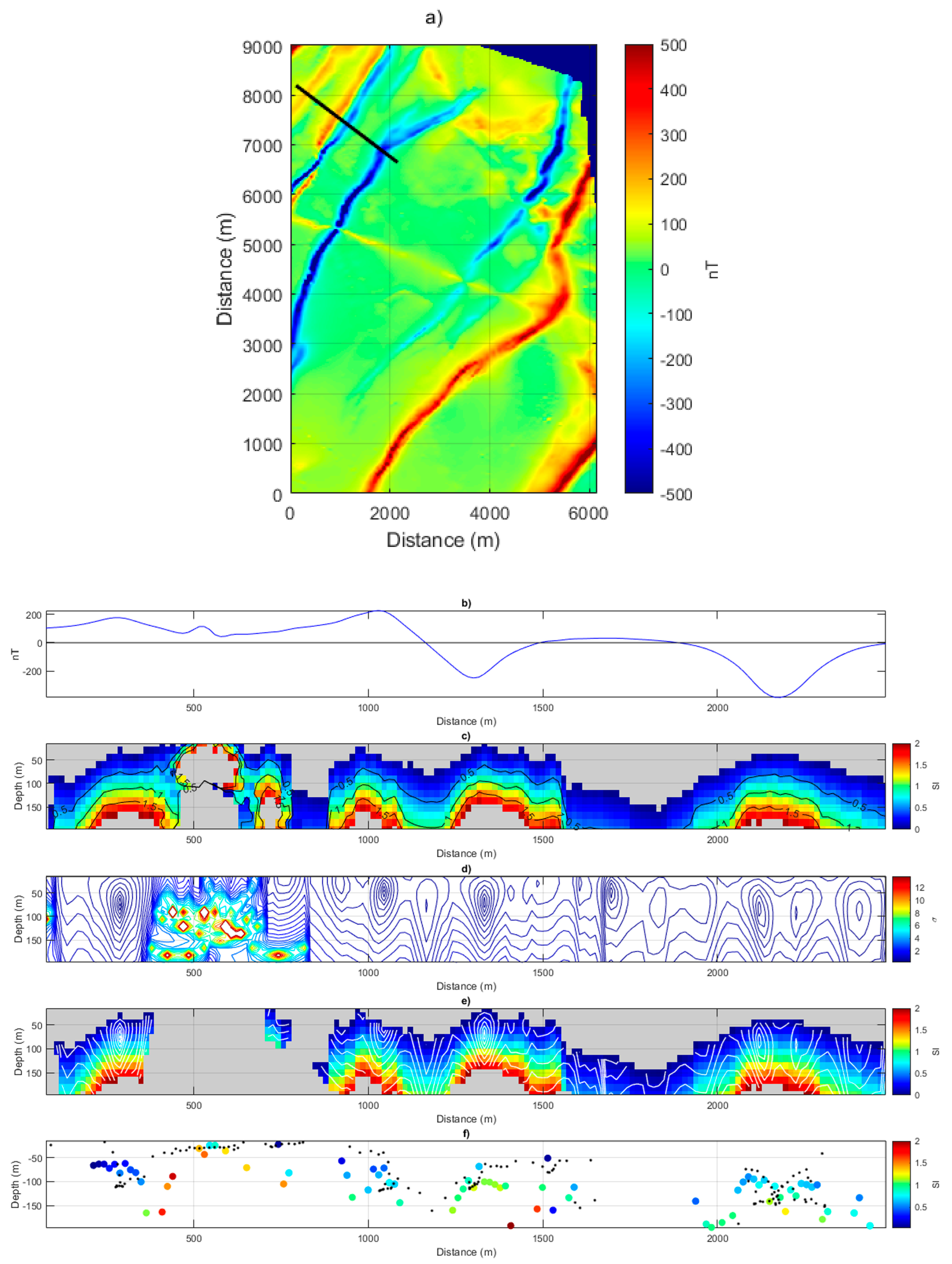
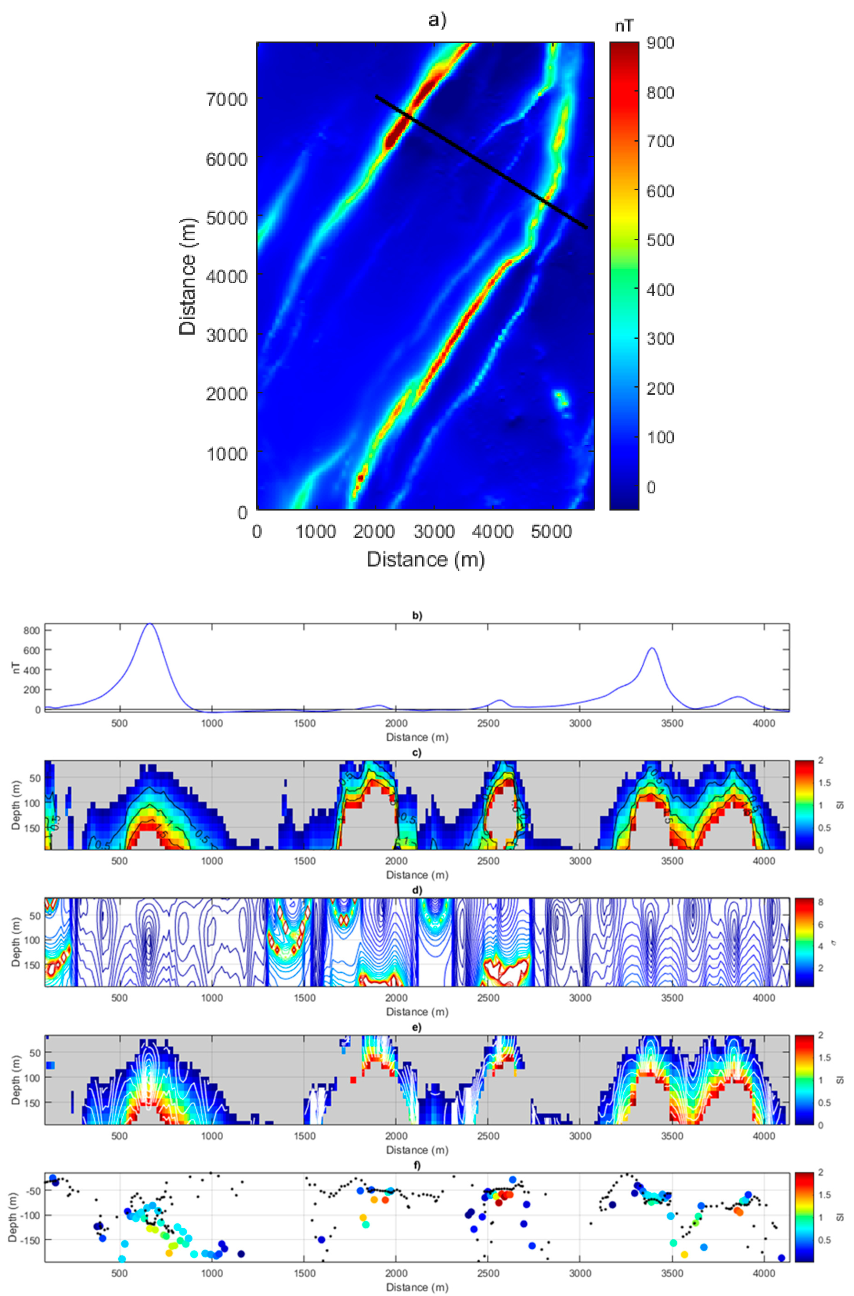
Application to Aeromagnetic Data from the Bushveld Igneous Complex, South Africa

The approximately 2.05 Ga Bushveld Complex is the largest layered igneous intrusion in the world and is a major source of platinum group elements such as chromite, vanadium, and magnetite. It contains mineralised layers that extend for tens of kilometres along strike. It has four main zones and is up to 9 km thick. It has been mined since the early 1900s and contains 70% of the world’s platinum [13]. The platinum mining is affected by the presence of dykes, so an aeromagnetic dataset was collected over a portion of the Critical Zone of the Rustenburg Layered Suite of the eastern Bushveld Complex. The geology of the area is mainly medium- to coarse-grained norite and anorthosite and the economically significant PGE deposits of the UG-2 chromite layer and the Merensky Reef. The NE–SW-trending dolerite dykes are highly fractured and weathered, and palaeomagnetic work has determined them to be of Proterozoic age [14]. The flight height of the aeromagnetic survey was 50.0 m, and the distances to the top of the dykes below this range from 50.0–150.0 m. The magnetic data were gridded to 15 m spacing using the minimum-curvature method.
The application of the interpretation methods described above to a profile extracted from the data leads to interesting results. The plot of the SI is useful in itself, since it gives a clear indication of the depths to the dyke’s upper surface, for any desired value of the SI (the SI = 1 theoretically for dykes and magnetic data, but this relies on a number of assumptions). In addition, its spatial variability both in location and depth gives a measure of its stability. For example, at a distance of 500 m on the profile the indicated SI varies widely within a short distance, and even exceeds the plotted maximum value of 2. This is probably caused by cultural features or other noise. Figure 5c shows the local variation of the SI and it is chaotic in this location. In contrast, the local variation shows clear minima beneath the four main dyke anomalies. The combination of the local variation contours with the image of the SI (Figure 5d) shows indicated distances of 50–100 m and SI values from 0.5–1.0. For comparison Euler deconvolution results (using a fixed SI of 1.0) and source-distance results (using Equation (4), then Equation (5) to obtain the SI) are also shown. The Euler deconvolution solutions have groupings in the dyke locations, but as is characteristic of the method, solutions are also scattered throughout the majority of the subsurface. The source-distance results (which are obtained at each individual point along the profile, and hence are not subject to any horizontal smearing as occurs with methods that use a data window) also show grouping in similar locations, while the indicated SI values are useful in discriminating between valid and invalid solutions (the latter being caused by noise, interference, etc.). However, the variation images have improved horizontal resolution compared to these techniques and are particularly useful when combined with the SI information (Figure 5e).
A second profile was then examined similarly (Figure 6a). There are two main anomalies on the profile, at distances of 600 m and 3400 m. Both resulted in interpreted source depths of about 100 m and SI values close to 1, using clear minima of the variation of the SI as a guide to these parameters (Figure 6c–e). Euler deconvolution results (with SI chosen as 1) gave similar results, but the solutions were not well clustered horizontally and were generally scattered throughout the plot (Figure 6f). The source-distance solutions were better clustered and additionally gave information on the associated SI (from Equation (5)). However, neither of these methods had the horizontal resolution of the variation contours. There are three additional, weaker magnetic anomalies on the profile, at distances of 1900, 2600, and 3800 m. The SI variation contours indicated a depth of about 100 m for the latter, to which the Euler and source-distance methods agreed. The other two anomalies appeared to be shallower, probably outcropping, from all three interpretation approaches.

4. Conclusions

It is well known that platinum mining in the Bushveld Igneous Complex, South Africa is adversely affected by the frequent occurrence of dykes in the area. The recent resurgence in the price of platinum has resulted in renewed geophysical activity in the area to assist mining operations [15]. Re-interpretation of legacy data to extract more information using modern techniques is an inexpensive approach in this regard. New techniques for processing aeromagnetic data have been presented which provide considerable additional information about the magnetic properties of the subsurface, and these were demonstrated using data from an area where dykes are prevalent. Because the orders of the derivatives of the field that the method uses can be finely controlled, factors such as noise and interference are not as serious for the method as is the case for many other methods.

Funding

This research received no external funding.

Data Availability Statement

The Anglo American Corporation should be approached for access to the aeromagnetic data shown in this manuscript.

Acknowledgments

Gordon Chunnett of Anglo Platinum is thanked for providing the data shown in Figure 5 and Figure 6.

Conflicts of Interest

The author declares no conflict of interest.

References

  1. Mpofana, S.; Hloušek, F.; Manzi, M.; Rapetsoa, M.; Buske, F.; Khoza, D. Seismic imaging of the complex geological structures in the southwestern edge of the Western limb, Bushveld Complex through focusing pre-stack depth migration of legacy 2D seismic data. Geophys. Prospect. 2024, 72, 2504–2519. [Google Scholar]
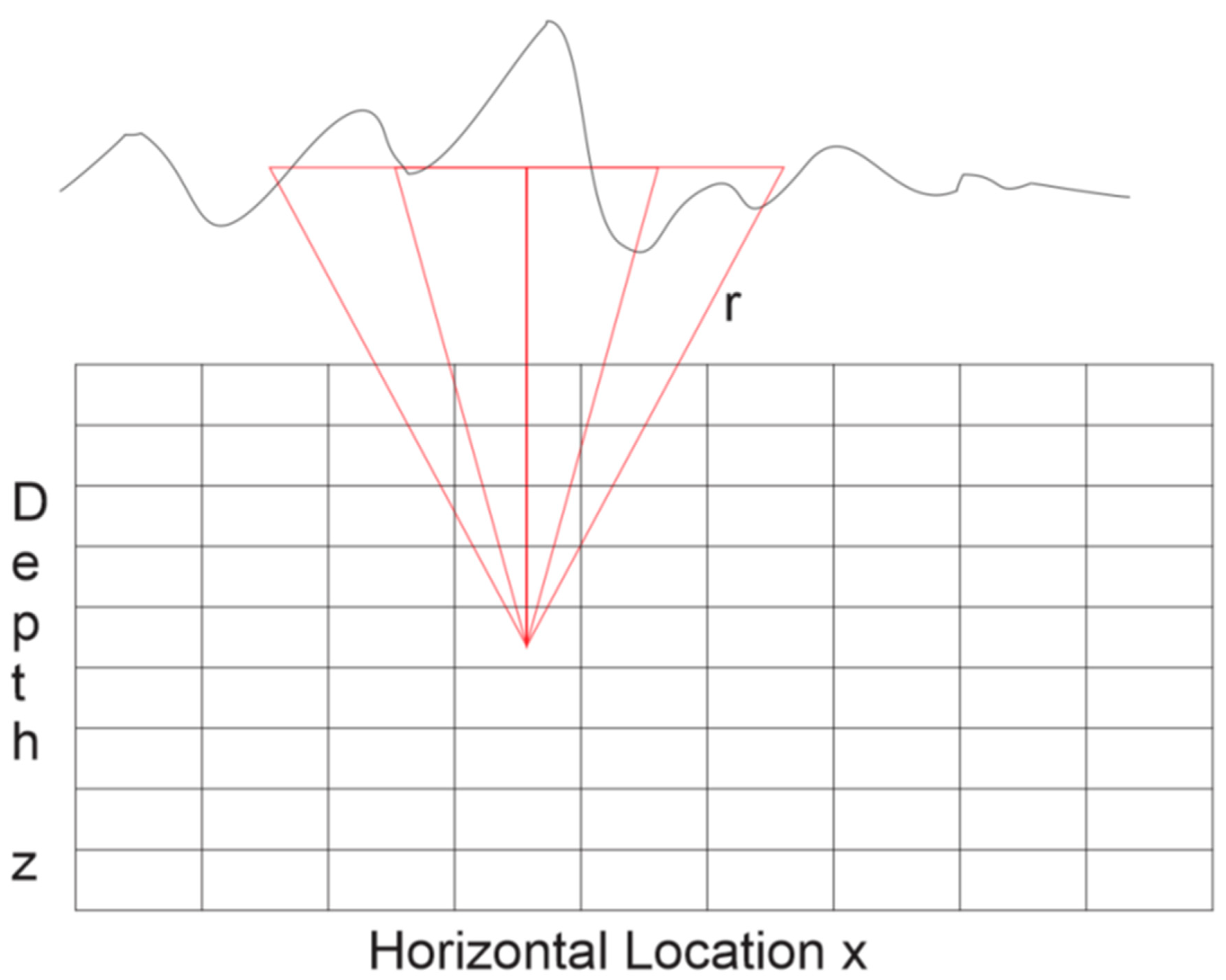
  2. Cooper, G.R.J. Euler Deconvolution in a Radial Coordinate System. Geophys. Prospect. 2014, 62, 1169–1179. [Google Scholar] [CrossRef]
  3. Salem, A.; Williams, S.E.; Fairhead, J.D.; Ravat, D.; Smith, R. Tilt-depth method: A simple depth estimation method using first-order magnetic derivatives. Lead. Edge 2007, 26, 1502–1505. [Google Scholar] [CrossRef]
  4. Huang, L.; Zhang, H.L.; Sekelani, S.; Wu, Z.C. An improved Tilt-Euler deconvolution and its application on a Fe-polymetallic deposit. Ore Geol. Rev. 2019, 114, 103114. [Google Scholar] [CrossRef]
  5. Huang, L.; Zhang, H.L.; Li, C.-F.; Feng, J. Ratio-Euler deconvolution and its applications. Geophys. Prospect. 2022, 70, 1016–1032. [Google Scholar] [CrossRef]
  6. Reid, A.B.; Allsop, J.M.; Granser, H.; Millet, A.J.; Somerton, I.W. Magnetic interpretation in three dimensions using Euler deconvolution. Geophysics 1990, 55, 80–91. [Google Scholar] [CrossRef]
  7. Thompson, D.T. Euldph: A new technique for making computer assisted depth estimates from magnetic data. Geophysics 1982, 47, 31–37. [Google Scholar] [CrossRef]
  8. Salem, A.; Ravat, D.; Smith, R.S.; Ushijima, K. Interpretation of magnetic data using an enhanced local wavenumber (ELW) method. Geophysics 2005, 70, L7–L12. [Google Scholar] [CrossRef]
  9. Cooper, G.R.J. A generalized source-distance semi-automatic interpretation method for potential field data. Geophys. Prospect. 2023, 71, 713–721. [Google Scholar] [CrossRef]
  10. Hsu, S.; Sibuet, J.; Shyu, C. High-resolution detection of geologic boundaries from potential-field anomalies: An enhanced analytic signal technique. Geophysics 1996, 61, 373–386. [Google Scholar] [CrossRef]
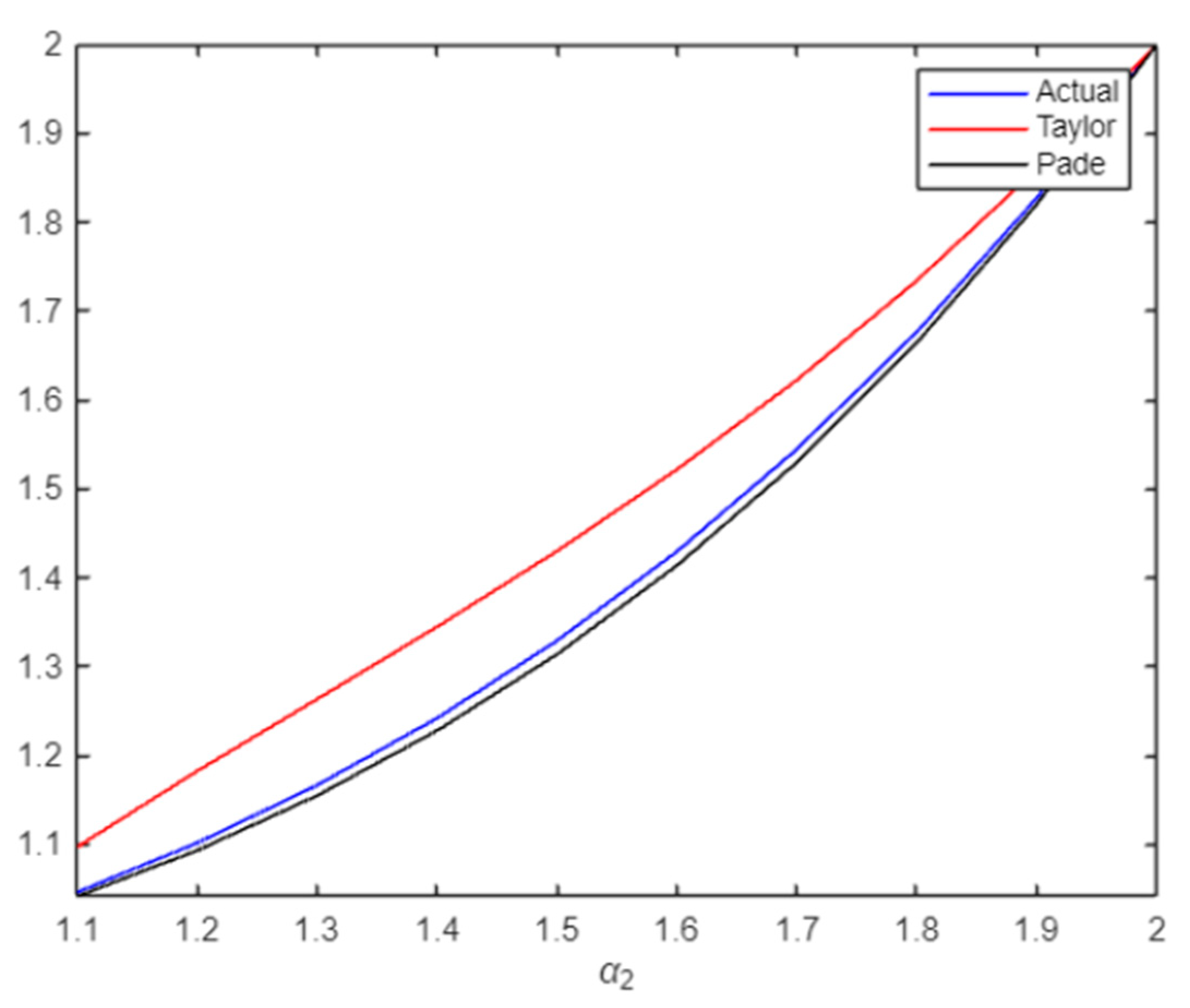
  11. Zhou, W.; Li, J.; Yuan, Y. Downward Continuation of Potential Field Data Based on Chebyshev–Padé Approximation Function. Pure Appl. Geophys. 2018, 175, 275–286. [Google Scholar] [CrossRef]
  12. Pasteka, R.; Richter, F.P.; Karcol, R. and Hajach, M. Regularized derivatives of potential fields and their role in semi-automated interpretation methods. Geophys. Prospect. 2009, 57, 507–516. [Google Scholar] [CrossRef]
  13. Von Gruenewaldt, G.; Sharpe, M.R.; Hatton, C.J. The Bushveld Complex: Introduction and Review. Econ. Geol. 1985, 80, 803–812. [Google Scholar] [CrossRef]
  14. Letts, S.; Torsvik, T.H.; Webb, S.J.; Ashwal, L.D.; Eide, E.A.; Chunnett, G. Palaeomagnetism and 40Ar/39Ar geochronology of mafic dykes from the eastern Bushveld Complex (South Africa). Geophys. J. Int. 2005, 162, 36–48. [Google Scholar] [CrossRef]
  15. Rapetsoa, M.; Manzi, M.; James, I.; Mpofana, S.; Durrheim, R.; Pienaar, M. Innovative Seismic Imaging of the Platinum Deposits, Maseve Mine: Surface and In-Mine. Minerals 2024, 14, 913. [Google Scholar] [CrossRef]
Figure 1. Shows how the subsurface is discretised into a grid, and how the distance from each measurement point in the moving window (in this case five points wide) to each point is calculated.
Minerals 15 00793 g001
Figure 2. Comparison of the relative accuracy of the numerical approximation of Γ(1 + α2)/Γ(1 + α1) for α1 = 1 and 1.1 < α2 < 2. The correct values are plotted in blue, while the Padé expansion approximation is in black and the Taylor expansion is shown in red. The number of terms used in each expansion was the same.
Minerals 15 00793 g002
Figure 3. (a) Profile of magnetic data from the model shown in (be). (b) Median SI obtained from Equation (4) at each location in the subsurface using a window size of 31 points (1500 m). Only values between 0 and 2 are plotted. Values of α1 = 1.7 and α2 = 1.72 were used. (c) Standard deviation σ of SI values obtained at each point using the data values in the moving window. (d) Median SI shown with contours of standard deviation σ overlain. (e) Solutions from Euler deconvolution (black dots) using an SI of 1 and source-distances from Equation (4) are shown. Overlain on the latter are structural indices obtained from Equation (5), with α3 = 1.74.
Minerals 15 00793 g003
Figure 4. (a) Median SI obtained from Equation (4) at each location in the subsurface after uniformly distributed random noise of amplitude of 0.5% of the difference between the data maximum and minimum values was added to the data shown in Figure 3a. Only values between 0 and 2 are plotted. Values of α1 = 1.7 and α2 = 1.72 were used. (b) Standard deviation σ of SI values obtained at each point using the data values in the moving window. (c) Median SI shown with contours of standard deviation σ overlain. (d) Median SI obtained from Equation (4) at each location in the subsurface. Only values between 0 and 2 are plotted. Values of α1 = 0.9 and α2 = 0.92 were used. (e) Standard deviation σ of SI values obtained at each point using the data values in the moving window. (f) Median SI shown with contours of σ overlain.
Minerals 15 00793 g004
Figure 5. (a) Aeromagnetic data over a portion of the the Bushveld Igneous Complex, South Africa. The grid interval is 15.0 m. The black line shows the location of the profile shown in (b) below. (b) Profile of magnetic data from the data shown in Figure 5a. (c) Median SI obtained from Equation (5) at each location in the subsurface using a window size of 15 points (210 m). Only values between 0 and 2 are plotted. Values of α1 = 1.1 and α2 = 1.2 were used. (d) Standard deviation σ of SI values obtained at each point using the data values in the moving window. (e) Median SI shown with contours of standard deviation σ overlain (f) Solutions from Euler deconvolution (black dots) using an SI of 1 and source-distances from Equation (4) are shown. Overlain on the latter are structural indices obtained from Equation (5), with α3 = 1.3.
Minerals 15 00793 g005
Figure 6. (a) Aeromagnetic data over a portion of the the Bushveld Igneous Complex, South Africa. The grid interval is 15.0 m. The black line shows the location of the profile shown in (b) below. (b) Profile of magnetic data from the data shown in (a). (c) Median SI obtained from Equation (4) at each location in the subsurface using a window size of 15 points (210 m). Only values between 0 and 2 are plotted. Values of α1 = 1.2 and α2 = 1.3 were used. (d) Standard deviation σ of SI values obtained at each point using the data values in the moving window. (e) Median SI shown with contours of standard deviation σ overlain. (f) Solutions from Euler deconvolution (black dots) using an SI of 1 and source-distances from Equation (1) are shown. Overlain on the latter are structural indices obtained from Equation (5), with α3 = 1.4.
Minerals 15 00793 g006
Disclaimer/Publisher’s Note: The statements, opinions and data contained in all publications are solely those of the individual author(s) and contributor(s) and not of MDPI and/or the editor(s). MDPI and/or the editor(s) disclaim responsibility for any injury to people or property resulting from any ideas, methods, instructions or products referred to in the content.

