Adaptive Differential Evolution Algorithm for Induced Polarization Parameters in Frequency-Domain Controlled-Source Electromagnetic Data

Abstract

The frequency-domain controlled-source electromagnetic method (CSEM) has been widely used in fields such as oil and gas and mineral resource exploration. In areas with a significant IP response, the CSEM signals will be modified by the IP response of the subsurface. Accurately extracting resistivity and polarization information from CSEM signals may significantly improve the exploration interpretations. In this study, we replaced real resistivity with the Cole–Cole complex resistivity model in a forward simulation of the CSEM to obtain electric field responses that included both induced polarization and electromagnetic effects. Based on this, we used the adaptive differential evolution algorithm to perform a 1-d inversion of these data to extract both the resistivity and IP parameters. Inversion of the electric field responses from representative three-layer geoelectric models, as well as from a more realistic seven-layer model, showed that the inversions were able to effectively recover resistivity and polarization information from the modeled responses, validating our methodology. The electric field response of the real geoelectric model, with 20% random noise added, was then used to simulate actual measured CSEM signals, as well as subjected to multiple inversion tests. The results of these tests continued to accurately reflect the resistivity and polarization information of the model, confirming the applicability and reliability of the algorithm. These results have significant implications for the processing and interpretation of CSEM data when induced polarization effects merit consideration and are expected to promote the use of the CSEM in more fields.

1. Introduction

The CSEM has been widely applied in fields such as oil and gas, metal ore, geothermal, and hydrogeological resource exploration. However, the actual collected CSEM field signals are often the result of combinations of electromagnetic induction and the induced polarization effect. Determining how best to separate these effects during subsequent data processing steps, to obtain resistivity and polarization information regarding the underground geological body being surveyed, is particularly important when processing and interpreting CSEM data. J. Bertine demonstrated the existence of induced polarization effects and analyzed the mechanisms of induced polarization through a series of experiments conducted in 1980 [1]. If a real resistivity model is used instead of a complex one during the forward modeling of the CSEM, the results tend to deviate significantly from the calculated values with the complex resistivities, leading to reduced accuracy [2]. Therefore, researchers have replaced real resistivity with a complex resistivity model that accurately represents induced polarization information to obtain electromagnetic field responses that include both electromagnetic and induced polarization effects. This approach also facilitates accurate analyses of the influence of induced polarization information on CSEMs [3,4,5,6,7,8,9,10,11]. Most work related to extracting polarization information has focused on exploring and verifying the feasibility of methods to extract induced polarization information [12]. Such approaches have been used to analyze polarization anomalies induced by parameter changes in polarization models and the corresponding relationships between model parameters, and both linear and quasilinear inversion methods have been used to quantitatively analyze the galvanic information present in CSEM signals [13,14,15,16,17,18]. However, because linear inversion methods largely depend on initial values that are close to the true model to converge, they are prone to getting trapped in local minima. Fully nonlinear inversion methods therefore provide potential new approaches to handling and interpreting CSEM data that may overcome these challenges.

The differential evolution algorithm, proposed by Storn and Price in 1997 [19], represents a simple and efficient global optimization algorithm with excellent optimization capabilities that has been widely applied in geophysical applications [20,21,22,23]. In this study, we improved the adaptability of control parameter selection in the traditional differential evolution algorithm to adjust the adaptive control parameter, introduced constraints in the objective function to form a minimum structure inversion, and then conducted a one-dimensional adaptive differential evolution inversion study for CSEMs. Our inversion results, based on theoretical responses and field data, indicated that the algorithm has a more robust global search capability and higher inversion accuracy compared to conventional methods and can effectively extract both resistivity and polarization information.

2. Methodology

2.1. One-Dimensional Forward-Modeling Theory of the Controlled-Source Frequency-Domain Electromagnetic Method Considering the Induced Polarization Effect

2.1.1. The Cole–Cole Model

The Cole–Cole model is a complex resistivity model, first proposed by the Cole brothers in 1941, that is used to describe the induced polarization effects present in rocks and ores [24]. In 1978, Pelton et al. concluded that the Cole–Cole model effectively described the complex resistivity characteristics of rocks and ores, based on a large dataset of experimental measurement results from rocks and ores [25]. They therefore applied the Cole–Cole model in geophysical exploration and achieved favorable results. The frequency-domain Cole–Cole model is expressed as follows:

$$\rho \left(\omega \right)={\rho }_0\left\{\mathsf{\eta }\left[1-{\displaystyle \frac{1}{1+{\left(j\omega \tau \right)}^c}}\right]\right\}$$

(1)

where ω = 2πf represents the angular frequency, in rad/s, with f in Hz; $\rho \left(w\right)$ and ${\rho }_0$ represent the complex resistivity of the medium at frequency ω and the zero-frequency resistivity, respectively, both in units of Ω∙m; η represents the polarizability; $\tau$ is the time constant, in second; and $c$ is the frequency-dependent coefficient.

2.1.2. One-Dimensional Forward-Modeling of the Controlled-Source Frequency-Domain Electromagnetic Method with a Finite-Length Source

When a horizontal electric dipole is placed along the x-direction on the ground, Maxwell’s equations can be used, along with a series of derivations, to express the horizontal electric field component $E_x$ as:

$$E_x={\displaystyle \frac{P_E{\mu }_{0}i\omega }{2\pi }}{\int }_0^{\infty }{\displaystyle \frac{\lambda }{\lambda +\raisebox{1ex}{$n_1$}\!\left/ \!\raisebox{-1ex}{$R_1$}\right.}}{J}_0\left(\lambda r\right)d\lambda +{\displaystyle \frac{P_E{\mu }_{0}i\omega }{2\pi r}}(1-2{cos}^2\theta ){\int }_0^{\infty }\left[{\displaystyle \frac{n_1}{k_1^2{R}_1^{*}}}-{\displaystyle \frac{1}{\lambda +\raisebox{1ex}{$n_1$}\!\left/ \!\raisebox{-1ex}{$R_1$}\right.}}\right]J_1\left(\lambda r\right)d\lambda +{\displaystyle \frac{P_E{\mu }_{0}i\omega }{2\pi r}}{cos}^2\theta {\int }_0^{\infty }\left[{\displaystyle \frac{n_1}{k_1^2{R}_1^{*}}}-{\displaystyle \frac{1}{\lambda +\raisebox{1ex}{$n_1$}\!\left/ \!\raisebox{-1ex}{$R_1$}\right.}}\right]\lambda J_0\left(\lambda r\right)d\lambda$$

(2)

where $E_x$ is the horizontal electric field component in the direction of the source, in $\mathrm{V}/\mathrm{m}$; $P_E$ is the electric dipole moment, in Amperes⋅meters; $P_E=Idl$, where $I$ is the supply current, in Amperes, and $dl$ is the length of the electric dipole source; ${\mu }_0$ is the permeability of vacuum; $i$ is the imaginary unit (√−1); $\omega$ is the angular frequency; $\lambda$ is the integration variable; $u_j=\sqrt{{\lambda }^2+{k_j}^2}$, where ${k_j}^2=-i\omega u_0{\sigma }_j$ and $k_j$ is the complex wave number of the j-th layer; $\mathsf{\theta }$ is the angle between the direction of the dipole source and the vector from the source’s midpoint to the receiver; r is the source–receiver distance; $j=1,2,\cdots ,N$, where $N$ is the number of electrical layers; and $J_1\left(\lambda r\right)$ and $J_0\left(\lambda r\right)$ are the first-order and zero-order Bessel functions of $\lambda r$, respectively. For an $N$-layer stratified Earth medium, which consists of $N$ − 1 layers of finite thickness covering the upper half-space, $R_1$ and $R_1^{*}$ represent two functions that relate the electrical conductivity of the upper half-space to the conductivity of the first layer. These functions depend on the conductivities and thicknesses of the $N$ − 1 layers, as well as the conductivity of the upper half-space. They can be expressed as:

$$R_1=\mathrm{c}\mathrm{t}\mathrm{h}\left[u_1{h}_1+arcth{\displaystyle \frac{u_1}{u_2}}\times \mathrm{c}\mathrm{t}\mathrm{h}(u_2{h}_2+\cdots +arcth{\displaystyle \frac{u_{N-1}}{u_N}})\right]$$

(3)

$$R_1^{*}=\mathrm{c}\mathrm{t}\mathrm{h}\left[u_1{h}_1+arcth{\displaystyle \frac{u_1{\rho }_1}{u_2{\rho }_2}}\times \mathrm{c}\mathrm{t}\mathrm{h}(u_2{h}_2+\cdots +arcth{\displaystyle \frac{u_{N-1}{\rho }_{N-1}}{u_N{\rho }_N}})\right]$$

(4)

In real-world exploration cases, the transmitting source is often not considered an electric dipole but rather a finite-length source or a dipole source. Based on previous related works, we used the Gaussian integration method to solve the electromagnetic response equation for finite-length sources and thus obtain the electric field response of the finite-length source [9,26]. By replacing the real resistivity in Equation (2) with Equation (1), the horizontal electric field response of the CSEM, including the induced polarization information, can be obtained [4,5].

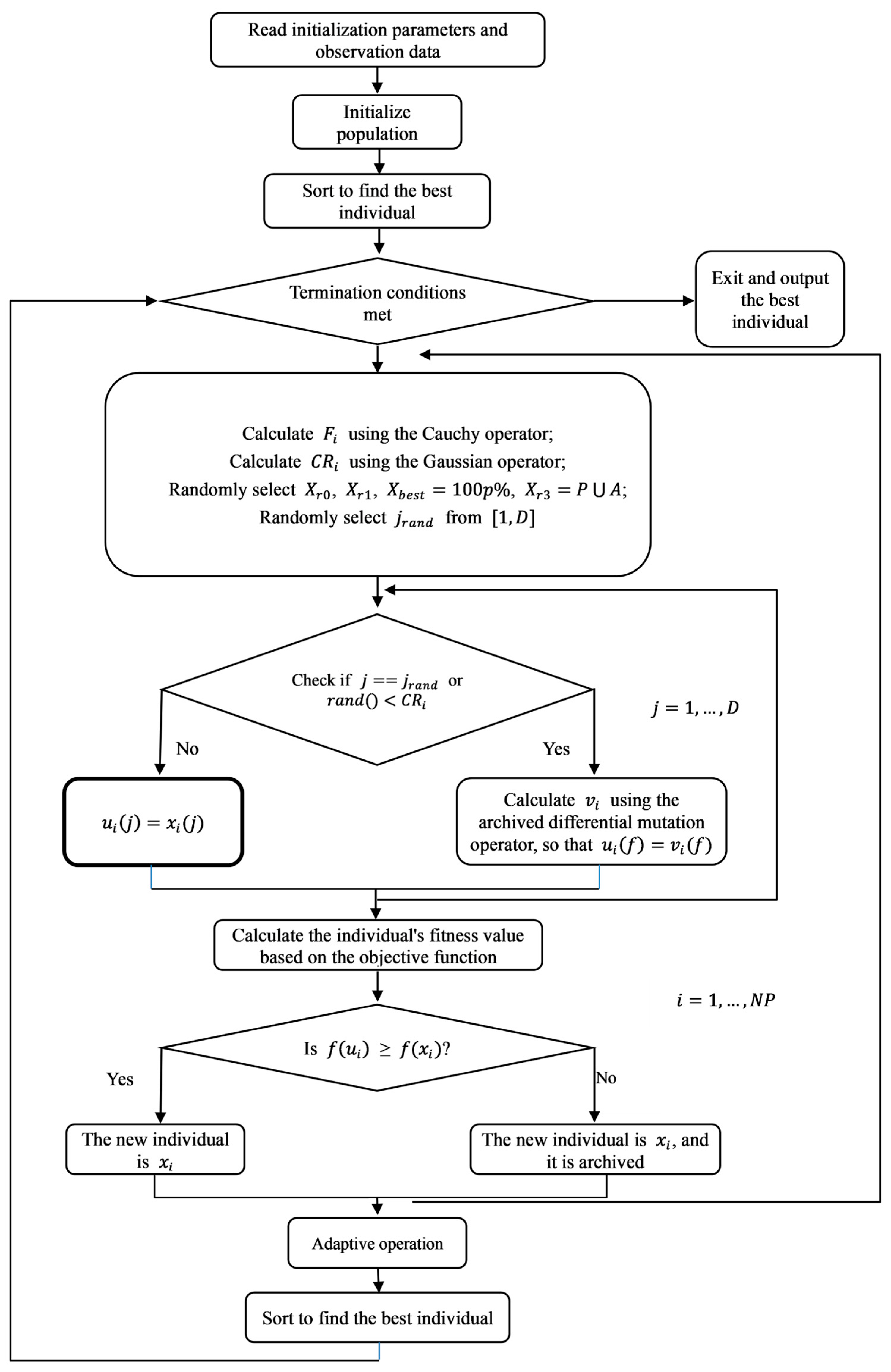
2.2. Adaptive Differential Evolution Algorithm

The joint-mutation and adaptive differential evolution algorithm is a derivative of the differential evolution algorithm proposed by Zhang et al. in 2009 [27]. It primarily addresses the issue of premature convergence in differential evolution algorithms because of improper control parameter settings. The algorithm adapts by using information from successfully evolved individuals during the evolution process and uses Cauchy and Gaussian distributions for adaptive adjustment. In this study, we enhanced the mutation strategy and control parameters in the adaptive differential evolution algorithm to effectively extract resistivity and polarization information from the CSEM. The resultant adaptive differential evolution algorithm consists of population initialization followed by mutation, crossover, and selection operations.

(1) Population Initialization: Based on the population size, the initial population is established by randomly generating NP individuals with N-dimensional model parameters within the boundaries of the model’s parameters. The current iteration number is 1, and the maximum iteration number is G.

(2) Mutation Operation: The mutation strategy directly affects the algorithm’s search capability and convergence performance. The differential strategy selected for this study is an improved DE/current-to-pbest/1 strategy first proposed by Zhang et al., which combines information from the current individual, the best individual, and a random individual [27]. Its goal is to balance global search and local exploitation capabilities, and is expressed as follows:

$$v_{i,j}=X_{i,g}+F_i·\left(X_{best,g}^P-X_{i,g}\right)+F_i·(X_{r1,g}-{\tilde{X}}_{r2,g})$$

(5)

where $X_{i,g}$, $X_{r1,g}$, and $X_{r2,g}$ represent the individuals randomly selected from the current population P, while $X_{best,g}^p$ is the best individual randomly selected from the top 100 p% of individuals in the current population P, where p ∈ (0, 1].

For each individual in the current generation g, the corresponding scaling factor F_i can be generated using a Cauchy distribution:

$$\left\{\begin{array}{l}{F}_i=Cauchy({\mu }_F,\sigma )\\ {\mu }_F=(1-c)·{\mu }_F+c·mea{n}_L(S_F)\end{array}\right.$$

(6)

where Cauchy (•) represents the Cauchy distribution random number generator; ${\mu }_F$ represents the location parameter; σ is the scale parameter; S_F represents the scaling factors F_i of all of the individuals that successfully underwent mutation within the current generation g, with a total of $N_{S_F}$; c is a constant in the range [0, 1]; and ${mean}_L\left(·\right)$ represents the Lehmer mean. The latter is expressed by Equation (7):

$$mea{n}_L={\displaystyle \frac{{\displaystyle {\sum }_{i=1}^{N_{S_F}}{F}_i^2}}{{\displaystyle {\sum }_{i=1}^{N_{S_F}}{F}_i}}}$$

(7)

where ${\mu }_F$ is typically initialized to 0.5, updated according to Equation (6), and then used for the mutation operation in the next generation, and F_i must satisfy the following condition:

$$F_i=\left\{\begin{array}{ll}1& if (F_i>1)\\ Cauchy({\mu }_F,\sigma )& if (F_i=<0)\end{array}\right.$$

(8)

(3) Crossover Operation: A binomial crossover operator is used to combine the mutated vector v_i,j produced by the mutation operator with the parent vector X_i,j, resulting in a new individual u_i,g = (u_i,1,g, u_i,2,g,…, u_i,D,g).

$$u_{i,j,g}=\left\{\begin{array}{ll}{v}_{i,j,g}& if (rand(0,1)<C{R}_i or j=j_{rand})\\ x_{i,j,g}& else\end{array}\right.$$

(9)

where rand (a, b) is a uniform random number in the range [a, b], with each j and each i independently generating random numbers, and j_rand = randint (1, D) is a random integer selected from the range 1 to D. For each individual i, a new random number must be generated. The crossover probability ${CR}_i$ ∈ [0, 1] determines the probability of crossover, with higher values indicating a higher likelihood. ${CR}_i$ generally corresponds to the average portion of the vector component inherited from the mutation vector.

In each iteration, each individual Xi has an associated crossover probability, ${CR}_i$, that can be randomly generated according to a normal distribution:

$$\left\{\begin{array}{l}C{R}_i=Gaussian({\mu }_{CR},\delta )\\ {\mu }_{CR}=(1-c)·{\mu }_{CR}+c·mea{n}_A(S_{CR})\end{array}\right.$$

(10)

where Gaussian (•) represents the normal distribution random number generator; ${\mu }_{CR}$ is the mean; δ represents the standard deviation; $S_{CR}$ represents the crossover probabilities, ${CR}_i$, of all of the individuals that successfully underwent crossover within the current generation g; c is a constant within the range [0, 1]; ${mean}_A\left(·\right)$ is the commonly used arithmetic mean function that is used to calculate the average crossover probability of the successful individuals in the current population; ${\mu }_{CR}$ is typically initialized to 0.5 before being updated according to Equations (10) and subsequently being used for the crossover operation in the next generation; δ is the user-defined input; and ${CR}_i$ must lie within the range [0, 1]. If the latter falls outside of that range, a truncation method is applied to constrain it.

(4) Selection Operation: The differential evolution algorithm adopts the “survival of the fittest” concept to select superior individuals in a self-serving manner, thus ensuring that the algorithm constantly moves toward the global optimum. This operation is performed on the individuals within the population as described in Equation (11):

$$x_i^{t+1}=\left\{\begin{array}{c}{u}_i^{t+1}, f\left(u_i^{t+1}\right)<f\left(x_i^t\right)\\ x_i^t,else\end{array}\right.$$

(11)

where f () is the objective function, operating under the assumption that the problem is one of minimization optimization. Steps (2) to (4) are repeated until the number of iterations reaches the maximum value $G$.

3. Inversion of the Controlled-Source Electromagnetic Method Considering the Induced Polarization Effect

3.1. Objective Function Construction

Our analysis of the response of the CSEM that considers induced polarization information revealed that, in a layered model with polarized media, the horizontal electric field component $E_x$ is the most sensitive to the induced polarization effect [6,15,16]. Therefore, we constructed the objective function $f_d\left(m\right)$ by selecting the error vector between the observed data and the forward-modeled horizontal electric field component $E_x$:

$$f_d\left(m\right)={\left(d-d_f\right)}^T(d-d_f)$$

(12)

where m is the model parameter vector; $d$ is the one-dimensional observed data vector, with a dimension equal to the number of frequency points; $d_f$ is the one-dimensional forward-modeled data vector of the CSEM; and $d_f=G(m,\tau ,c,h,\rho )$, where $G(·)$ is the forward-modeling operator for the controlled-source method.

3.2. Introduction of Minimum Structure

Non-uniqueness is the primary challenge in quantitative geophysical inversion. Inversion of the CSEM with limited observed data is non-unique, meaning that some different models can accurately describe the data. However, if accurately fitting the data is the only consideration, overly complex models may be inverted, or unnecessary structures that cannot be resolved by the data may be introduced, causing inversion instability that creates other difficulties during later interpretation. In this study, we introduced constraints into the objective function to form a minimum structure inversion. Thus, Equation (12) was updated to form the new objective function $f\left(m\right)$:

$$f\left(m\right)=f_d\left(m\right)+\lambda f_m\left(m\right)$$

(13)

where $f\left(m\right)$ is the total objective function, $f_m\left(m\right)$ is the objective function of the model’s constraint, and λ is the regularization factor. The constraint function $f_m\left(m\right)$ can be expressed as:

$$f_m\left(m\right)={\left(Rm\right)}^T\left(Rm\right)$$

(14)

where R is the rough matrix. Equation (13) can then be rewritten as:

$$f_m\left(m\right)=\sum _{i=2}^n{(m_i-m_{i-1})}^2$$

(15)

where n is the number of layers in the earth. For $\lambda$, the regularization factor can be written as [28,29]:

$${\lambda }^k={\displaystyle \frac{f_d^{k-1}\left(m\right)}{f_d^{k-1}\left(m\right)+f_m^{k-1}\left(m\right)}}$$

(16)

where k represents the current iteration number. In the adaptive differential evolution inversion algorithm’s selection operation, individuals are compared based on their $f\left(m\right)$ values, where only new individuals who have fitness values smaller than those of their parents proceed to the next round of evolutionary operations. During the inversion process, the root mean square relative error in Equation (17) is used to measure the performance of the inversion algorithm, according to the formula:

$$RMS=\sqrt{{\displaystyle \frac{1}{N}}\sum _{i=1}^N{\left({\displaystyle \frac{F_{obsi}-F_{mi}}{F_{obsi}}}\right)}^2}\times 100\%$$

(17)

where N represents the number of time points, $F_{obsi}$ is the measured electric field response at the i-th time point, $F_{mi}$ denotes the electric field response calculated by the inversion model at the i-th time point, and RMS represents the root mean square relative error. A smaller RMS value therefore indicates a smaller difference between the measured and predicted values. The inversion flowchart is shown in Figure 1.

4. Theoretical Model Validation

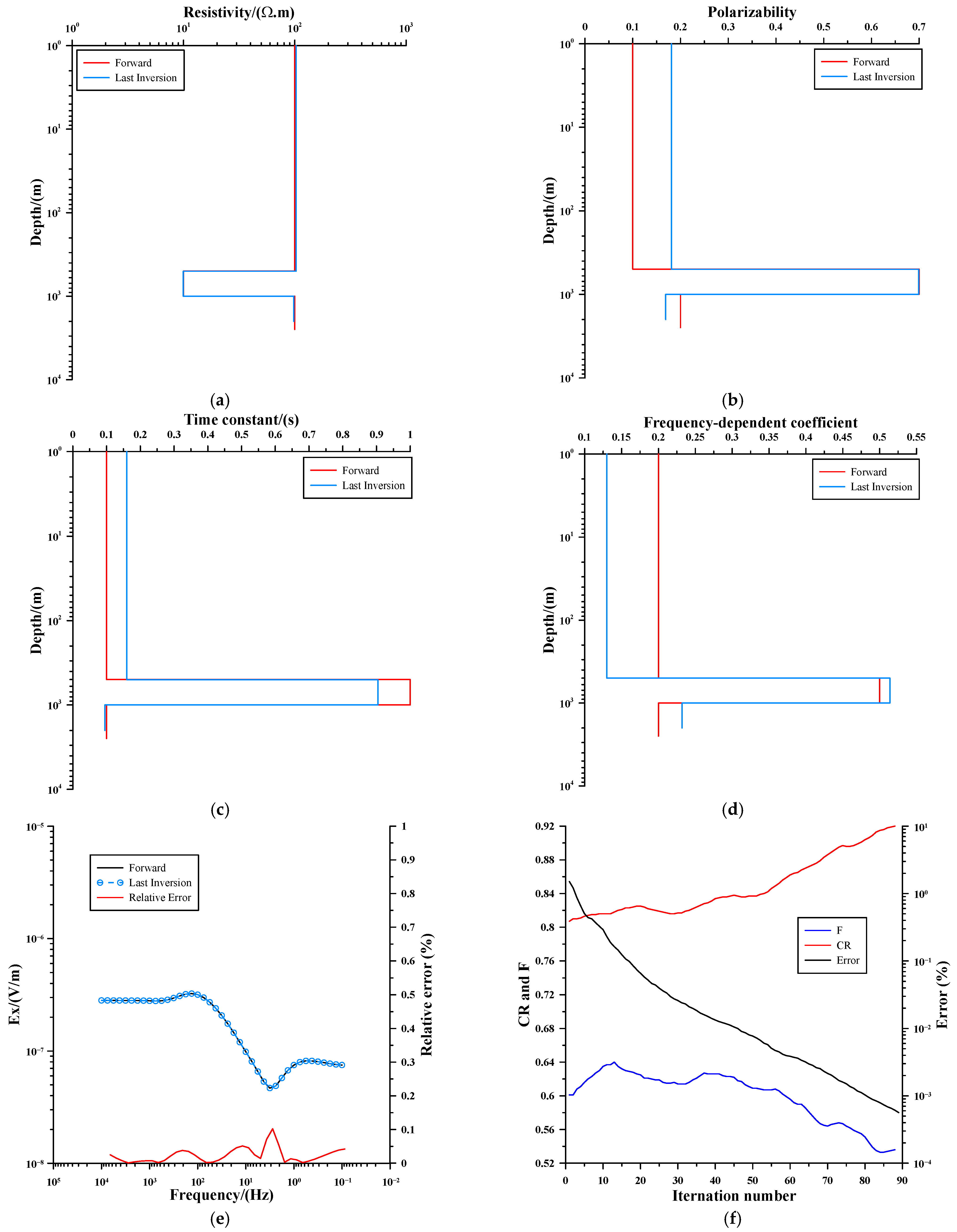
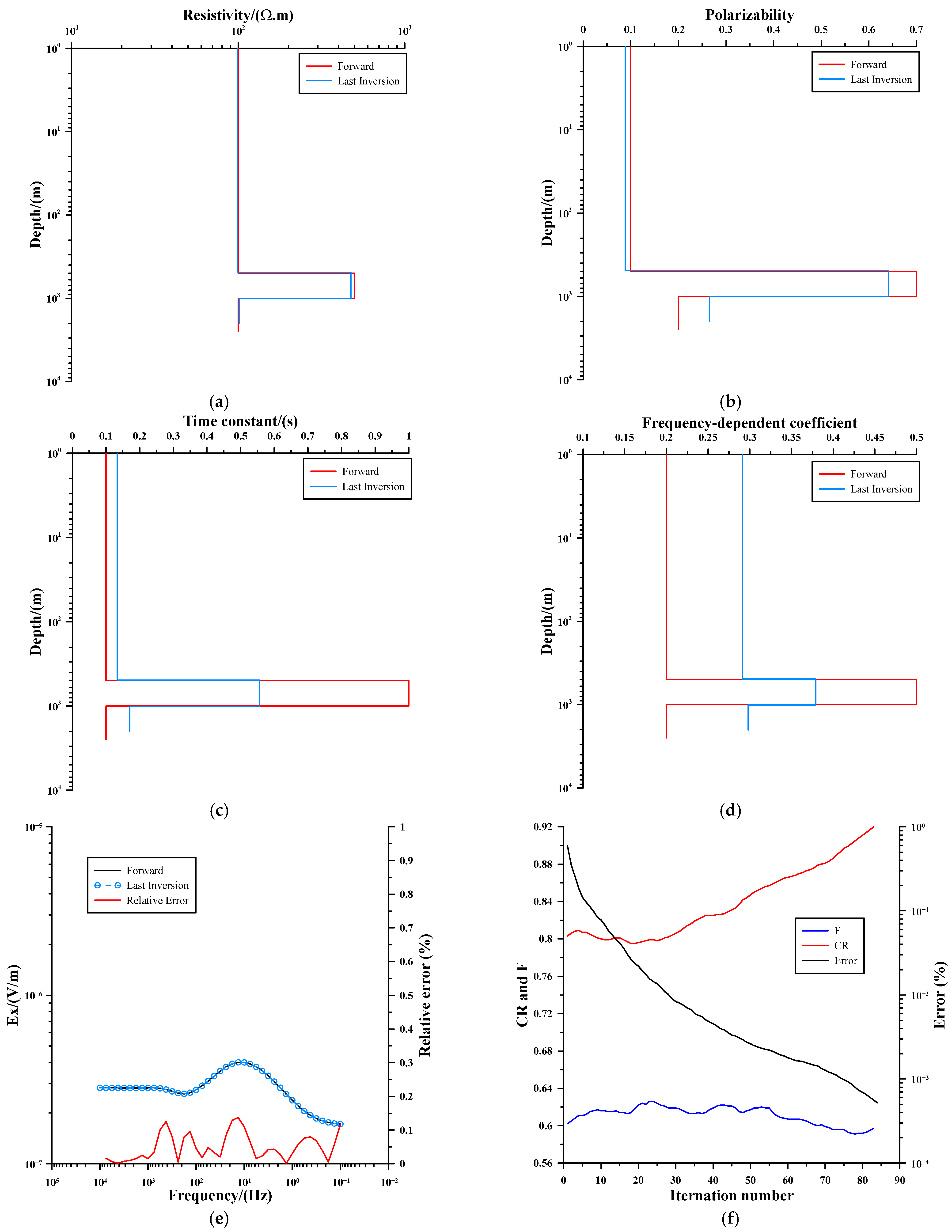
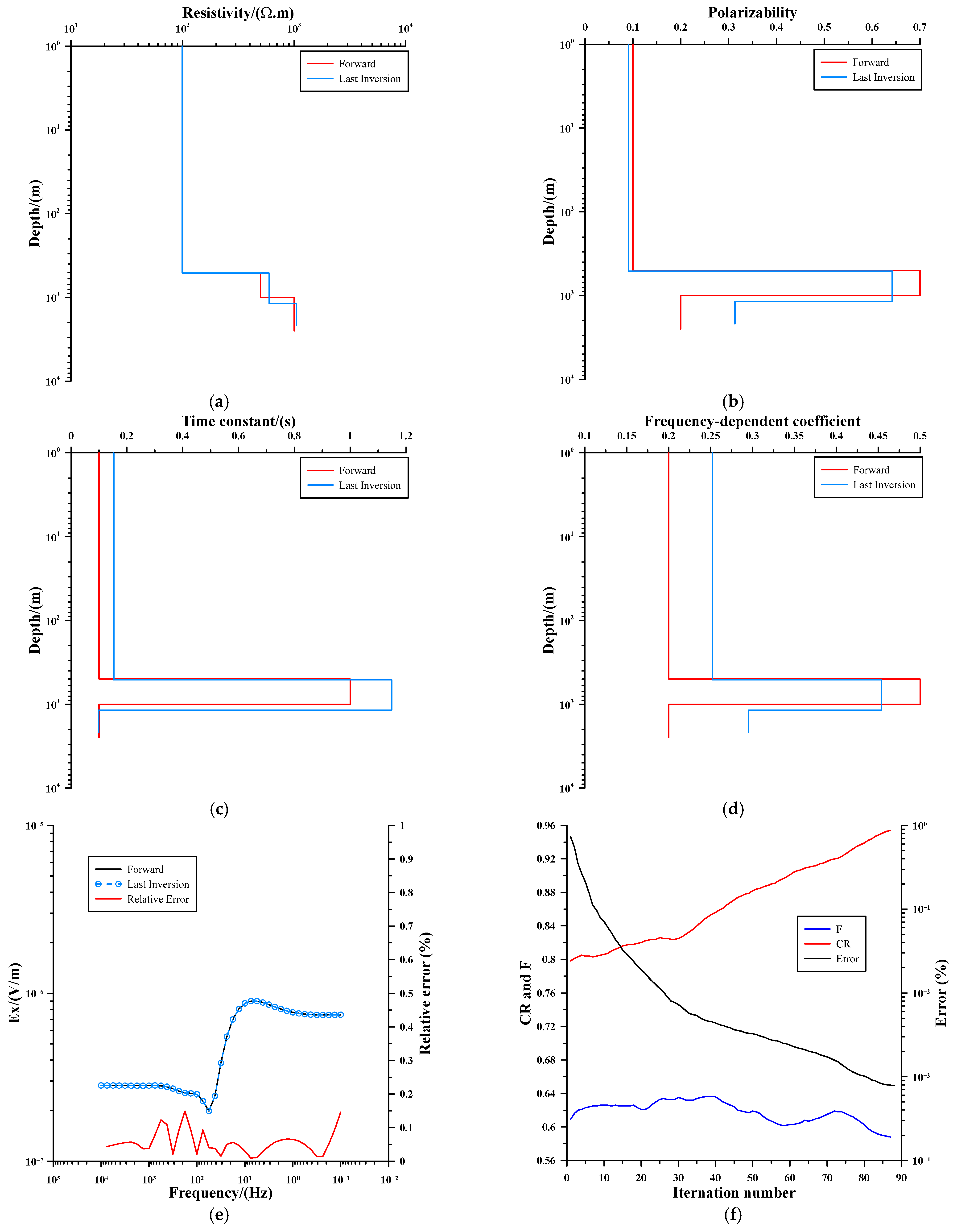
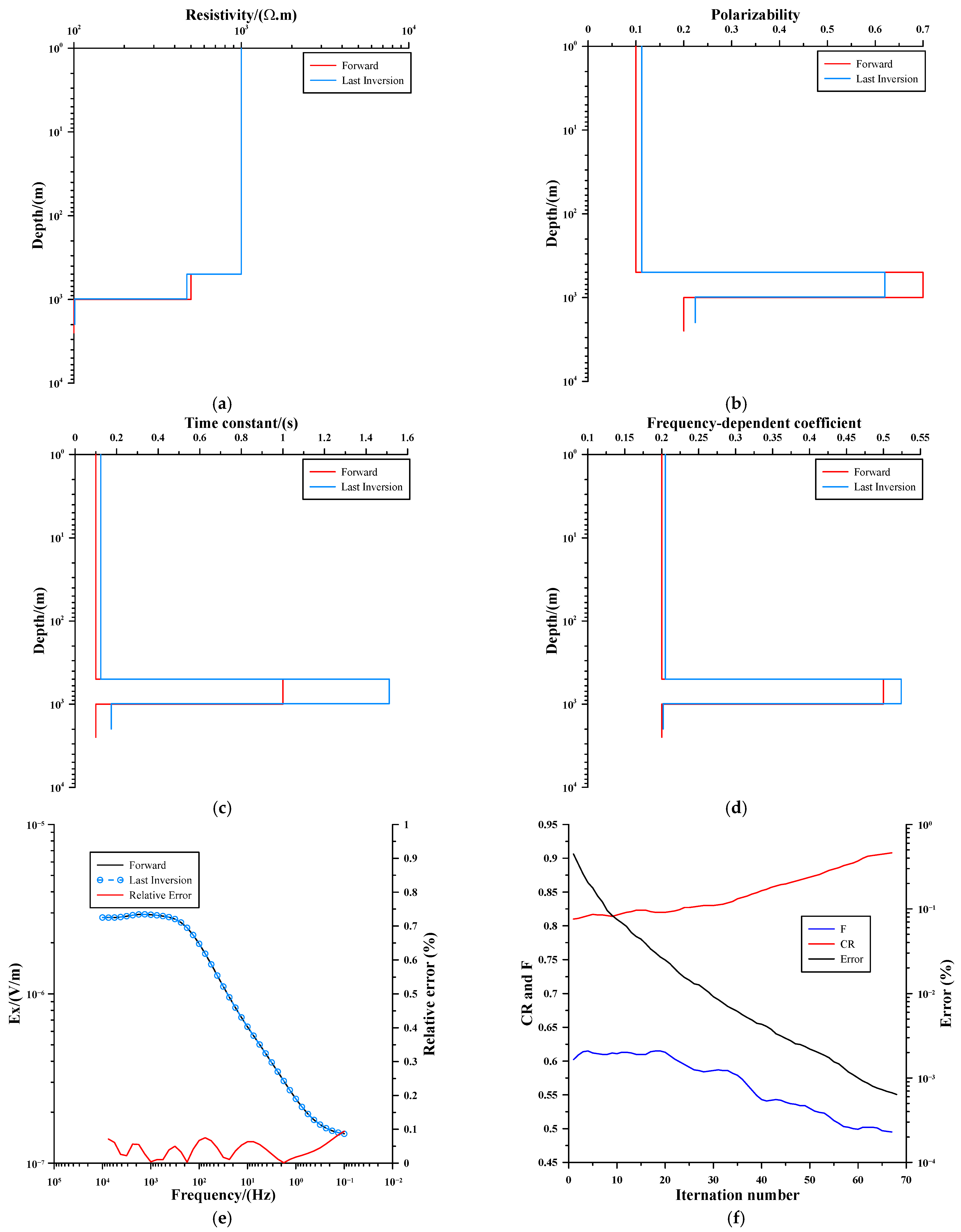
4.1. Representative Three-Layer Geoelectric Model

The theoretical inversion results for a representative three-layer geoelectric model were used to verify the reliability of the algorithm we developed in this study. In the forward calculation, the length of the transmitting source was 2000 m, the coordinates of the receiver measurement points were (100, 6000), and the calculation frequency range was between 0.1 and 10,000 Hz. The geoelectric parameters of the model are shown in

Table 1. Parameters for representative three-layer polarized medium geoelectric models.

Type	Resistivity (Ω·m)	Polarizability	Frequency-Dependent Coefficient	Time Constant (s)	Layer Thickness (m)
H	100/10/100	0.1/0.7/0.2	0.2/0.5/0.2	0.1/1/0.1	500/500/∞
K	100/500/100	0.1/0.7/0.2	0.2/0.5/0.2	0.1/1/0.1	500/500/∞
A	100/500/1000	0.1/0.7/0.2	0.2/0.5/0.2	0.1/1/0.1	500/500/∞
Q	1000/500/100	0.1/0.7/0.2	0.2/0.5/0.2	0.1/1/0.1	500/500/∞

. During the inversion process, the basic parameters of the adaptive differential evolution were set as follows: population size NP = 60, parameters $F$ and $CR$ obtained adaptively, regularization parameter $\lambda =0.5$, and initial ${\mu }_{CR}$ and ${\mu }_F$ values of 0.8 and 0.6, respectively.

Figure 2, Figure 3, Figure 4 and Figure 5 present the theoretical inversion results for the representative three-layer geoelectric models. In each figure, panel (a) shows the inversion result of resistivity; (b) shows the inversion result of polarization; (c) shows the inversion result of the time constant; (d) shows the inversion result of the frequency-related coefficient; (e) shows the fitting of the frequency-domain Ex data and the fitting error at each frequency; and (f) shows the values of ${\mu }_{CR}$, ${\mu }_F$, and the mean fitting error at each iteration. The blue solid line represents the inversion result of the best individual from the final iteration. The final inversion result reveals that the inversion result for resistivity accurately reflects the changes in resistivity that occur with depth. The polarization parameters also accurately reflect the values of the theoretical parameters and describe the trend of how the polarization parameters vary with depth (i.e., low–high–low), indicating the presence of high-polarization anomaly bodies. As shown in panels (e) and (f) of Figure 2, Figure 3, Figure 4 and Figure 5, the inverted electric field data from the model show a perfect match with the theoretical observed data, the relative fitting error at each frequency point is less than 0.2%, and the average fitting error across all frequencies is below 0.1%. The error curve decreases as the inversion progresses, indicating that the differential evolution inversion algorithm can be used to find the optimal solution even in this range. The ${\mu }_{CR}$ curve gradually increases with the number of iterations—indicating that the probability of genetic modifications in individuals increases during the later stages of inversion. This indirectly suggests that the polarization parameters are highly interdependent with other parameters in the model (e.g., the geoelectric ones). Thus, we recommend setting ${\mu }_{CR}$ to a larger value during inversion. Concurrently, the ${\mu }_F$ curve shows a general trend of first increasing, before decreasing later on. During the early stages of inversion, reducing F (the search step size) helps the algorithm quickly converge to a local or global optimum. Conversely, increasing F during the later stages increases the possibility of escaping the local optimum and the likelihood of finding the global optimum, thus improving the stability of the inversion algorithm.

The inversion results for the electrical parameters are generally more accurate than those for the polarization parameters. From the fitting results of each model, although the curve fits well and the algorithm can effectively invert the distribution of the underground medium, some discrepancies between the model parameters and the theoretical model nevertheless remain—most likely attributable to non-uniqueness. Based on the changes observed in the ${\mu }_{CR}$ and ${\mu }_F$ curves, as well as the mean fitting errors, it can be concluded that the algorithm can accurately find the optimal solution even during the later stages of inversion.

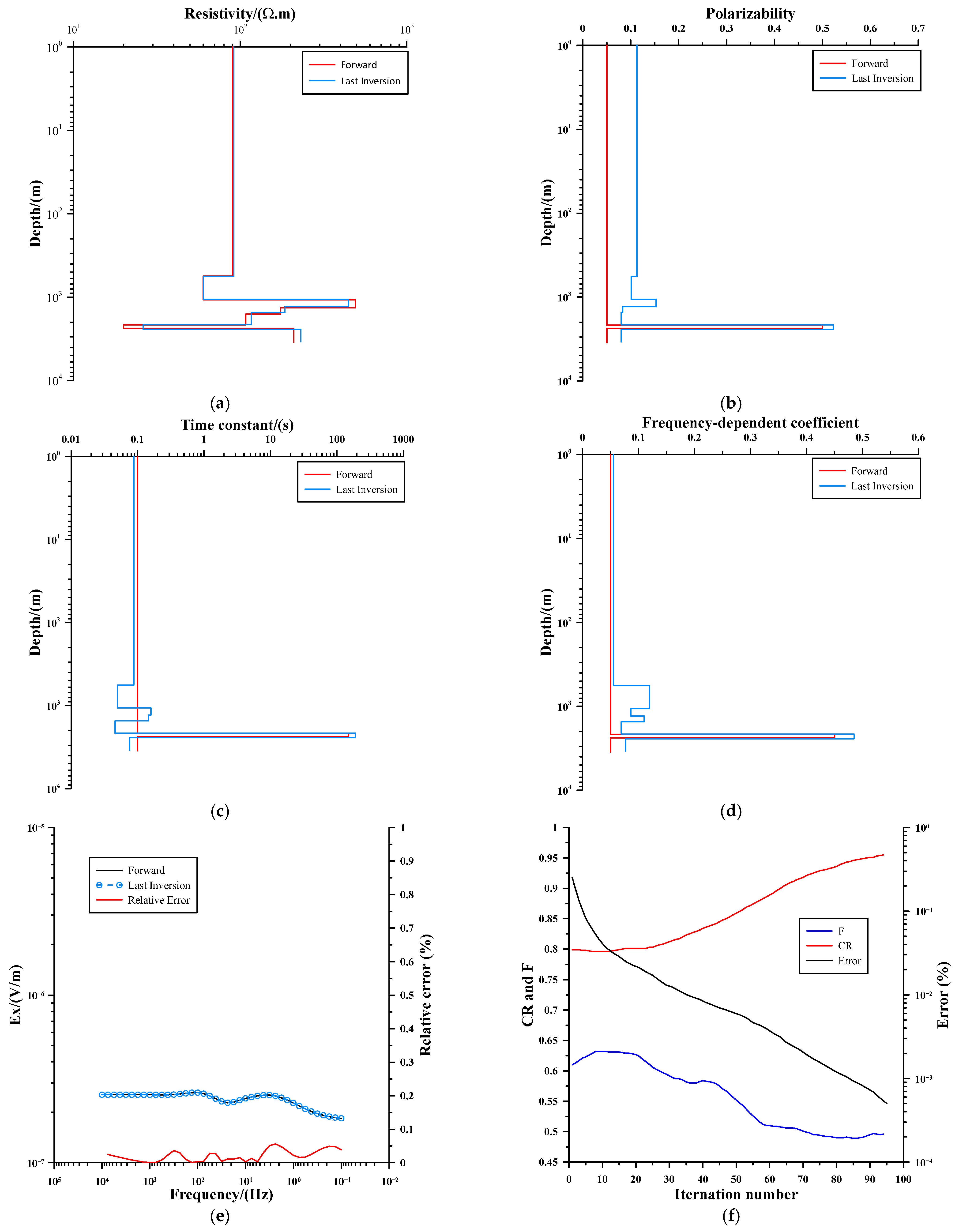
4.2. Real-World Geoelectric Model

4.2.1. Inversion of Theoretical Model Data

To further test the effectiveness of this algorithm in practical applications, we used a seven-layer model for forward calculations, as shown in

Table 2. Simulation parameters for a real geological formation.

Layer No.	Resistivity (Ω·m)	Polarizability	Frequency-Dependent Coefficient	Time Constant (s)	Layer Thickness (m)
1	90	0.05	0.05	0.1	560
2	60	0.05	0.05	0.1	520
3	490	0.05	0.05	0.1	270
4	175	0.05	0.05	0.1	250
5	108	0.05	0.05	0.1	560
6	20	0.5	0.45	150	210
7	210	0.05	0.05	0.1	----

; the other selected simulation parameters were consistent with those used for the representative theoretical three-layer model. During the inversion process, the population size was set to NP = 140 (with 34 model parameters), the parameters F and CR were obtained adaptively, the regularization parameter was $\lambda =0.5$, the initial values of ${\mu }_{CR}$ and ${\mu }_F$ were 0.8 and 0.6, respectively, and c and p were both set to 0.1.

Figure 6 shows the inversion results of the model applied to the real-world geoelectric model. Both the resistivity and polarization information accurately reflected the model’s actual parameters, and the observed data aligned well with the predicted ones. Panel (a) shows that the inversion of resistivity and layer thickness aligned well with the theoretical model. Panels (b), (c), and (d) show that the inversion results for polarizability, the time constant, and the frequency-dependent coefficient (respectively) also corresponded well with the theoretical model. This indicates a strong ability to correctly resolve anomalies (i.e., formations) with low resistance and high polarization. Panel (e) shows that the theoretical data match the predicted ones closely. And the relative fitting error at each frequency point is less than 0.1%. The error curve shows a decreasing trend in panel (f), indicating that the algorithm can determine the optimal solution. The ${\mu }_{CR}$ curve gradually increases with the number of iterations, indicating that the model can still be modified even during the later stages of the inversion process. The ${\mu }_F$ curve exhibits a generally increasing trend at first, followed by a decreasing one, meaning that the algorithm has a higher probability of finding the global optimum during the later stages of inversion, where the stability of its inversion component improves. These data demonstrate that the algorithm shows comparable feasibility for use with real-world data to what was determined earlier in the representative theoretical model.

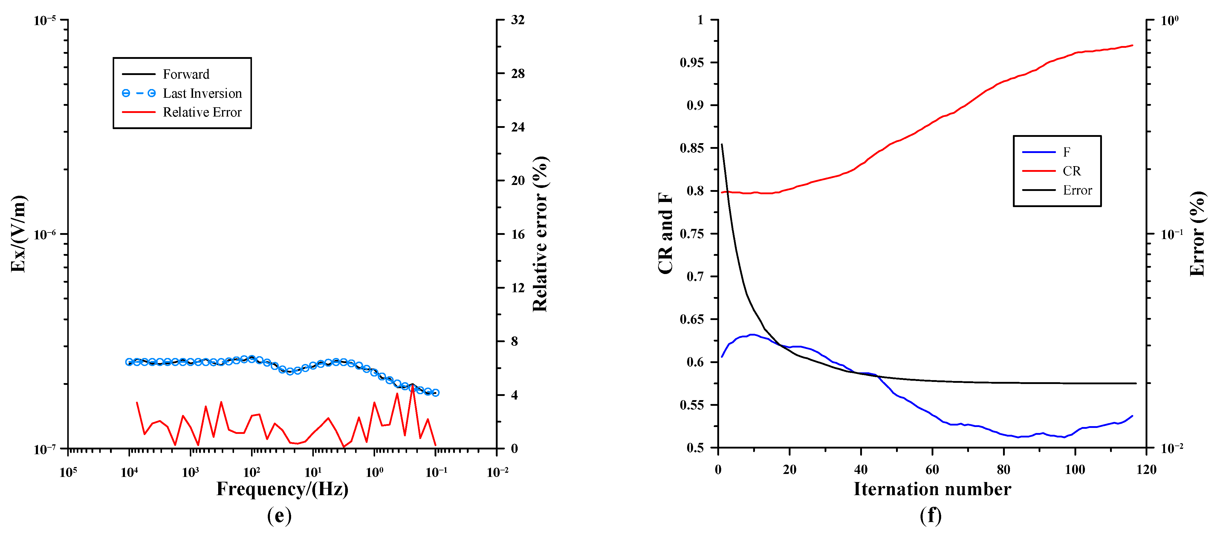
4.2.2. Inversion of Noisy Data

To further test the applicability and stability of the algorithm regarding real-world data, 20% random noise was added to the real-world forward-modeling data to simulate practical field measurement data. During the inversion process, all the parameters for this test were identical to the ones used in the case without noise. Figure 7 shows the inversion results for this experiment. Panels (a), (b), (c), and (d) demonstrate that resistivity, polarizability, the time constant, and the frequency-dependent coefficient (respectively) all correspond well with the values obtained for the theoretical model. However, a certain discrepancy in the calculated depth was noted, owing to the effects of the introduced noise. Thus, depth information should ideally be calibrated using known data from previously drilled wells when the inversion process is applied to real-world data. Panels (e) and (f) in the figure show that the $E_x$ response curve with the added noise aligned well with the predicted Ex response curve, with the average fitting error only rising to 2%. The inversion iteration error also decreased steadily as the number of iterations increased, indicating that the algorithm exhibits favorable applicability to noisy real-world data as well and that its inversion is able to quickly converge to the target value. The algorithm thus demonstrated good inversion results when applied to both representative theoretical and imperfect real-world data, proving that it was able to robustly suppress the effects of the noise in the latter.

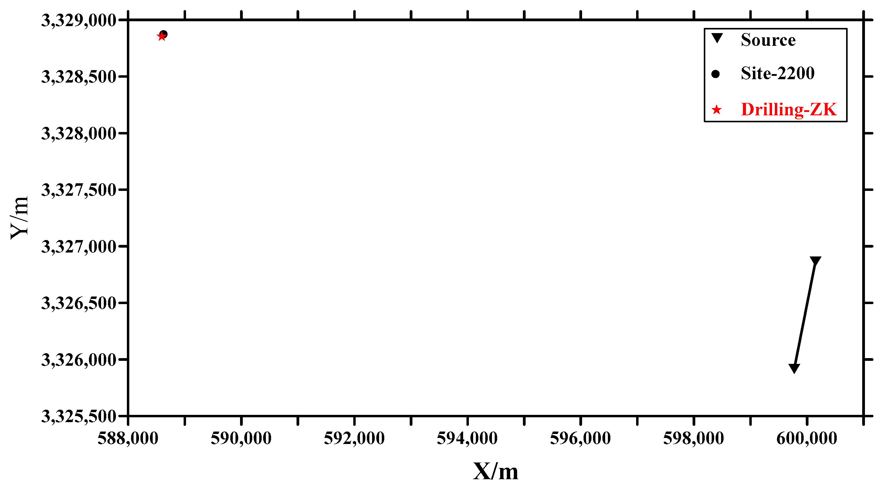
4.3. Practical Application

To further verify the effectiveness of the proposed algorithm, we applied it to the processing of measured CSEM data from the Southeastern Hubei Mineral District. The study area’s stratigraphy primarily consists of Quaternary deposits, the Lower Cretaceous Dasi Formation (K1d), and the Lower–Middle Triassic formations, including the Jialing Jiang Formation (T1-2j) and Daye Formation (T1d). And the Tonglüshan Cu-Fe deposit is a typical skarn-type copper–iron deposit, whose orebody occurrence is controlled by the Tonglüshan anticlinal marble remnant and the Tonglüshan quartz monzonite porphyry. The marble remnant of the Tonglüshan Anticline generally extends in an NNE (north–north-east) trend. Orebodies primarily occur along the intrusive rock–marble contact zone, secondarily within interlayered marble beds near the contact, and rarely within the intrusive rock adjacent to the contact. The reliability of the algorithm presented in this paper was validated using the measured data from survey point 2200 near borehole ZK. The transmitter length was 1021.006 m, the transmission current was 112 amperes, and the offset was 11.6 km. The frequency range spanned from 3/256 Hz to 8192 Hz, comprising a total of 61 frequency points (units: Hz). The field-measured data represent the potential difference between receiving electrodes, from which the horizontal electric field component can be derived by calculating the ratio of potential difference to electrode spacing.

4.3.1. Induced Polarization Logging Results of Borehole ZK

IP (induced polarization) logging was conducted in the borehole across the interval from 30 to 1100.00 m. The dominant lithologies encountered include (Chalcopyrite-mineralized) quartz monzonite diorite porphyry, Chalcopyrite-mineralized dolomitic marble, copper–iron ore bodies, and marble. The layered resistivity and chargeability data obtained from the IP logging are presented in

Table 3. Apparent resistivity and chargeability from IP logging in Borehole ZK.

Depth (m)	Lithology	Resistivity (Ω·m)	Polarizability
20.00–671.92	Quartz Monzodiorite Porphyry	2184.00	5.00%
–686.32	Chalcopyrite-mineralized Quartz Monzodiorite Porphyry	1108.8	12.3%
–727.16	Quartz Monzodiorite Porphyry	1808	5.00%
–762.76	Chalcopyrite-mineralized Dolomitic Marble	524.59	12.15%
–777.96	Copper–Iron Ore Body	40.03	29.15%
–1031.80	Marble	491.82	5.00%
–1040.40	Quartz Monzodiorite Porphyry	118.03	9.28%
–1049.00	Copper–Iron Ore Body	65.35	28.56%
–1104.50	Quartz Monzodiorite Porphyry	573.65	8.19%

.

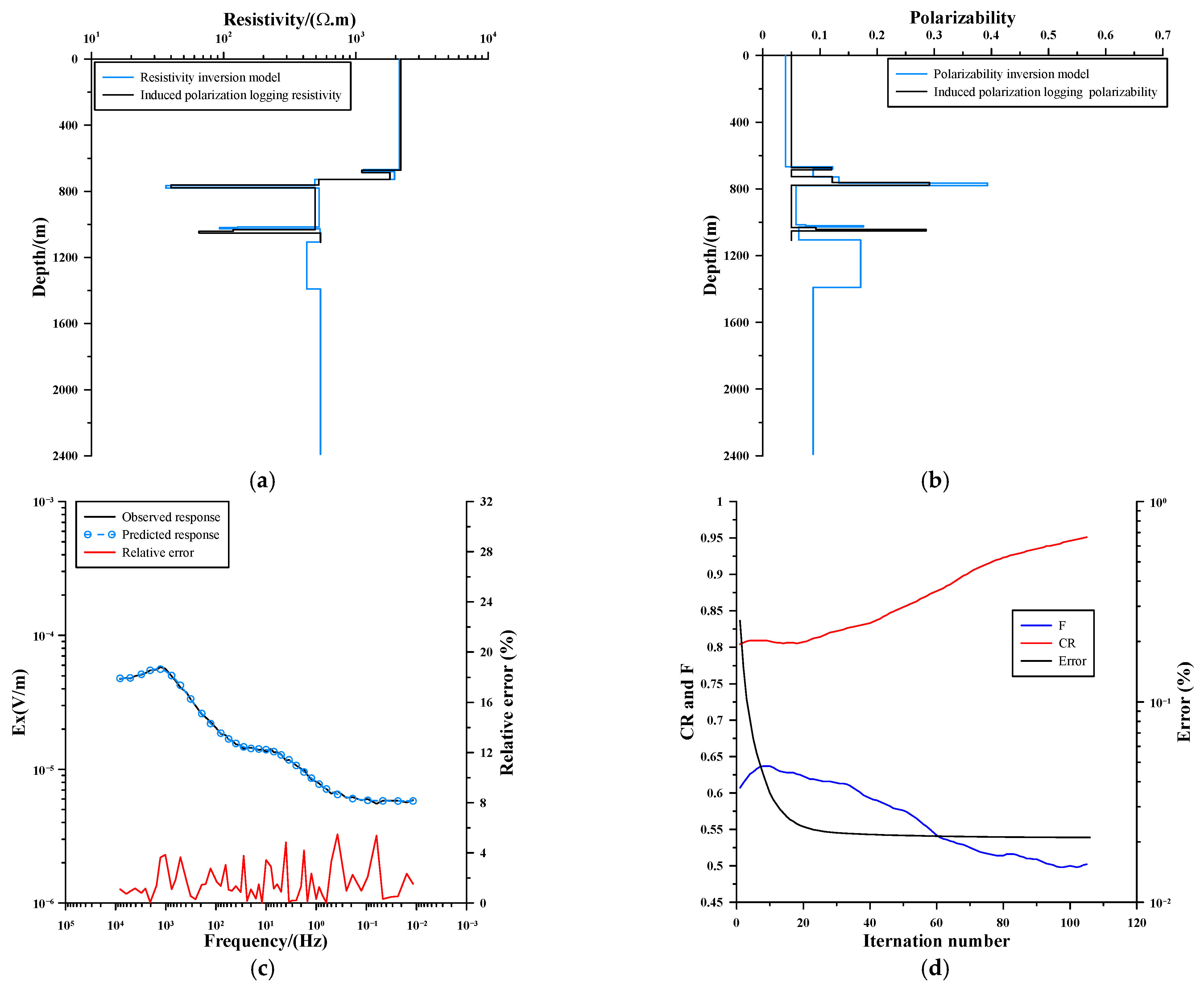
4.3.2. Inversion of Survey Points Adjacent to Borehole ZK

To validate the applicability of the proposed algorithm, inversion was performed using the measured data from Survey Point 2200 near the borehole. In this paper, the initialization parameters are as follows. The number of model parameters is D = 54, and the population size is NP = 220. The regularization parameter is set to $\lambda =0.5$, and the initial values for ${\mu }_{CR}$ and ${\mu }_F$ are 0.8 and 0.6, respectively. Constants c and p are set to 0.1. The inversion results are presented in Figure 8.

Figure 9a,b present comparative analyses of the inversion-derived resistivity and chargeability results at Survey Point 2200 against the borehole induced polarization (IP) logging data. The inversion results of both resistivity and chargeability show strong consistency with the borehole IP logging data and align well with the known ore body parameters, demonstrating the effectiveness of the proposed algorithm. Figure 9c presents the fitting results between the predicted Ex response from the inversion model and the measured Ex response, demonstrating excellent agreement across the entire frequency range. Figure 9d displays the inversion iteration error curve, demonstrating stable convergence as the error consistently decreases with increasing iterations.

5. Conclusions

In this study, we used the adaptive differential evolution algorithm to effectively extract resistivity and polarization information from the CSEM. Our results showed that (1) the proposed algorithm was able to accurately extract resistivity and polarization information from layered geoelectric models and accurately reconstruct them—particularly in terms of extracting polarization information from the middle layer of a typical three-layer model. (2) It was able to accurately reflect the low-resistivity, high-polarization information of the target layer when applied to both theoretical and real-world geoelectric models—even when the data were perturbed by the introduction of 20% random noise, thus demonstrating a strong resistance to interference. (3) For field-measured data, the proposed method demonstrates strong agreement with the known borehole resistivity and chargeability data, confirming the algorithm’s high applicability in accurately extracting resistivity and chargeability parameters from real data.

The adaptive differential evolution method proposed in this study has exhibited high levels of stability and resistance to the effects of signal noise, making it potentially suitable for applications involving the processing of real-world controlled-source frequency-domain electromagnetic data, potentially spanning multiple fields related to navigation, wherein geoelectric factors, potentially caused by underground ore or metallic deposits, should be considered.

However, owing to the complexity of real-world geoelectric structures and the presence of complex noise in real-world scenarios, the application of this method to the inversion of data taken from the field may nevertheless face the following challenges: ① In applications that involve a higher number of target model layers, the inversion process may be time-consuming. Thus, multiple inversion algorithms may need to be developed and deployed in parallel. ② The inversion method developed in this study is fully nonlinear. Although the minimum structure constraint was introduced, the challenge of non-uniqueness persists, owing to the high number of inversion parameters. Future work in this field should consider using seismic and logging data to address constraints related to layer positions, as this may significantly reduce the non-uniqueness of the solution and the computation time for the inversion calculation.

References

1. Bertin, J.; Loeb, J.; Chen, L. Experiments and Theory of Induced Polarization; Geological Press: Beijing, China, 1980. [Google Scholar]
2. Xu, W.D.; Che, Y.J. On IP Effect of Multi-polarization Layers from CSAMT. J. Eng. Geophys. 2012, 9, 511–515. [Google Scholar]
3. Tang, J.T.; Huang, L.; Yu, C.L. The responsibility of apparent resistivity curves on CSAMT for polarized layer. Chin. J. Eng. Geophys. 2008, 5, 648–651. [Google Scholar]
4. Yue, A.P.; Di, Q.Y.; Wang, M.Y.; Shi, K.F. 1D forward simulation of MT induced polarization (IP) effect of reservoir. Oil Geophys. Prospect. 2009, 44, 364–370. [Google Scholar]
5. Yue, A.P.; Di, Q.Y.; Wang, M.Y.; Shi, K.F. 1-D forward modeling of the CSAMT signal incorporating IP effect. Chin. J. Geophys. 2009, 52, 1937–1946. (In Chinese) [Google Scholar] [CrossRef]
6. Yu, C.T. 2D Forward Modeling and Joint Inversion of the CSAMT Signal Incorporation IP Effect. Ph.D. Thesis, Taiyuan University of Technology, Taiyuan, China, 2012. [Google Scholar]
7. Wang, J.L.; Liu, M.W.; Li, D.; Li, J.H.; Lin, P.R.; Wang, M. Finite element numerical simulation on line controlled source based on Cole-Cole model. Comput. Tech. Geophys. Chem. Explor. 2015, 37, 32–39. [Google Scholar]
8. Huang, Y.W. 3D Forward Modeling and Response Analysis of the Controlled Source Electromagnetic Signal with IP Effect. Master’s Thesis, East China University of Technology, Nanchang, China, 2017. [Google Scholar]
9. Cheng, J.Z. Study and Application of Full-Parameter Inversion Method in Time-Frequency Electromagnetic Method. Master’s Thesis, Yangtze University, Wuhan, China, 2018. [Google Scholar]
10. Joost, H.; Grigory, G.; Konstantin, T.; Andreas, K. Conversion of induced polarization data and their uncertainty from time domain to frequency domain using Debye decomposition. Minerals 2023, 13, 955. [Google Scholar] [CrossRef]
11. He, H.Y.; Wang, J.R.; Wen, W.; Tian, R.C.; Lin, J.S.; Huang, W.Q.; Li, Y.B. Deep structure of epithermal deposits in Youxi area: Insights from CSAMT and Dual—Frequnency IP data. Minerals 2024, 14, 27. [Google Scholar] [CrossRef]
12. Dong, L.; Jiang, F.B.; Li, D.Q. IP extraction from magnetotelluric sounding data based on adaptive differential evolution inversion. Oil Geophys. Prospect. 2016, 51, 613–624. [Google Scholar] [CrossRef]
13. Yoshioka, K.; Zhdanov, M.S. Three-dimensional nonlinear regularized inversion of the induced polarization data based on the Cole-Cole model. Phys. Earth Planet. Inter. 2005, 150, 29–43. [Google Scholar] [CrossRef]
14. Liu, L.; Chang, Y.J.; Cao, Z.L. Research on induced polarization effect of CSAMT on polarizable horizontal layer. Chin. J. Eng. Geophys. 2008, 5, 686–690. [Google Scholar]
15. Huang, L. Extract IP Effect from CSAMT. Master’s Thesis, Central South University, Changsha, China, 2009. [Google Scholar]
16. Xu, W.D. Study on Effection and Application of IP from CSAMT. Ph.D. Thesis, Jilin University, Changchun, China, 2011. [Google Scholar]
17. Feng, B.; Wang, J.L.; Zhang, J.F.; Duan, M.J. The preliminary exploration to extract the IP effect which using CSAMT electromagnetic field response method. Prog. Geophys. 2013, 28, 2116–2122. [Google Scholar] [CrossRef]
18. Xu, Y.C. 1D Forward Modeling and Inversion of the CSAMT Signal Incorporation IP Effect. Master’s Thesis, Chengdu University of Technology, Chengdu, China, 2016. [Google Scholar]
19. Storn, R.; Price, K. Differential evolution—A simple and efficient heuristic for global optimization over continuous spaces. J. Glob. Optim. 1997, 11, 341–359. [Google Scholar] [CrossRef]
20. Pan, K.J.; Wang, W.J.; Tan, Y.J.; Cao, J.X. Geophysical linear inversion based on hybrid differential evolution algorithm. Chin. J. Geophys. 2009, 52, 3083–3090. (In Chinese) [Google Scholar] [CrossRef]
21. Xiong, J.; Meng, X.H.; Liu, C.Y.; Peng, M. Magnetotelluric inversion based on differential evolution. Geophys. Geochem. Explor. 2012, 36, 448–451. [Google Scholar]
22. Zeng, Z.W.; Chen, X.; Yang, H.Y.; Zhang, Z.Y.; Guo, Y.H.; Liu, X.; Ye, Y.X. Joint inversion of magnetotelluric and gravity based on improved differential evolution algorithm and wide-range petrophysical constraints. Chin. J. Geophys. 2020, 63, 4565–4577. (In Chinese) [Google Scholar] [CrossRef]
23. Wang, T.Y.; Hou, Z.; He, Y.X.; Yang, J.; Chao, M.N.; Liu, G.H. Magnetotelluric inversion based on the improved differential evolution algorithm. Prog. Geophys. 2022, 37, 1605–1612. [Google Scholar] [CrossRef]
24. Kenneth, S.C.; Robert, H.C. Dispersion and absorption in dielectrics I. Alternating current characteristics. J. Chem. Phys. 1941, 9, 341–351. [Google Scholar] [CrossRef]
25. Pelton, W.H.; Ward, P.G.; Half, P.G.; Sill, W.R.; Nelson, P.H. Mineral discrimination and removal of inductive coupling with multifrequency IP. Geophysics 1978, 43, 588–609. [Google Scholar] [CrossRef]
26. Liu, Y. 2D Finite Element Modeling and Inversion for Marine Controlled-Source Electromagnetic Fields. Ph.D. Thesis, Ocean University of China, Qingdao, China, 2014. [Google Scholar]
27. Zhang, J.Q.; Sanderson, A.C. JADE: Adaptive differential evolution with optional external archive. IEEE Trans. Evol. Comput. 2009, 13, 945–958. [Google Scholar] [CrossRef]
28. Chen, X.B.; Zhao, G.Z.; Tang, J.; Zhan, Y.; Wang, J.J. An adaptive regularized inversion algorithm for magnetolluric data. Chin. J. Geophys. 2005, 48, 937–946. (In Chinese) [Google Scholar] [CrossRef]
29. Brest, J.; Greiner, S.; Boskovic, B.; Mernik, M.; Zumer, V. Self-adapting control parameters in differential evolution: A comparative study on numerical benchmark problems. IEEE Trans. Evol. Comput. 2006, 10, 646–657. [Google Scholar] [CrossRef]
Figure 1. Flowchart of the adaptive differential evolution inversion algorithm.
Minerals 15 00754 g001
Figure 2. Inversion results of the CSEM for the H-type geoelectric model: (a) resistivity, (b) polarizability, (c) time constant, (d) frequency-dependent coefficient, (e) E x data fitting curve and relative error at each frequency, and (f) inversion-related data information curve.
Minerals 15 00754 g002
Figure 3. Inversion results of the CSEM for the K-type geoelectric model: (a) resistivity, (b) polarizability, (c) time constant, (d) frequency-dependent coefficient, (e) E x data fitting curve and relative error at each frequency, and (f) inversion-related data information curve.
Minerals 15 00754 g003
Figure 4. Inversion results of the CSEM for the A-type geoelectric model: (a) resistivity, (b) polarizability, (c) time constant, (d) frequency-dependent coefficient, (e) E x data fitting curve and relative error at each frequency, and (f) inversion-related data information curve.
Minerals 15 00754 g004
Figure 5. Inversion results of the CSEM for the Q-type geoelectric model: (a) resistivity, (b) polarizability, (c) time constant, (d) frequency-dependent coefficient, (e) E x data fitting curve and relative error at each frequency, and (f) inversion-related data information curve.
Minerals 15 00754 g005
Figure 6. Inversion results of the CSEM for the real-world geoelectric model: (a) resistivity, (b) polarizability, (c) time constant, (d) frequency-dependent coefficient, (e) E x data fitting curve and relative error at each frequency, and (f) inversion-related data information curve.
Minerals 15 00754 g006
Figure 7. Inversion results of the CSEM for the real geoelectric model with the introduction of 20% noise: (a) resistivity, (b) polarizability, (c) time constant, (d) frequency-dependent coefficient, (e) E x data fitting curve and relative error at each frequency, and (f) inversion-related data information curve.
Minerals 15 00754 g007aMinerals 15 00754 g007b
Figure 8. Field data acquisition schematic diagram.
Minerals 15 00754 g008
Figure 9. Inversion results of the CSEM for the real data: (a) resistivity inversion result, (b) polarizability inversion result, (c) E x data fitting curve and relative error at each frequency, and (d) inversion-related data information curve.
Minerals 15 00754 g009