Transformer–GCN Fusion Framework for Mineral Prospectivity Mapping: A Geospatial Deep Learning Approach

Abstract

Mineral prospectivity mapping (MPM) is a pivotal technique in geoscientific mineral resource exploration. To address three critical challenges in current deep convolutional neural network applications for geoscientific mineral resource prediction—(1) model bias induced by imbalanced distribution of ore deposit samples, (2) deficiency in global feature extraction due to excessive reliance on local spatial correlations, and (3) diminished discriminative capability caused by feature smoothing in deep networks—this study innovatively proposes a T-GCN model integrating Transformer with graph convolutional neural networks (GCNs). The model achieves breakthrough performance through three key technological innovations: firstly, constructing a global perceptual field via Transformer’s self-attention mechanism to effectively capture long-range geological relationships; secondly, combining GCNs’ advantages in topological feature extraction to realize multi-scale feature fusion; and thirdly, designing a feature enhancement module to mitigate deep network degradation. In practical application to the PangXD ore district, the T-GCN model achieved a prediction accuracy of 97.27%, representing a 3.76 percentage point improvement over the best comparative model, and successfully identified five prospective mineralization zones, demonstrating its superior performance and application value under complex geological conditions.

1. Introduction

With the rapid development of modern technology, the exploration and development of mineral resources, as a critical guarantee for national economic security and strategic development, has garnered increasing attention [1,2,3,4]. Currently, mineral resource exploration faces unprecedented challenges: the shift from shallow deposits to deep-seated ore bodies, covered areas, and concealed deposits has driven a transformation in exploration methods from traditional qualitative analysis to artificial intelligence (AI)-based quantitative prediction [5,6]. This transformation urgently demands research on new technical approaches. In the field of mineral deposit resource estimation, the development of professional geological software has significantly enhanced the scientificity and efficiency of exploration work. The current mainstream industry tools include Surpac, Micromine, 3DMine, Prospector MRAS, GoCAD, and Studio RM [7,8,9]. These software solutions integrate geostatistics, 3D modeling, and data visualization technologies, driving the research on mineral resource prediction toward a direction of high precision and intelligence, and providing important technical support for deep resource exploration and development.

In the geosciences, AI technologies are propelling a leap in mineral prospectivity prediction methods from traditional statistical models to intelligent algorithms [10,11]. Compared with conventional statistical methods, machine learning and deep learning algorithms have demonstrated remarkable advantages in revealing complex nonlinear relationships [12,13,14,15,16,17]. These intelligent algorithms can effectively integrate multi-source heterogeneous data, such as geological, geophysical, geochemical, and remote sensing data, to construct high-precision prediction models [18,19,20]. For example, Cao et al. [21] proposed an attention-driven graph convolutional neural network for mineral prospectivity mapping, achieving an ACC (accuracy) of 83.55% and an AUC (area under the curve) of 91.67%, and successfully predicting mineral prospectivity target areas. Cao et al. [22] optimized a random forest model to significantly enhance the identification of geochemical anomaly information related to iron deposits while overcoming some limitations of traditional random forest models. Lachaud et al. [23] established gold prospecting models using two data-driven methods—random forest and support vector machine (SVM)—with both models achieving accuracies exceeding 80%. Ghezelbash et al. [24] applied K-means and SVM for geoscience data-driven classification, successfully mapping copper mineral prospectivity in the Varzaghan region, Iran. Shaw et al. [25] used classification methods such as random forest (RF), K-nearest neighbors (KNN), and SVM to model ore prospectivity areas, demonstrating that RF and KNN models could achieve prediction rates of up to 90%. Xiao et al. [26] proposed a hybrid GEP-LR model that combines LR with gene expression programming (GEP), and conducted a comprehensive data modeling and prospectivity mapping case study on porphyry Cu-Mo polymetallic deposits in the eastern Tianshan Mountains. Li et al. [27] developed a convolutional neural network (CNN)-based method for multi-element geochemical map recognition, which effectively mitigated the small-sample problem through transfer learning and significantly improved model accuracy. These achievements provide critical references for intelligent mineral prediction.

Despite significant progress in current mineral prospectivity prediction research, intelligent prediction models still face three critical challenges: (1) data scarcity: the limited number of known deposits in study areas leads to severe training data imbalance, significantly reducing the generalization capability of deep learning models and impairing classification performance; (2) architectural limitations: existing models overly rely on local spatial correlations, hindering their ability to capture deep-seated geological relationships; and (3) feature smoothing: multi-layer graph convolutional operations induce feature homogenization, diminishing the expressiveness of critical geological features.

To address these challenges, this study innovatively proposes T-GCN, a novel network model integrating Transformer and graph convolutional networks (GCNs) for MPM. The model achieves breakthrough performance through three key innovations: First, a Generative Adversarial Network (GAN) is employed to augment the sample dataset, effectively alleviating the problem of imbalanced data distribution; second, a geochemical element correlation graph is constructed based on an adaptive threshold Pearson correlation coefficient to accurately characterize the interaction relationships between elements; and finally, the global attention mechanism of Transformer is synergistically combined with the local feature extraction capability of GCNs to capture complex spatial patterns and nonlinear relationships. This not only significantly mitigates the feature smoothing issue but also excels in both global spatial feature perception and local feature extraction. Through comparative analysis with multiple classical models, T-GCN demonstrates superior robustness and reliability in terms of prediction accuracy (ACC), anomaly probability maps, and other metrics.

2. Geological Background and Dataset

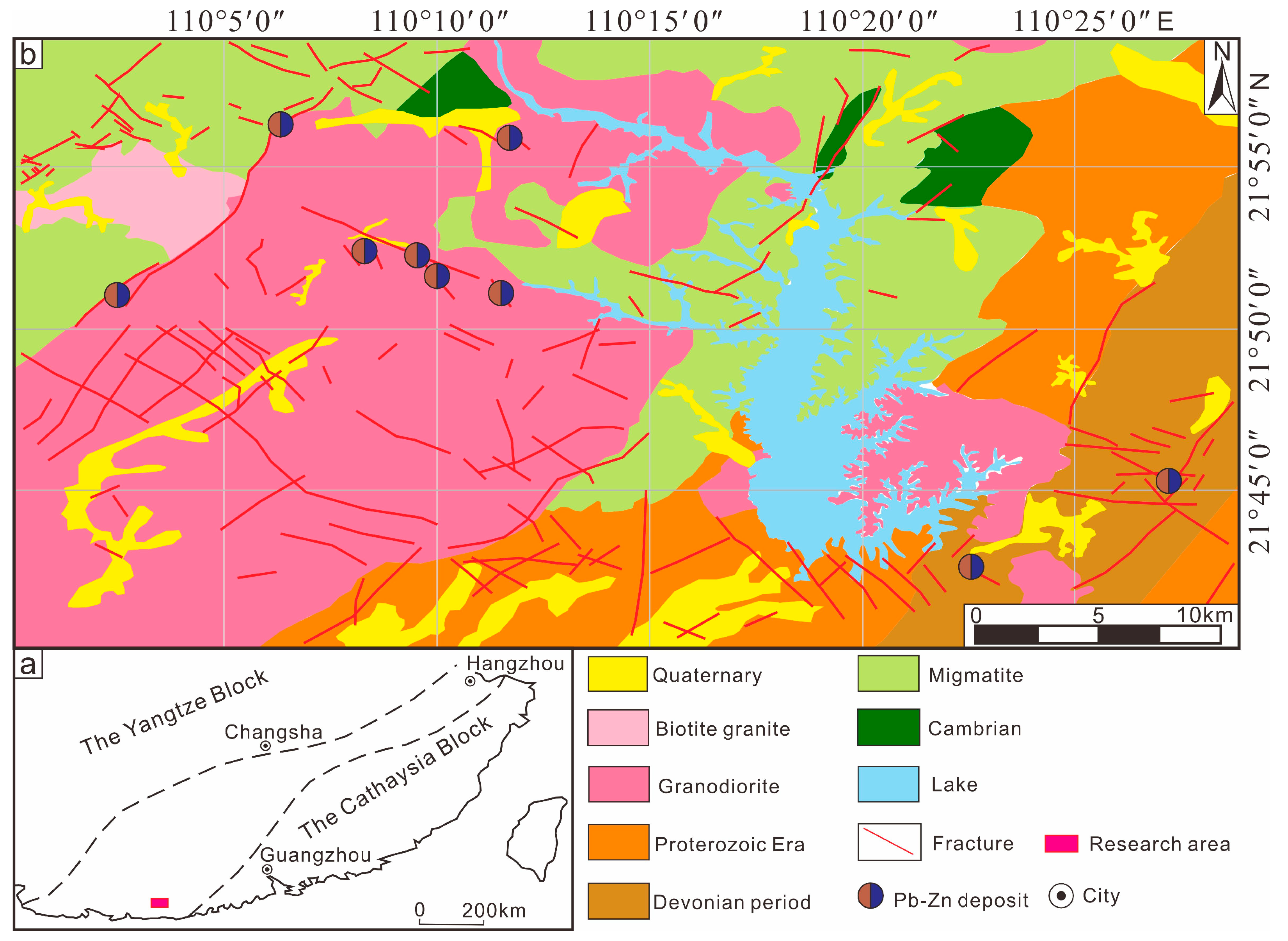
2.1. Geological Background

The PangXD area is located in the southern segment of the Qin-Hang metallogenic belt in China (Figure 1), which represents a significant mineralized zone formed along the ancient subduction boundary between the Yangtze and Cathaysia Block [28,29,30,31]. The region is characterized by significant features, such as large-scale ore deposits, dense distribution of mineral deposits, and complete types of ore deposits, holding important potential for lead–zinc, copper–polymetallic, and gold and silver deposits. The ore bodies exposed in the study area are dominated by lead–zinc deposits, with local interlayers of pyrite. The ore bodies and mineralization zones mostly occur in stratoid or lenticular shapes, extending in an overall NE–SW strike. The mineralization alteration types are abundant, mainly developed with silicification, pyritization, calcitization, dolomitization, chloritization, and galenization. The genetic type of the deposit belongs to the sedimentary hydrothermal reformation-type lead–zinc deposit.

The PangXD area exhibits complex geological structures with frequent and intense magmatic activities, where diverse geological phenomena are well-developed. Intrusive rocks are widely distributed, covering approximately 60% of the total area, predominantly exposed in the central–northern and western sectors. These intrusions are primarily products of Caledonian and Yanshanian magmatic events, occurring mainly as batholiths and stocks, with sporadic granite porphyry dikes. Each phase of magmatic intrusion was controlled by specific tectonic systems. More significantly, the multi-stage magmatic activities were accompanied by significant enrichment of base metals (Pb, Zn, Cu) and precious metals (Au, Ag), forming several economically valuable deposits.

The stratigraphic sequence in the study area is relatively simple but has undergone intense tectonic deformation. The region experienced multiple tectonic episodes, developing various structural features, including faults and folds, with fault structures being the most prominent. The fracture zones serve as the primary ore-controlling structures, whose spatial distribution strictly governs deposit localization. Specifically, the deposits are concentrated within NE- and NW-trending fracture zones and their adjacent areas, particularly at the intersections of these fault systems. This systematic mineralization distribution pattern provides crucial structural constraints for regional prospecting predictions.

2.2. Dataset

The geochemical data for the PangXD area were obtained from the China Geological Survey program [32,33]. This study selected stream sediments as the sampling medium, with an average sampling density of 4.25 samples per square kilometer. The sampling covered a total area of 1694 square kilometers, yielding 7236 samples. Each sample was analyzed for 16 elements: Au, B, Sn, Cu, Ag, Ba, Mn, Pb, Zn, As, Sb, Bi, Hg, Mo, W, and F.

Table 1. Partial geochemical element data set (the unit of Au and Ag are ng/g, other elements unit are μg/g).

X	Y	Ag	Au	B	Sn	Cu	Ba	Mn	Pb	Zn	As	Sb	Hg	Mo	W	Bi	F
421.63	2416.85	0.078	0.54	4	2.56	7	88	209	12	23	0.9	0.29	0.04	0.82	1.16	0.42	204
420.93	2416.80	0.06	0.81	3	3.74	5	885	305	33	22	0.58	0.36	0.04	0.82	1.11	1.41	222
420.95	2416.35	0.086	0.94	4	2.41	5	797	267	53	35	1.15	0.34	0.09	0.51	1.16	0.42	212
421.21	2415.85	0.043	0.81	3	1.52	5	1111	423	42	14	0.51	0.35	0.07	0.59	0.38	0.23	222
420.30	2416.35	0.046	0.37	2	1.65	6	941	498	38	17	0.53	0.31	0.02	0.57	0.33	0.61	222
419.86	2416.15	0.033	1.09	4	1.53	8	427	338	37	29	0.74	0.28	0.07	1.68	0.73	0.47	204

shows part of the geochemical element data, and X and Y correspond to the sampling point coordinates. Figure 2 illustrates the spatial distribution of Pb–Zn elements in the study area.

2.3. Data Characteristic Analysis

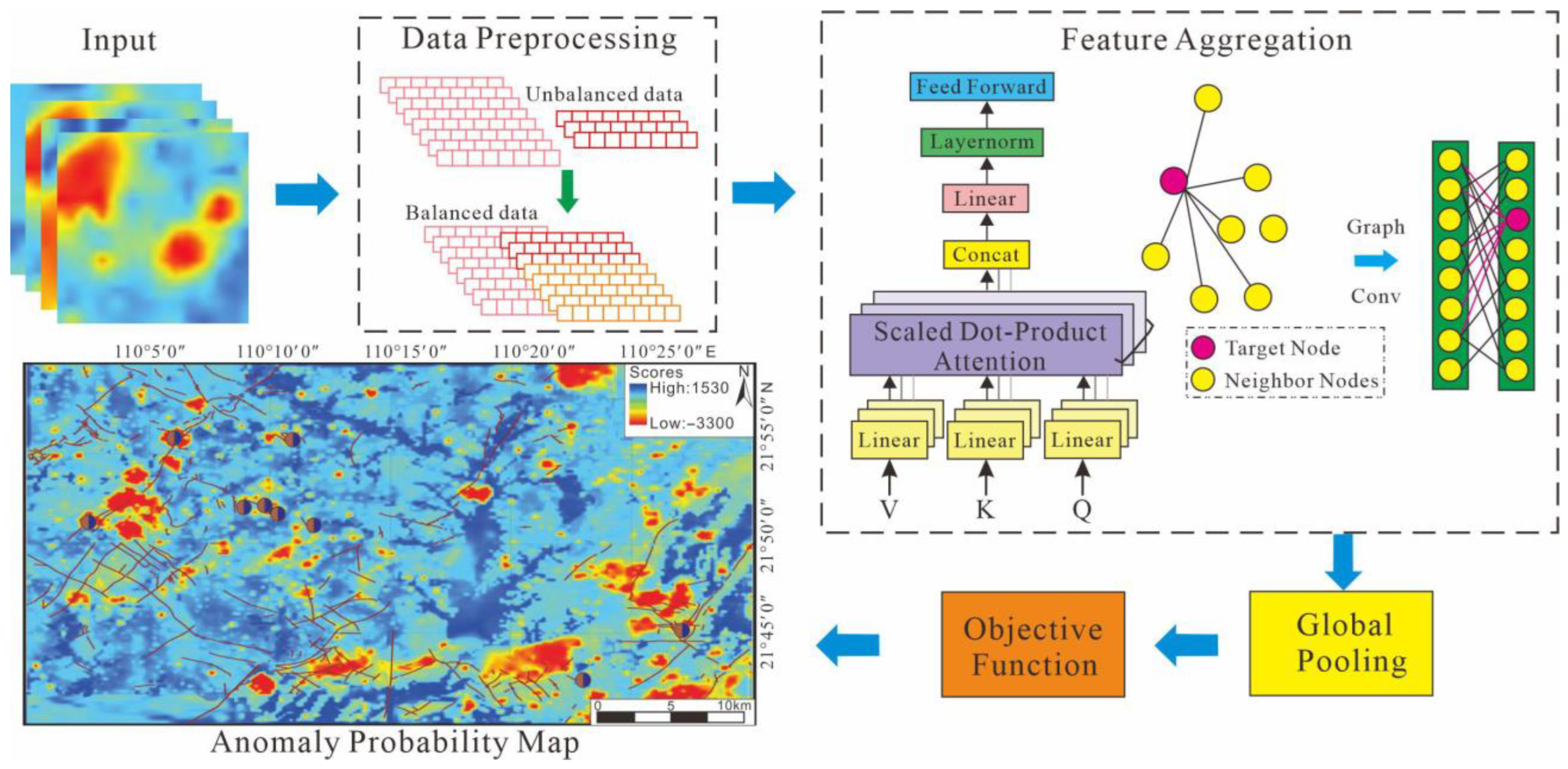
This study systematically analyzed the statistical characteristics of 16 key geochemical elements (Pb, Zn, Au, Ag, Cu, etc.) in the PangXD study area (

Table 2. Statistical information on the data for the 16 elements.

Element (mg/kg−1)	Maximum Value	Minimum Value	Mean Value	Standard Deviation	Coefficient of Variation
Au	1.145	0.2 × 10−3	2.06 × 10−3	0.019	9.5
B	950	1	38.92	50.82	1.39
Sn	280	0.85	4.99	6.92	1.4
Cu	440	1	12.01	16.82	1.31
Ag	40.7	0.04	0.63	0.59	0.94
Ba	1872	6	200.72	188.7	7
Mn	3183	49	345.33	199.68	0.578
Pb	5504	1	34.57	74.3	2.57
Zn	2955	3	36.11	50	5.35
As	1520	0.1	6.11	22.85	2.72
Sb	2610	0.14	0.89	30.69	0.62
Bi	250	0.01	0.98	3.97	2.15
Hg	14.5	0.03	0.07	0.19	1.39
Mo	407.59	0.12	1.69	9.01	3.74
W	511	0.14	3.18	8.64	34.43
F	3930	33	300.95	185.12	4.06

). The results reveal that (1) the elemental concentrations exhibit significant magnitude differences, with the maximum-to-mean ratios exceeding 200-fold for ore-forming elements, including Au, Ag, As, Sb, Bi, and Mo, indicating potential local anomalies; (2) the coefficient of variation (CV) analysis demonstrates that most elements have CV values >1 (particularly critical ore-forming elements like Au and Ag, with CVs of 9.2 and 7.0, respectively), reflecting strong spatial variability and significant local enrichment of these elements, which provides important prospecting indicators [34]; and (3) integrated with regional geological background analysis, this high variability characteristic shows close correlation with multi-stage hydrothermal activities in the study area, further evidencing favorable metallogenic conditions and considerable resource exploration potential.

3. Methods

The proposed methodology for mineral prospectivity mapping is based on the Transformer–GCN fusion framework (Figure 3). The proposed framework innovatively integrates compositional data analysis techniques with state-of-the-art graph convolutional neural networks, enabling effective capture of complex nonlinear spatial correlations among geological features.

3.1. Data Preprocessing

3.1.1. Data Transformation

Geochemical data are typically regarded as compositional data, where the sum of individual element contents is a fixed value. However, such data may generate a closure effect, leading to significant correlations between interdependent elements. Therefore, when analyzing geochemical data, some statistical techniques may trigger data correlation issues due to ignoring data constraints.

To address the above problems, this study employs data preprocessing techniques to transform original compositional data into logarithmic scales. This operation not only significantly reduces the interference of outliers on analysis results but also makes the data distribution characteristics more approximate to a normal distribution, laying a good foundation for subsequent analysis. Currently, there are mainly two preprocessing methods for such data:

The first is the Additive Log Ratio Transformation (ALR). Based on logarithmic functions, this method is often used to process data with proportional relationships. By converting the proportional relationships in the original data into additive relationships, it significantly simplifies the statistical analysis and model construction processes. For a vector of relative abundance data $x=\left[x_1,x_2,\dots ,x_k\right]$ containing k components, a specific component is selected as the reference. The ALR transformation of each remaining component $x_i(i=1,2,\dots ,k-1)$ is defined as the natural logarithm of the ratio of the component to the reference component. Its mathematical expression is expressed as Equation (1):

$$\mathrm{A}\mathrm{L}\mathrm{R}(x_i)=\mathrm{l}\mathrm{o}\mathrm{g}({\displaystyle \frac{x_i}{x_k}})\mathrm{f}\mathrm{o}\mathrm{r}i=1,2,\dots ,k-1$$

(1)

where $x_i$ represents the value of the i-th component in the vector, $x_k$ denotes the value of the reference component chosen as the denominator, and the last component is typically selected as the reference. Existing studies have shown that ALR transformation can effectively improve data structure and facilitate subsequent quantitative analysis [35].

The second is the Centered Log Ratio Transformation (CLR). This method can convert information in multivariate datasets into log-ratio forms, which not only effectively eliminates the scale effect in the data but also standardizes the data into log-ratio forms with a unified reference based on the data center. The CLR transformation formula is shown as Equation (2):

$$\mathrm{C}\mathrm{L}\mathrm{R}\left(x_i\right)=\mathrm{l}\mathrm{n}({\displaystyle \frac{x_i}{g}})$$

(2)

where $x_i$ is a component in the compositional data, and g is the geometric mean of all components. This transformation method not only helps reveal the potential relationships between data but also improves the accuracy and reliability of data analysis results [36].

Through preprocessing of the original data, this study effectively improved the data distribution characteristics. As shown in the violin plots (Figure 4) and density curves (Figure 5), the original data exhibited significant spatial scale differences, discrete distributions, and high-value anomalies in most elements. After logarithmic transformation and CLR transformation, the scale differences in element spatial distribution were significantly reduced, box plots showed more uniform distributions, and density curves approached unimodal or multimodal normal distributions. Comparing the data characteristics after the two transformations, the CLR-transformed data (Figure 4c) showed more concentrated and balanced spatial scales and internal dispersion, more symmetrical high–low extreme value distributions, and density distributions closer to the standard normal distribution (Figure 5) compared to the logarithmically transformed data (Figure 4b). This indicates that data transformation significantly alleviated the internal heterogeneity of the dataset, eliminated skewed distributions, and improved data concentration, laying a good foundation for multivariate statistical analysis. Compared with logarithmic transformation, CLR transformation was more effective in reducing internal data heterogeneity and shaping normal distribution characteristics.

The reasons for selecting the 25%–75% interquartile range (IQR) in data transformation can be explained from two aspects: (1) statistical perspective: this interval covers 50% of the core samples, effectively filtering outliers such as high-grade mineralization points and measurement errors. This enables box plots/violin plots to more authentically reflect the central tendency and dispersion degree of the data, and (2) compositional data processing: when data represent multi-element content ratios, traditional transformations are affected by the “closure effect”. The CLR transformation eliminates this effect through logarithmic ratios. At this point, IQR variations reflect the distribution law of relative element ratios rather than the dispersion of absolute contents, facilitating effectiveness comparisons among different transformation methods.

3.1.2. Generative Adversarial Network (GAN)

In geographical space, ore deposits exhibit significant sparsity. The number of mineralized indicator samples (Class A) in a specific study area is typically much lower than that of non-mineralized samples (Class B), resulting in pronounced class imbalance in datasets used for numerical modeling of mineral exploration prospectivity maps. To address this issue, this study employs GAN to effectively augment samples from underrepresented classes.

A GAN is a canonical deep learning framework composed of two neural networks: a Generator and a Discriminator [37]. As shown in Figure 6, the Generator synthesizes data samples that approximate the true distribution from random noise, while the Discriminator, acting as a binary classifier, distinguishes whether an input sample is genuine (from the real dataset) or fake (generated by the Generator). The two networks engage in adversarial training: As the Generator improves its ability to produce realistic samples, the Discriminator concurrently enhances its discriminative power. This competitive process culminates in the Generator generating high-fidelity synthetic samples, effectively mitigating class imbalance in the original dataset.

During the GAN training phase, the loss functions for the Generator and Discriminator are denoted as G_loss and D_loss, respectively. Owing to the fact that known ore deposits in the study area constitute only a negligible proportion of the overall training data, the training data for mineral prospectivity prediction models exhibit significant imbalance. When conducting numerical modeling for mineralization prediction on imbalanced datasets, the numerical disparity between minority-class mineralized indicator samples (Class A) and majority-class non-mineralized samples (Class B) can cause the critical information carried by Class A samples to be obscured by Class B samples. This phenomenon may lead algorithms to overfit majority-class sample points while undervaluing the importance of Class A samples. To tackle these challenges, this study proposes a solution of using GAN for data augmentation of Class A samples, aiming to balance data distribution and enhance the model’s capability to represent rare samples.

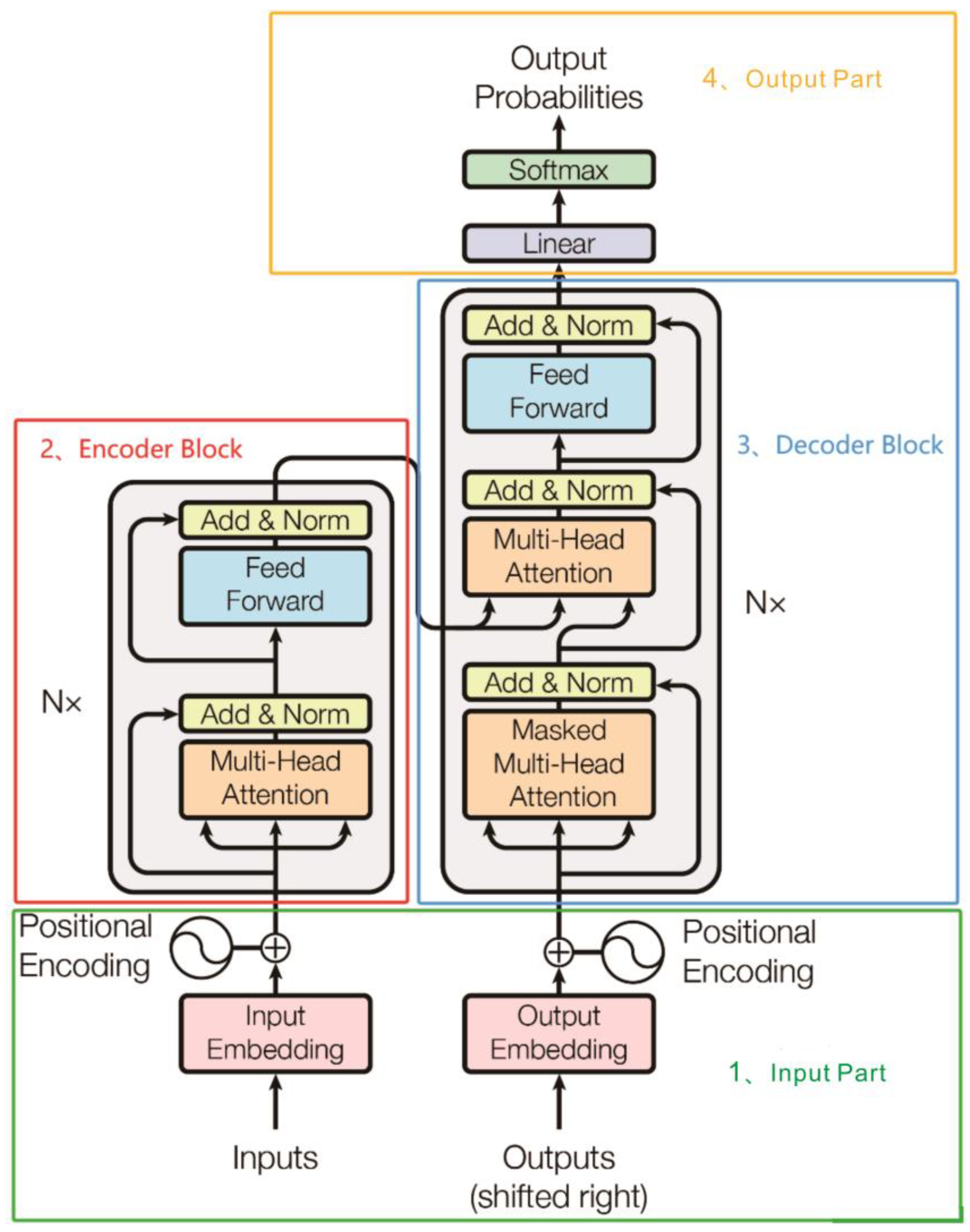
3.2. Transformer Module

The Transformer model is a deep learning architecture based on the self-attention mechanism [38], whose core advantage lies in dynamically assigning attention weights to different parts of the input sequence through the self-attention mechanism, thereby efficiently capturing semantic correlations. In the geological image data, the degree of the labeled mineral point image and different geological prospecting factors can correspond to the weight coefficient. This study will focus on the application of its attention mechanism in mineralization information extraction. The overall architecture of Transformer can be divided into four parts (Figure 7), including the input part, encoder block, decoder block, and output part.

3.2.1. Input Part

The input module consists of multiple functional components:

(1)

Source Text Embedding Layer: Converts the numerical representations of words in the source text into vector representations, capturing semantic associations and contextual relationships between words.

(2)

Positional Encoding Layer: Generates a unique positional vector for each position in the input sequence, enabling the model to perceive positional relationship information within the sequence.

(3)

Target Text Embedding Layer (Decoder-only): Performs the same vectorization operation as the source text on the target text, converting numerical word representations into vector representations containing semantic information to provide the basic input for the decoding process.

3.2.2. Encoder Part

The encoder is composed of N stacked encoder layers. Each encoder layer contains three core modules: multi-head attention and self-attention, feed-forward neural network (FFN), and residual connection and layer normalization.

(1)

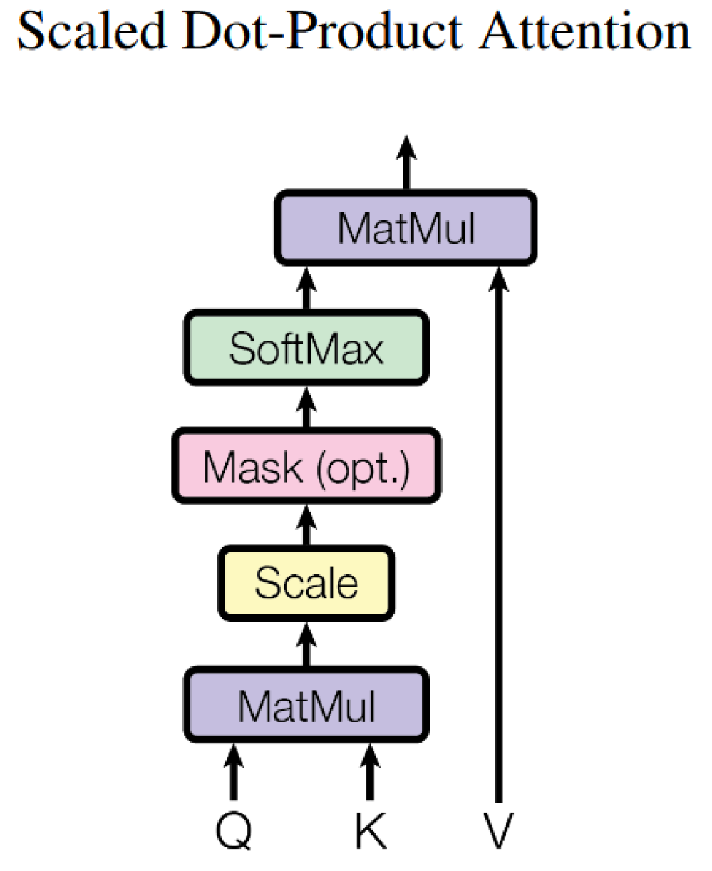
Self-Attention Mechanism: The core of the Transformer architecture enables the model to dynamically focus on the semantic associations of other tokens when processing a specific token. This enhances the ability to capture long-range dependencies and models global semantic relationships. Its structure is shown in Figure 8.

The self-attention calculation involves three key matrices:

The query matrix (Q) represents the information requirements of the current token and is used to match the key matrix.

The key matrix (K) stores the identification information of each token in the input sequence for retrieval by Q.

The value matrix (V) contains the actual semantic information corresponding to K, with relevant V values participating in output calculations when Q matches a K.

Each token undergoes vectorization through trainable weight matrices WQ, WK, and WV, with specific calculations shown in Formulas (3)–(5):

Q = XW_Q

(3)

K = XW_K

(4)

V = XW_V

(5)

Here, X is the input token embedding with dimensions (L, d_model), where L is the sequence length and d_model is the model dimension. W_Q, W_K, and W_V are trainable parameter matrices with dimensions (d_model, d_k).

Based on these matrices, attention weights are calculated using scaled dot-product attention, as shown in Formula (6):

$$\mathit{Attention}(Q,K,V)=\mathit{softmax}({\displaystyle \frac{{QK}^T}{\sqrt{d_k}})V}$$

(6)

Here, QK^T computes the similarity between tokens, and scaling by $\sqrt{{\mathrm{d}}_{\mathrm{k}}}$ avoids gradient explosion. The attention weight matrix is obtained via softmax normalization and then multiplied by the value matrix V to generate the weighted output. The final output matrix is shown in Formula (7):

Z = Attention (Q, K, V)

(7)

The output matrix has dimensions (L, d_model), with each row representing the context-aware representation of a token after self-attention calculation.

(2)

The multi-head attention mechanism is an extension of the self-attention mechanism. By parallelly setting multiple attention heads, the model can learn differentiated attention weights from different semantic subspaces, thereby capturing multi-dimensional semantic associations and feature patterns. Its structure is shown in Figure 9. The specific implementation process is as follows:

Each attention head independently performs self-attention calculations, as shown in Formula (8):

$$Z_h=\mathit{Attention}(Q_h,K_h,V_h)$$

(8)

where h represents the h-th attention head, and Qh, Kh, and Vh are the query, key, and value matrices corresponding to that head. The output results of all heads are then concatenated by dimension, as shown in Formula (9), followed by a unified mapping of the feature space through a linear transformation matrix, as shown in Formula (10):

Z = Concat (Z₁, Z₂, …, Z_h)

(9)

Multi-Head (Q, K, V) = Linear (Concat (Z₁, Z₂, …, Z_h))

(10)

(3)

The FFN consists of two fully connected layers (linear) and a non-linear activation function (ReLU). Its function is to perform non-linear transformations on the features output by the attention mechanism to enhance the model’s ability to express complex semantic patterns. The specific calculation formula is as shown in Formula (11):

$$\mathrm{FFN}\left(\mathrm{x}\right)=\max (0,\mathrm{x}{W}_1+b_1)W_2+b_2$$

(11)

Among them, x is the hidden representation of the input token, with the shape of (B, L, d_model), where B is the batch size, L is the sequence length, and d_model is the model dimension. ${\mathrm{W}}_1$ and ${\mathrm{W}}_2$ are trainable weight matrices, and ${\mathrm{b}}_1$ and ${\mathrm{b}}_2$ are bias terms. By introducing non-linear features, the ReLU activation function enables the model to learn more complex feature interaction relationships.

(4)

Residual connection and layer normalization are applied after the multi-head attention module and the feed-forward neural network module, respectively. Their core roles are to mitigate the gradient vanishing problem in deep networks, accelerate the training process, and prevent excessive modification of feature representations by preserving original input information. The specific calculations are shown in Formulas (12) and (13):

Output = LayerNorm (Input + SubLayer (Input))

(12)

$$\mathit{LayerNorm}(\mathit{x})={\displaystyle \frac{\mathit{x}-\mu }{\sigma +ϵ}}·\gamma +\beta$$

(13)

where x is the input vector with the shape of (B, L, d_model), μ and σ calculate the mean and standard deviation of each sample across the embedding dimension d_model, γ and β are learnable parameters used to scale and shift the normalized values, and ϵ is a small constant to prevent division-by-zero errors.

3.2.3. Decoder Part

The Transformer decoder’s function is sequence generation. It receives the contextual semantic representations output by the encoder and predicts the next token by combining the already generated token sequence. The key difference between the decoder and the encoder lies in the masked multi-head self-attention mechanism. This mechanism ensures that during the decoding process, each token can only attend to the sequence content up to and including the current position by masking future position information, preventing future information leakage and thus adhering to the causal constraints of sequence generation. The masked attention calculation is shown in Formula (14):

$$\mathit{Masked}\mathit{Attention}(Q,K,V)=\mathit{Softmax}({\displaystyle \frac{{QK}^T}{\sqrt{d_k}}}+\mathit{Mask})V$$

(14)

It should be emphasized that to optimize the decoding performance of Transformer, Formula (14) can be modified by adding or multiplying an additional matrix V in specific scenarios. The following constraints need to be noted: (1) the feasibility of adding matrix V, which is only effective when V is used as a residual connection or cross-layer feature fusion, and must be strictly consistent with the original feature dimensions, and (2) application scenarios of multiplying matrix V, which are commonly seen in linear transformation or feature weighting scenarios, but dimension matching should be ensured and computational complexity should be evaluated.

3.2.4. Output Part

The output part consists of a linear layer and a softmax layer:

The linear layer maps the feature vectors (B, L, d_model) output by the decoder to the output dimension of the target task, achieving the transformation from the feature space to the prediction space.

The softmax layer converts the output of the linear layer into a probability distribution, enabling the model to output the prediction probability of each possible token and thus supporting the final decision-making for sequence generation or classification tasks.

This structure ensures that the model’s output conforms to the mathematical properties of the probability space, facilitating subsequent loss calculation and result interpretation.

3.3. GCN Module

Although the Transformer can effectively encode node features and capture a global receptive field through global pooling operations to extract feature representations of the entire graph, it has limitations such as insufficient representation of key nodes and inadequate capture of graph structure information during modeling. To address these issues, this study introduces the GCN model technique to achieve refined node feature representation and in-depth reasoning of graph structure semantics through its local neighborhood aggregation mechanism [39]. The process is illustrated in Figure 10. The red nodes are target nodes, and the blue nodes are neighbor nodes.

The typical input for GCNs comprises an adjacency matrix representing the graph’s topological structure and a node feature a matrix encoding each node’s attribute information. For a graph G = (V, E), where V denotes the node set and E the edge set, each node $v_i$ possesses its own distinct characteristics $x_i$. The node feature matrix can be $X_{N\ast D}$ and the adjacency matrix can be $X_{N\ast N}$, where N denotes the number of nodes and D denotes the number of features for each node.

The GCN module adopts a two-layer GCN architecture, with the output of the Transformer module denoted as ${\mathrm{X}}_{h\mathrm{i}\mathrm{d}\mathrm{d}\mathrm{e}\mathrm{n}}$ serving as the input for the GCNs. The node feature matrix is utilized as the input for the GCNs, while the original graph’s adjacency matrix is employed as the adjacency matrix for the GCN input. Following the graph convolution operation, each node aggregates information from its neighboring nodes to capture the relationships between the node and its surrounding nodes, thereby acquiring a more comprehensive vectorized representation as its own feature representation. All nodes within the GCNs utilize the same weight matrix for information aggregation, enabling the model to exhibit translation invariance for improved handling of graph data. The corresponding mathematical formulation is shown in Formula (15).

$$H^{(l+1)}=\sigma ({\widehat{D}}^{-{\displaystyle \frac{1}{2}}}\widehat{A}{\widehat{D}}^{-{\displaystyle \frac{1}{2}}}{H}^{(l)}{W}^{(l)})$$

(15)

In this equation, the variable $H^{\left(l\right)}$ represents the node representation of the l-th layer, $\widehat{A}=A+I$, $I$ denotes the unit matrix, $\widehat{D}$ stands for the degree matrix of $\widehat{A}$, $W^{\left(l\right)}$ is the weight matrix, $\mathsf{\sigma }(·)$ signifies the activation function, and $H^{\left(0\right)}$ is equivalent to $X_{hidden}$.

The final perceptron layer in the GCNs is tasked with transforming the final node representations into graph-level outputs for classification. This process entails aggregating the node-level representations into graph-level representations through global pooling operations. Subsequently, the graph-level representation is inputted into one or more fully connected layers, typically comprising weight matrices and activation functions. The core function of this layer is to map the graph-level representation to the final classification result.

3.4. Global Pooling

The model employs a global pooling architecture, which is well-suited for processing graph data with diverse structures. At each layer, the feature representation of all nodes is aggregated using the commonly adopted summation-based global pooling method, yielding the feature representation of the entire graph in Formula (16). The final classification result is generated through the softmax activation function.

$$Z_g=READOUT[H_i^1,H_i^1,\dots ,H_i^j],\forall i\in g$$

(16)

where j denotes the number of layers, any node i belongs to the graph g, $G=\{G_1,G_2,\dots ,G_g\}$, and all graphs g belong to the dataset G.

3.5. Objective Function

The cross-entropy loss function is adopted as the objective function for optimization. The expression for the predicted probability and cross-entropy loss function are as follows:

$$\widehat{Y}=softmax(W·Z_g+b)$$

(17)

$$L_{class}=-{\sum }_{gϵG}{\sum }_{c=1}^C{Y}_{gc}ln{\widehat{Y}}_{gc}$$

(18)

where W and b denote the weight matrix and bias vector, respectively; the whole graph represents the $Z_g$; C denotes the number of labeling types of the graph; $Y_{gc}$ denotes the actual label type of graph g; and ${\widehat{Y}}_{gc}$ denotes the predicted label type of graph g. The model optimizes parameters by minimizing the cross-entropy loss function to derive the classification results for graphs.

4. Results and Discussion

4.1. Experimental Setup

This experiment was conducted on a high-performance computing platform, which operates on a 64-bit Windows 10 system, equipped with 32 GB of RAM, an AMD Ryzen 9 4900 H processor, and a Tesla V100 32 GB GPU to accelerate deep learning model training. The experiment was implemented using Python 3.6 programming language and based on the PyTorch 1.7 Geometric deep learning framework.

For the configuration of the Transformer module:

Both the multi-head attention blocks and feed-forward neural network blocks are set to a two-layer architecture, with layer normalization applied before the feature matrix input module. The hidden layer dimensions of the Transformer are set to 64, 128, 256, and 512, respectively. The dropout rate is set to 0.5, and the Adam algorithm is used as the parameter optimizer.

In the hyperparameter tuning phase, this study systematically explored parameters on the training set. Particular emphasis was placed on investigating the impact of the number of convolutional layers (layers) on model performance, with values spanning {2, 4, 8, 16, 32}. Here, a two-layer convolution corresponds to a shallow GCN architecture. To achieve efficient optimization of the model parameters, the Adam optimizer was selected, with an initial learning rate of 0.0005 to precisely control the parameter update step size. To effectively mitigate overfitting, an L2 regularization strategy was introduced, setting the weight decay parameter to 0.0001 to constrain model complexity. Additionally, early stopping was employed as an auxiliary regularization technique: the maximum number of training epochs was set to 200, and a monitoring mechanism was established such that training would terminate early if the validation set loss failed to decrease for 50 consecutive epochs.

In the process of optimizing the residual connection mechanism, fine-tuning was performed on the residual input proportion parameter α and the ratio parameter β between the initial residual and high-order neighborhood residuals, both constrained within the range of 0 to 1. Through parameter micro-adjustments, the impact of different residual strategies on the model’s generalization ability and stability was investigated. Simultaneously, the γ parameter was adjusted to control the sparsity of edges in the graph structure, thereby optimizing graph connectivity and information propagation efficiency.

When constructing the geoscientific image dataset for the study area, a sliding window was defined and an appropriate step size was selected to perform traversal sampling on the images so as to obtain the element content information of each sampling point. After optimization through multiple sets of comparative experiments, it was finally determined to adopt a 128 × 128 (specification) sliding window to carry out spatial sampling operations on the comprehensive geoscientific information map, thereby generating a standardized geoscientific image dataset that is adapted to the needs of model training.

To comprehensively evaluate the model’s effectiveness, this study employed a ten-fold cross-validation approach: the complete dataset was evenly partitioned into 10 subsets to ensure consistent sample sizes across subsets. In each validation iteration, one subset was randomly selected as the validation set, while the remaining nine subsets formed the training set. This process was repeated 10 times to ensure that each subset served as the validation set exactly once. This method generated diverse validation set combinations, enabling a comprehensive assessment of model performance. Finally, the arithmetic mean of the results from the ten validation rounds was computed to obtain stable performance metrics, effectively reducing the randomness inherent in the evaluation results.

4.2. Comparison of Data Augmentation Methods

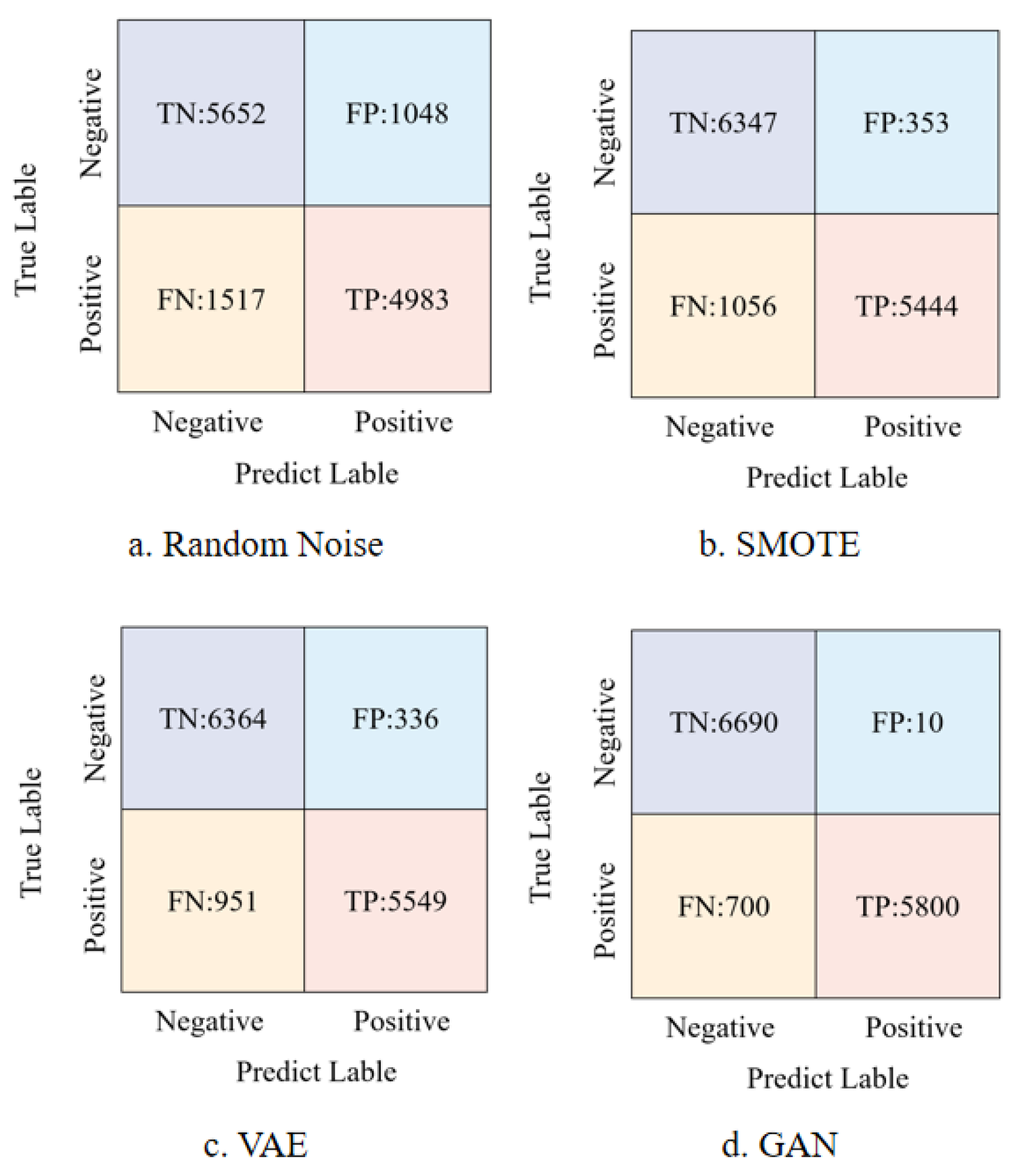
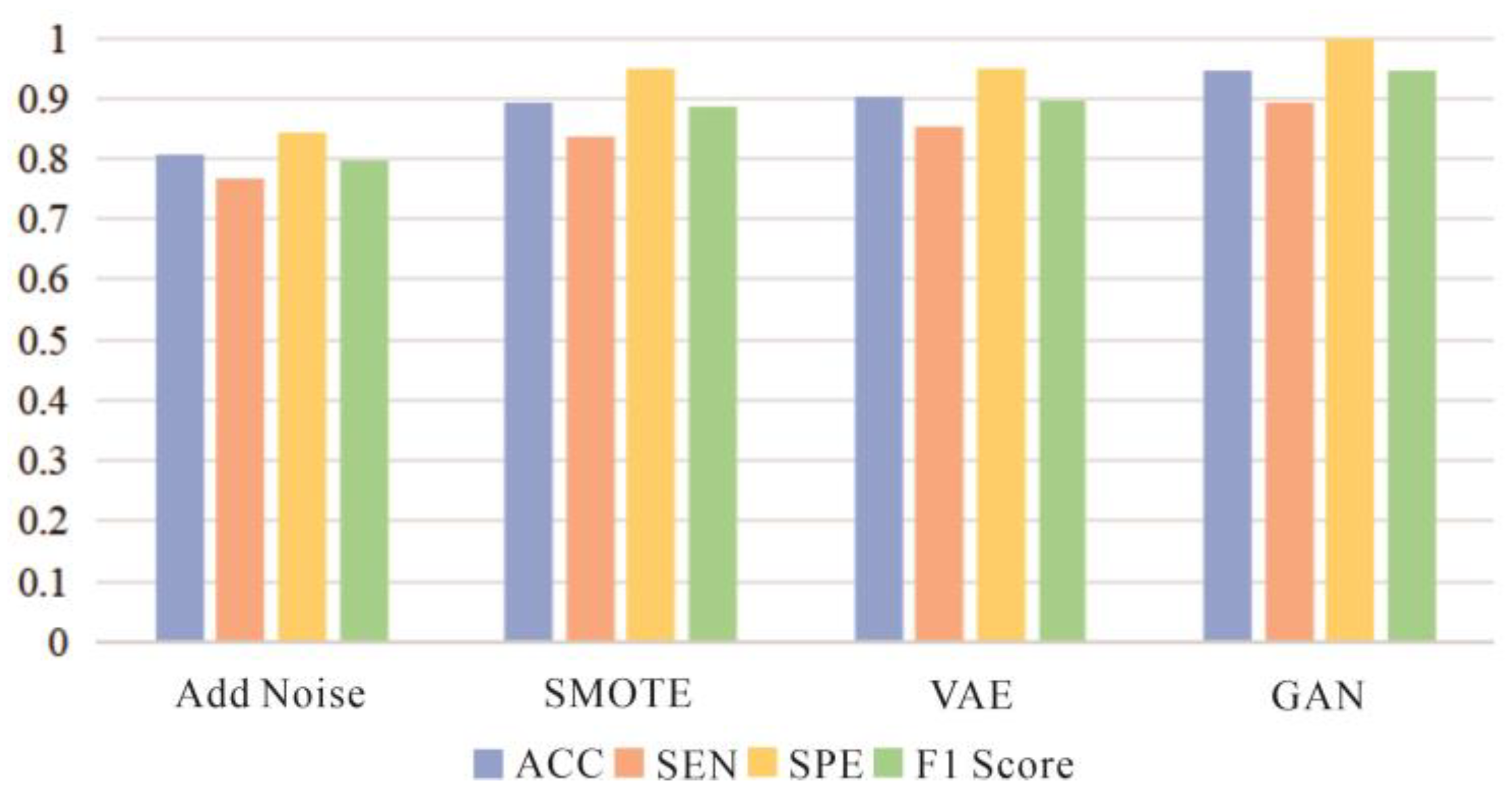
Before model training, this study conducted comparative experiments using four data augmentation methods to improve the model’s generalization ability and prediction accuracy. The specific methods included direct noise addition, SMOTE [40], VAE [41], and GAN. The confusion matrices and comparative experimental results are shown in Figure 11 and Figure 12, respectively.

The following conclusions can be drawn from the performance comparison analysis:

(1)

Direct Noise Addition: Although simple to implement, experimental results show that while this method could identify some mineral deposit samples, it significantly increased the misclassification risk of non-deposit samples, leading to a high number of false positives (FPs) and interfering with the model’s classification ability.

(2)

SMOTE: As a classic technique for handling imbalanced datasets, SMOTE effectively reduced the number of false positives in this experiment, demonstrating its advantage in minimizing non-deposit sample misclassifications. However, the relatively high number of false negatives (FNs) indicates that some actual mineral deposit samples were incorrectly classified as non-deposits, affecting the overall classification performance.

(3)

VAE: The deep learning-based data augmentation method exhibited superior performance by reducing both false positives and false negatives, with significant improvements across all evaluation metrics.

(4)

GAN: The GAN method achieved the best performance across key metrics such as accuracy, sensitivity, specificity, and F1-score. By generating new samples that closely mimic the original data distribution, GAN effectively expanded the dataset size and enhanced the model’s generalization ability, enabling more precise classification of mineral deposits and non-deposits.

In addition, in the labeled data augmentation of geological images, this study positioned known ore deposits as training sample points through manual annotation by professionals. Since mineralization points usually occupied only a few pixels in the image, the study used buffer expansion technology to mark pixels within a certain range around them as “potential mineralization areas”, thus effectively expanding the spatial coverage of training samples. In image convolution operations, the receptive field of the convolution kernel essentially constitutes a spatial buffering mechanism. Specifically, this study generated circular buffers with a preset distance of 50 m centered on the labeled points, realizing the organic integration of geological features and deep learning spatial modeling.

In summary, the experimental results indicate that GAN is the most suitable data augmentation method for this MPM task. It significantly improved the model’s classification performance, reduced misclassification risks, and provided a more reliable solution for MPM.

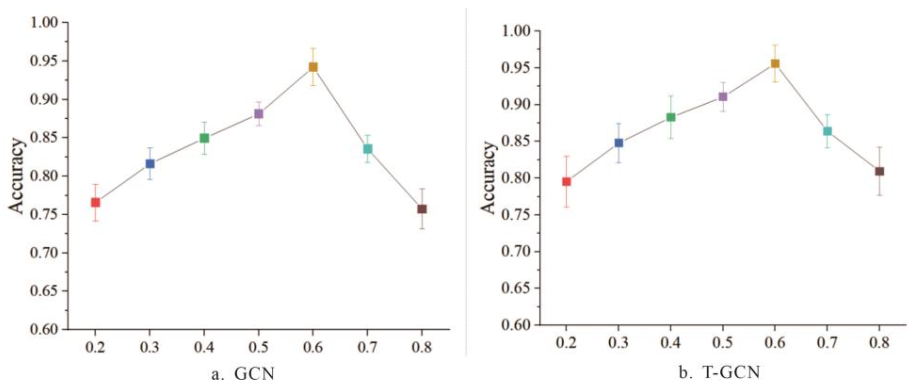
4.3. Influence of Hyperparameter α on Classification Performance

This study systematically analyzed the mechanism by which hyperparameter α affects classification performance. As a threshold for determining the significance of element correlations, α operates through the following process: First, the Pearson correlation coefficient between elements is calculated. If the absolute value of the correlation coefficient exceeds α, a significant correlation is determined between the two elements, and an edge is added to the graph’s adjacency matrix to characterize this association; otherwise, no edge is created. This mechanism indicates that the selection of α directly determines the topological structure of the adjacency matrix, thereby influencing the input features and classification results of the graph neural network.

The study tested the classification ACC of α within the range of {0.2, 0.3, 0.4, 0.5, 0.6, 0.7, 0.8}, with results shown in Figure 13. When α = 0.6, both the GCN and T-GCN models achieved optimal performance in the classification task. This phenomenon can be explained as follows: This threshold retains the key correlations between geochemical elements while filtering out redundant noise, achieving the best balance between information richness and feature purity in the graph structure. The experimental results demonstrate that reasonable selection of α could effectively improve classification accuracy, verifying the importance of this parameter in optimizing the topological modeling of graph neural networks.

4.4. Comparative Experiment with GCNs and Transformer

A comparative experiment was conducted to assess the performance of the T-GCN model in comparison to Transformer and GCNs. The performance metrics under consideration included Acc, sensitivity (Sen), specificity (Spe), and F1 scores.

Table 3. Comparison of GCNs, Transformer, and T-GCN.

Model		1	2	3	4	5	6	7	8	9	10	Average
GCNs	Acc	94.78	94.90	94.99	93.38	93.52	94.72	94.15	94.26	94.32	95.49	94.45
	Sen	87.93	87.81	88.51	84.55	85.07	88.06	86.40	86.85	87.38	89.39	87.2
	Spe	99.91	99.91	99.91	99.93	99.91	99.86	99.93	99.82	99.88	99.89	99.9
	F1	93.52	93.45	93.84	91.58	91.87	93.55	92.66	92.88	93.18	94.59	93.11
Transformer	Acc	95.06	94.68	95.18	95.25	94.61	95.19	95.46	94.85	95.27	95.06	95.03
	Sen	90.67	89.54	91.84	90.94	89.63	91.32	91.01	90.86	91.57	90.67	90.69
	Spe	98.99	99.83	97.79	99.19	98.89	99.58	98.91	98.27	97.98	98.99	98.76
	F1	94.33	93.41	94.43	93.92	94.23	94.91	94.42	94.75	94.71	94.33	94.32
T-GCN	Acc	97.50	97.04	96.44	97.09	97.53	98.04	97.85	96.94	97.44	97.50	97.27
	Sen	92.41	91.93	91.21	92.14	92.38	92.72	92.62	91.78	92.29	92.41	92.15
	Spe	99.93	99.89	99.87	99.91	99.94	99.89	99.95	99.90	99.94	99.93	99.9
	F1	95.91	95.33	94.87	95.64	95.96	96.23	96.07	94.95	95.89	95.91	95.65

lists the accuracy values of GCNs, Transformer, and T-GCN. The results show that T-GCN achieved the highest accuracy of 97.27%, outperforming GCNs (94.45%) and Transformer (95.03%). These data indicate that T-GCN demonstrated superior testing capabilities in precise evaluation of mineral prospectivity.

Figure 14 compares the key performance indicators (Acc, Sen, Spe, and F1-score) of the three models. The results show that:

(1)

Overall Classification Task Performance

T-GCN achieved a higher correct prediction rate in the overall classification task. Its advantages derive from its unique model design, which integrates the global perception capability of Transformer and the graph structure modeling capability of GCNs. This enables the model to comprehensively capture key features in the geochemical element network.

(2)

Sen

T-GCN had a particularly outstanding performance in terms of sensitivity. As a core indicator for measuring the model’s ability to identify positive samples (mineral areas), T-GCN’s high sensitivity means it can effectively reduce the missed detection rate and accurately identify ore-bearing samples.

(3)

Spe

T-GCN and GCNs slightly outperformed Transformer in specificity, indicating that both have more advantages in correctly identifying negative samples (non-mineral areas) and reducing false alarm rates.

(4)

F1 Score

Additionally, T-GCN had the best F1 score (an indicator that integrates precision and recall), demonstrating its excellent performance in balancing the classification accuracy of positive and negative samples.

In summary, T-GCN’s hybrid architecture successfully combines global contextual understanding with local graph structure reasoning, making it superior in both positive sample identification and overall classification balance for mineral prospectivity evaluation.

The above results fully validate the effectiveness of the T-GCN model in mineral prospectivity prediction. Compared with GCNs alone or Transformer, its prediction results are more accurate and reliable. However, the study also finds that the model performance is still constrained by potential challenges such as the quality of graph structure construction. Future research can focus on optimizing the graph modeling process by improving preprocessing techniques and integrating geological prior knowledge to further enhance model performance.

4.5. Comparative Experiments of Different Models

To validate the effectiveness and generalization ability of the T-GCN model, this study selected eight mainstream benchmark models in the classification field for comparative analysis and conducted experiments on three publicly available representative graph datasets (NCII, MUTAG, and IMB-BINARY) and the PangXD dataset. Through multi-dimensional and multi-dataset comprehensive evaluations, a fair performance comparison between T-GCN and other advanced models was achieved. The classification accuracy results are shown in

Table 4. Classification accuracy of different models.

Model	NCII	MUTAG	IMB-BINARY	PangXD
SVM [23]	73.61	71.26	70.25	74.2
Random forest [22]	72.55	71.55	69.92	73.26
K-means [24]	74.56	76.22	75.45	78.03
KNN [22]	73.20	75.10	76.12	77.32
GIN [42]	76.52	82.67	84.22	91.61
SAGPool [43]	73.82	81.49	80.72	93.38
DiffPool [44]	75.74	80.99	87.26	92.25
GraphSAGE [45]	72.98	84.63	86.34	93.51
T-GCN	80.41	82.98	89.63	97.27

.

As shown in Table 3, the T-GCN model demonstrated high classification accuracy across different datasets:

NCII Dataset: T-GCN achieved a classification accuracy of 80.41%, significantly outperforming models such as SVM (73.61%), random forest (72.55%), K-means (74.56%), KNN (73.20%), GIN (76.52%), SAGPool (73.82%), DiffPool (75.74%), and GraphSAGE (72.98%). This indicates its effectiveness in capturing key graph structure information for complex biomolecular graph classification tasks.

MUTAG Dataset: Although T-GCN’s classification accuracy (82.98%) was slightly lower than that of GraphSAGE (84.63%), it remained competitive compared to other models, and the gap fell within a reasonable fluctuation range, verifying the model’s generalization stability.

IMB-BINARY Dataset: T-GCN surpassed all comparative models, with an accuracy of 89.63%, with the second-best model, DiffPool, achieving 87.26%. This further demonstrates its strong capability to handle graph data of different scales and characteristics.

PangXD Dataset: T-GCN achieved an exceptionally high accuracy of 97.27%, significantly outperforming other models. This not only highlights its application advantages in specific fields (e.g., mineral prediction) but also further validates its generalization ability and practical application value.

4.6. Visualization Experiment

This study visualized high-density mineralization areas to accurately locate prospective ore zones. The model constructed based on spatial graph structures effectively revealed key spatial association patterns in mineral prospecting prediction. It accurately reflected the mineralization probability of the target area, efficiently identified potential resource enrichment zones, and strongly supported the reliability of mineral prediction.

In the mineral prospectivity mapping test, the T-GCN model integrating Transformer and graph convolutional operations generated a prospectivity map (Figure 15) that achieved global visualization of mineral potential in the study area. The model demonstrated excellent performance in delineating key mineralization zones, enabling precise capture of high-potential geological features. The high consistency between prediction results and actual mineralized bodies verifies the effectiveness of the model in identifying potential mineral areas. The five prospective targets delineated in this study achieved 100% spatial coverage of known ore deposits in the study area. Comprehensive geological condition analysis showed that each target possesses typical combinations of metallogenic geological factors, making them priority ore deposit prediction targets for follow-up in-depth research.

Through the visualization analysis of the MPM in this study, the fault–mineralization characteristics of five mineral target areas were systematically sorted out. The specific results are shown in

Table 5. The fault–mineralization characteristics of 5 mineral target areas.

Target Number	Fault Structure Characteristics	Element Anomaly and Deposit Distribution
I	Development of deep NE-trending faults with densely distributed secondary faults	Element anomalies distributed in strips along the faults, hosting known large ore deposits
II	Low fault density	Sparsely distributed high-value element anomalies, containing five known ore deposits
III	Conjugate intersection of NE-trending and NW-trending faults with extremely high fault density	Significant element anomaly intensity; no proven ore deposits discovered yet
IV	Densely distributed NW-trending secondary faults	High element anomaly values distributed in a planar manner, with known ore deposits
V	Development of major NE-trending faults with densely developed associated secondary faults	Element anomalies continuously distributed along the fault zone, with known ore deposits

:

Based on the statistical data in Table 5 and combined with the regional geological background, the interpretation of the relationship between fault structures and mineralization in each target area is as follows:

Target I: Located in the northwest of the study area, the deep NE-trending fault serves as the dominant channel for ore fluid migration, while the secondary fault system provides favorable ore storage space. According to the distribution characteristics of element anomalies, it is speculated that this target area is a hydrothermal mineralization zone, with potential ore bodies occurring in layered and vein-like structures along the fault zone, exhibiting high exploration potential.

Target II: This target area is situated in the central part of the study area, where the development of large-scale fault structures is relatively low but small fault structures are commonly developed around the known ore deposits. Considering the occurrence characteristics of the ore deposits, it is inferred that the mineralization may be related to sedimentary environment transformation or magmatic hydrothermal superposition, with relatively weak control of fault structures on mineralization.

Target III: Situated in the southern sector of the study area, this target zone exhibits remarkable element anomaly intensities despite the absence of proven ore deposits. The conjugate intersection of NE-trending and NW-trending faults has formed complex fault–breccia zones, creating ideal structural conduits for ore fluid accumulation. The high spatial coincidence between element anomaly distributions and fault–breccia zones signifies substantial mineralization potential, particularly in fracture intersection areas that serve as preferential sites for hydrothermal ore deposition.

Target IV: Located in the southeastern domain, this target area is characterized by multiphase tectonic activity in fault zones, which has generated abundant dilation zones. A strong positive correlation is observed between element enrichment and fault-related hydrothermal activities, with high-value anomalies distributed in planar patterns controlled by dense NW-trending secondary faults. Comprehensive analysis identifies this zone as a favorable prospect for vein-type deposits, especially where fault networks overlap with lithological contact zones.

Target V: Positioned in the southeastern sector, this target area harbors known ore deposits and features multiphase fault activity that has created extensive dilation zones. Elemental enrichment shows a close genetic link to fault-hosted hydrothermal systems, with anomalies continuously distributed along major NE-trending fault zones. This target is predicted as a prime prospect for vein-type mineralization, supported by the structural control of multiphase faulting on ore body emplacement.

5. Conclusions

This paper proposes a novel T-GCN model for MPM, which significantly enhances the prediction accuracy and interpretability of ore deposit assessments. By fusing Transformer and graph convolutional operations, the model efficiently captures geological features. Cross-model and multi-dataset comparative experiments show that T-GCN outperforms traditional methods in key indicators, including accuracy, sensitivity, specificity, and F1 scores, with a maximum accuracy of 97.27%, demonstrating excellent generalization ability and performance advantages. Visualization experiments further validate its geological interpretation capability, as the prediction results highly coincide with prior geological knowledge and accurately identify high-potential prospecting areas. Studies have revealed significant differences in the analysis efficiency of graph convolutional networks between newly predicted deposits and known operational deposits. The latter allows rapid model training due to massive amounts of accumulated data, while newly predicted deposits require in-depth optimization of model parameters due to data scarcity and complex geological conditions, leading to a substantial extension of the analysis cycle. Constrained by current exploration technologies and data acquisition costs, this study primarily relies on geochemical data and known ore deposit samples within the study area. Future research can be expanded in two aspects: first, introducing transfer learning into geological remote sensing image analysis to reduce over-reliance on local data, and second, integrating metallogenic marker data such as fault structures and lithological contact zones based on existing geochemical analysis to construct a predictive model for multi-source geoscientific data fusion.

References

1. Singer, D.A. Comparison of expert estimates of number of undiscovered mineral deposits with mineral deposit densities. Ore Geol. Rev. 2018, 99, 235–243. [Google Scholar] [CrossRef]
2. Lederer, G.W.; Solano, F.; Coyan, J.A.; Denton, K.M.; Watts, K.E.; Mercer, C.N.; Bickerstaff, D.P.; Granitto, M. Tungsten skarn mineral resource assessment of the great basin region of western Nevada and eastern California. J. Geochem. Explor. 2021, 223, 106712. [Google Scholar] [CrossRef]
3. Jo, J.; Lee, B.H.; Heo, C.H. Geochemical approaches to mineral resources exploration. Econ. Environ. Geol. 2024, 57, 593–608. [Google Scholar] [CrossRef]
4. Coyan, J.; Solano, F.; Taylor, C.; Finn, C.; Smith, S.; Holm-Denoma, C.; Pianowski, L.; Crocker, K.; Mirkamalov, R.; Divaev, F. Tungsten skarn quantitative mineral resource assessment and gold, rare earth elements, graphite, and uranium qualitative assessments of the kuldjuktau and auminzatau ranges, in the central kyzylkum region, Uzbekistan. Minerals 2024, 14, 1240. [Google Scholar] [CrossRef]
5. Partington, G.A.; Peters, K.J.; Czertowicz, T.A.; Greville, P.A.; Blevin, P.L.; Bahiru, E.A. Ranking mineral exploration targets in support of commercial decision making: A key component for inclusion in an exploration information system. Appl. Geochem. 2024, 168, 106010. [Google Scholar] [CrossRef]
6. Ding, M.; Vatsalan, D.; Gonzalez-Alvarez, I.; Mrabet, S.; Tyler, P.; Klump, J. Trusted data sharing for mineral exploration and mining tenements. J. Geochem. Explor. 2024, 267, 107580. [Google Scholar] [CrossRef]
7. Liu, F.M. Enabling data conversion between Micromine and Surpac- enhancing efficiency in geological exploration. Cogent Educ. 2024, 11, 2438591. [Google Scholar] [CrossRef]
8. Huang, J.; Fang, Y.; Wang, C.; Li, Y. Research on 3D geological and numerical unified model of in mining slope based on multi-source data. Water 2024, 16, 2421. [Google Scholar] [CrossRef]
9. Jin, X.; Wang, G.W.; Tang, P.; Zhang, S.K. 3D geological modelling and uncertainty analysis for 3D targeting in Shanggong gold deposit (China). J. Geochem. Explor. 2020, 210, 106442. [Google Scholar] [CrossRef]
10. Cai, H.H.; Chen, S.Q.; Xu, Y.Y.; Li, Z.X.; Ran, X.J.; Wen, X.P. Intelligent recognition of ore-forming anomalies based on multisource data fusion: A case study of the Daqiao mining area, Gansu province, China. Earth Space Sci. 2021, 8, e2021EA001927. [Google Scholar] [CrossRef]
11. Zuo, R.G.; Yang, F.F.; Cheng, Q.M.; Kreuzer, O.P. A novel data-knowledge dual-driven model coupling artificial intelligence with a mineral systems approach for mineral prospectivity mapping. Geology 2025, 53, 284–288. [Google Scholar] [CrossRef]
12. He, L.H.; Zhou, Y.Z.; Zhang, C. Application of target detection based on deep learning in intelligent mineral identification. Minerals 2024, 14, 873. [Google Scholar] [CrossRef]
13. Yang, L.; Liu, M.; Liu, N.; Guo, J.Y.; Lin, L.A.; Zhang, Y.Y.; Du, X.; Wang, Y.K. Recovering bathymetry from satellite altimetry-derived gravity by fully connected deep neural network. IEEE Geosci. Remote Sens. Lett. 2023, 20, 1502805. [Google Scholar] [CrossRef]
14. Zhang, Z.H.; Wang, Y.B.; Wang, P. On a deep learning method of estimating reservoir porosity. Math. Probl. Eng. 2021, 2021, 6641678. [Google Scholar] [CrossRef]
15. Saremi, M.; Bagheri, M.; Mirzabozorg, S.; Hassan, N.E.; Hoseinzade, Z.; Maghsoudi, A.; Rezania, S.; Pour, A.B. Evaluation of deep isolation forest(DIF) algorithm for mineral prospectivity mapping of polymetallic deposits. Minerals 2024, 14, 1015. [Google Scholar] [CrossRef]
16. Chen, M.M.; Xiao, F. Projection pursuit random forest for mineral prospectivity mapping. Math. Geosci. 2023, 55, 963–987. [Google Scholar] [CrossRef]
17. Gao, L.; Zhang, W.T.; Liu, Q.Y.; Zhang, X. Machine learning based on the graph convolutional self-organizing map method increases the accuracy of pollution source identification: A case study of trace metal(loid)s in soils of Jiangmen City, south China. Ecotoxicol. Environ. Saf. 2023, 250, 114467. [Google Scholar] [CrossRef]
18. Zuo, R.G.; Carranza, E.J.M. Support vector machine: A tool for mapping mineral prospectivity. Comput. Geosci. 2011, 37, 1967–1975. [Google Scholar] [CrossRef]
19. Maepa, F.; Smith, R.S.; Tessema, A. Support vector machine and artificial neural network modelling of orogenic gold prospectivity mapping in the Swayze greenstone belt, Ontario, Canada. Ore Geol. Rev. 2021, 130, 103968. [Google Scholar] [CrossRef]
20. Behnia, P.; Harris, J.; Sherlock, R.; Naghizadeh, M.; Vayavur, R. Mineral prospectivity mapping for orogenic gold mineralization in the rainy river area, Wabigoon subprovince. Minerals 2023, 13, 1267. [Google Scholar] [CrossRef]
21. Cao, C.J.; Wang, X.L.; Yang, F.; Xie, M.; Liu, B.; Zhou, Z.L. Attention-driven graph convolutional neural networks for mineral prospectivity mapping. Ore Geol. Rev. 2025, 180, 106554. [Google Scholar] [CrossRef]
22. Cao, M.X.; Yin, D.M.; Zhong, Y.; Lv, Y. Detection of geochemical anomalies related to mineralization using the random forest model optimized by the competitive mechanism and beetle antennae search. J. Geochem. Explor. 2023, 249, 107195. [Google Scholar] [CrossRef]
23. Lachaud, A.; Adam, M.; Miskovic, I. Comparative study of random forest and support vector machine algorithms in mineral prospectivity mapping with limited training data. Minerals 2023, 13, 1073. [Google Scholar] [CrossRef]
24. Ghezelbash, R.; Maghsoudi, A.; Shamekhi, M. Genetic algorithm to optimize the SVM and K-means algorithms for mapping of mineral prospectivity. Neural Comput. Appl. 2023, 35, 719–733. [Google Scholar] [CrossRef]
25. Shaw, K.O.; Goita, K.; Germain, M. Prospectivity mapping of heavy mineral ore deposits based upon machine-learning algorithms: Columbite-tantalite deposits in west-central cote d’lvoire. Minerals 2022, 12, 1453. [Google Scholar] [CrossRef]
26. Xiao, F.; Chen, W.L.; Erten, Q. A hybrid logistic regression: Gene expression programming model and its application to mineral prospectivity mapping. Nat. Resour. Res. 2022, 31, 2041–2064. [Google Scholar] [CrossRef]
27. Li, H.; Li, X.h.; Yuan, F.; Jowitt, S.M.; Wu, B.C. Convolutional neural network and transfer learning based mineral prospectivity modeling for geochemical exploration of Au mineralization within the Guandian-Zhangbaling area, Anhui Province, China. Appl. Geochem. 2020, 122, 104747. [Google Scholar] [CrossRef]
28. Gao, L.; Huang, Y.J.; Zhang, X.; Liu, Q.Y.; Chen, Z.Q. Prediction of prospecting target based on resnet convolutional neural network. Appl. Sci. 2022, 12, 11433. [Google Scholar] [CrossRef]
29. Huang, Y.; Feng, Q.; Zhang, W.; Zhang, X.; Gao, L. Prediction of prospecting target based on selective transfer network. Minerals 2022, 12, 1112. [Google Scholar] [CrossRef]
30. Xiao, F.; Wang, Y.; Zhou, Y.Z. Determining thresholds of arsenic and mercury in stream sediment for mapping natural toxic element anomaly using data-driven models: A comparative study on probability plots and fractal methods. Arab. J. Geosci. 2020, 13, 9155. [Google Scholar] [CrossRef]
31. Yu, X.T.; Yu, P.; Wang, K.Y.; Cao, W.; Zhou, Y.Z. Data-driven mineral prospectivity mapping based on known deposits using association rules. Nat. Resour. Res. 2024, 33, 1025–1048. [Google Scholar] [CrossRef]
32. Zhou, Y.Z.; Zhang, Q.L.; Huang, Y.J.; Yang, W.; Xiao, F.; Shen, W.J. Constructing knowledge graph for the porphyry copper deposit in the Qinzhou-Hangzhou bay area: Insight into knowledge graph based mineral resource prediction and evaluation. Earth Sci. Front. 2021, 28, 67–75. [Google Scholar] [CrossRef]
33. He, J.X.; Zhang, Q.L.; Xu, Y.; Liu, Y.; Zhou, Y.Z. Research progress ofQinzhou-Hangzhou metallogenic belt- analysed from citespace community discovery. Geol. Rev. 2023, 69, 1919–1927. [Google Scholar] [CrossRef]
34. Salomao, G.N.; Dall’Agnol, R.; Angelica, R.S.; Sahoo, P.K. Geochemical mapping in stream sediments of the Carajás Mineral Province, part 2: Multi-element geochemical signatures using Compositional Data Analysis(CoDA). J. S. Am. Earth Sci. 2021, 110, 103361. [Google Scholar] [CrossRef]
35. Yerke, A.; Brumit, D.F.; Fodor, A.A. Proportion-based normalizations outperform compositional data transformations in machine learning applications. Microbiome 2024, 12, 45. [Google Scholar] [CrossRef] [PubMed]
36. Graffelman, J.; Pawlowsky-Glahn, V.; Egozcue, J.J.; Buccianti, A. Exploration of geochemical data with compositional canonical biplots. J. Geochem. Explor. 2018, 194, 120–133. [Google Scholar] [CrossRef]
37. Cheng, J.R.; Yang, Y.; Tang, X.Y.; Xiong, N.X.; Zhang, Y.; Lei, F.F. Generative adversarial networks: A literature review. KSII Trans. Internet Inf. Syst. 2020, 14, 4625–4647. [Google Scholar] [CrossRef]
38. Nayak, G.H.H.; Alam, M.W.; Avinash, G.; Kumar, R.R.; Ray, M. Transformer-based deep learning architecture for time series forecasting. Softw. Impacts 2024, 22, 100716. [Google Scholar] [CrossRef]
39. Zhou, Y.; Zheng, H.X.; Huang, X.; Hao, S.F.; Li, D.; Zhao, J.M. Graph neural networks: Taxonomy, advances, and trends. ACM Trans. Intell. Syst. Technol. 2022, 13, 15. [Google Scholar] [CrossRef]
40. De Carvalho, A.M.; Prati, R.C. DTO-SMOTE: Delaunay tessellation oversampling for imbalanced data sets. Information 2020, 11, 557. [Google Scholar] [CrossRef]
41. Jagadish, D.N.; Chauhan, A.; Mahto, L.; Chakraborty, T. Autonomous vehicle path prediction using conditional variational autoencoder networks. Adv. Knowl. Discov. Data Min. 2021, 12712, 129–139. [Google Scholar] [CrossRef]
42. Kivela, M.; Porter, M.A. Isomorphisms in multilayer networks. IEEE Trans. Netw. Sci. Eng. 2018, 5, 198–211. [Google Scholar] [CrossRef]
43. Liu, C.; Zhan, Y.B.; Yu, B.S.; Liu, L.; Liu, T.L. Onexploring node-feature and graph-structure diversities for node drop graph pooling. Neural Netw. 2023, 167, 559–571. [Google Scholar] [CrossRef] [PubMed]
44. Pham, H.V.; Thanh, D.H.; Moore, P. Hierarchical pooling in graph neural networks to enhance classification performance in large datasets. Sensors 2021, 21, 6070. [Google Scholar] [CrossRef]
45. Zhang, T.; Shan, H.R.; Little, M.A. Causal graphSAGE: A robust graph method for classification based on causal sampling. Pattern Recognit. 2022, 128, 108696. [Google Scholar] [CrossRef]
Figure 1. The geological background of the PangXD area. (a) Geotectonic location of the PangXD area. (b) Comprehensive geology and deposit distribution map of the PangXD area.
Minerals 15 00711 g001
Figure 2. The spatial distribution of Pb–Zn elements across the study area.
Minerals 15 00711 g002
Figure 3. The network structure diagram of T-GCN.
Minerals 15 00711 g003
Figure 4. Distribution of data before and after transformation. (a) Box plot of raw data; (b) violin plot of log-transformed data; (c) violin plot of CLR-transformed data.
Minerals 15 00711 g004
Figure 5. Density distribution curve after data transformation. (a) Curve after log-transformation; (b) Curve after CLR transformation.
Minerals 15 00711 g005
Figure 6. Schematic architecture of the GAN framework.
Minerals 15 00711 g006
Figure 7. Schematic architecture of the Transformer framework.
Minerals 15 00711 g007
Figure 8. The mechanism structure diagram of self-attention.
Minerals 15 00711 g008
Figure 9. The mechanism structure diagram of multi-head attention.
Minerals 15 00711 g009
Figure 10. The process of feature aggregation.
Minerals 15 00711 g010
Figure 11. Confusion metrices under different augmentation techniques.
Minerals 15 00711 g011
Figure 12. Performance comparison diagram of different augmentation methods.
Minerals 15 00711 g012
Figure 13. Accuracy for different values of α.
Minerals 15 00711 g013
Figure 14. Comparison diagram of model performance experimental results. (a) ACC performance comparison; (b) SEN performance comparison; (c) SPE performance comparison; (d) F1 Score performance comparison.
Minerals 15 00711 g014
Figure 15. The visualization of the mineral prospectivity map using T-GCN.
Minerals 15 00711 g015