Article

Predicting Industrial Copper Hydrometallurgy Output with Deep Learning Approach Using Data Augmentation

by
Bagdaulet Kenzhaliyev
1,
Nurtugan Azatbekuly
2,
Serik Aibagarov
2,*,
Bibars Amangeldy
2,*,
Aigul Koizhanova
1 and
David Magomedov
1
1
Institute of Metallurgy and Ore Beneficiation, Satbayev University, Almaty 050000, Kazakhstan
2
Faculty of Information Technology, Al-Farabi Kazakh National University, Almaty 050000, Kazakhstan
*
Authors to whom correspondence should be addressed.
Minerals 2025, 15(7), 702; https://doi.org/10.3390/min15070702
Submission received: 15 April 2025 / Revised: 16 May 2025 / Accepted: 27 May 2025 / Published: 30 June 2025
(This article belongs to the Section Mineral Processing and Extractive Metallurgy)

Abstract

Sustainable copper extraction presents significant challenges due to waste generation and environmental impacts, requiring advanced predictive methodologies to optimize production processes. This study addresses a gap in applying deep learning to forecast hydrometallurgical copper production by comparing six recurrent neural network architectures: Vanilla LSTM, Stacked LSTM, Bidirectional LSTM, GRU, CNN-LSTM, and Attention LSTM. Using time-series data from a full-scale industrial operation, we implemented a data augmentation approach to overcome data scarcity limitations. The models were evaluated through rigorous metrics and multi-step forecasting tests. The results demonstrated remarkable performance from five architectures, with Bidirectional LSTM and Attention LSTM achieving the highest accuracy (RMSE < 0.004, R2 > 0.999, MAPE < 1%). These models successfully captured and reproduced complex cyclical patterns in copper mass production for up to 500 time steps ahead. The findings validate our data augmentation strategy for enabling models to learn complex known cyclical patterns from limited initial data and establish a promising foundation for implementing AI-driven predictive systems that can enhance process control, reduce waste, and advance sustainability in hydrometallurgical operations. However, these performance metrics reflect the models’ ability to reproduce patterns inherent in the augmented dataset derived from a single operational cycle; validation on entirely independent operational data is crucial for assessing true generalization and is a critical next step.

1. Introduction

Growing global demand for copper has spurred large-scale resource extraction that, however, generates significant waste streams and environmental challenges. The extraction process produces vast amounts of smelter slag, acid sludge, industrial dust, and hazardous residues from end-of-life electronics, all of which complicate waste management and pose serious environmental risks [1,2,3,4,5]. Complex feedstocks such as chalcopyrite ores and low-grade materials further exacerbate these issues, leading to high reagent consumption and inefficient energy use [6,7]. Conventional processes often rely on environmentally detrimental reagents, while the handling of acid sludge and industrial by-products can result in the release of toxic elements into ecosystems [8,9,10]. These problems underscore the need for more sustainable methods of metal extraction that can simultaneously reduce waste, lower energy requirements, and protect the environment.
In response, hydrometallurgy has emerged as a promising framework to improve copper recovery while mitigating waste and environmental impacts. Researchers have developed specialized software to automate hydrometallurgical calculations and optimize process efficiency, enabling more accurate control over multi-stage extraction operations [11]. Innovative techniques such as ultrasound-assisted leaching have been compared with conventional methods to enhance metal dissolution and recovery rates [12], while dynamic acid leaching systems for printed circuit boards demonstrate promising results in achieving high copper solubilization [13]. Advances in hydrometallurgical processing are further evidenced by studies that focus on waste valorization, such as the recovery of copper from slag and anode furnace dust [14], and on the use of alternative reagents derived from mill scale [15]. The implementation of circular hydrometallurgy principles has led to novel frameworks for reagent regeneration, water recycling, and waste minimization, forming a benchmark for sustainable process design [16]. Alternative water sources, including the use of seawater in Chilean copper mining, offer potential benefits despite introducing challenges related to high salinity and corrosion [17]. In parallel, advanced modeling techniques, such as Gaussian process regression and hybrid genetic algorithms, have been applied to optimize leaching kinetics and process conditions [18,19,20]. Optimized bioengineered copper recovery from e-waste further demonstrates the feasibility of environmentally friendly extraction methods [21], while comprehensive reviews of chalcopyrite leaching techniques provide critical insights into overcoming passivation and kinetic limitations [22]. Additional research efforts have also addressed recovery from complex industrial wastes, such as hydrometallurgical approaches for copper-rich side streams [23], reactor and column leaching studies [24], recovery from shredded ICT products [25], and state-of-the-art process control methodologies [26]. Other studies, including detailed comparisons of deep eutectic solvents, have broadened our understanding of alternative green reagents in metal recovery [27].
Complementing these chemical and process innovations is a growing integration of artificial intelligence and neural network methodologies into hydrometallurgical systems. Machine learning has proven invaluable in modeling mineral leaching processes, offering enhanced predictive capabilities that help optimize operational parameters [28]. AI-driven decision support systems are now being developed to guide complex process adjustments and facilitate real-time control, thereby improving recovery rates and reducing waste [29]. Comparative studies using supervised learning algorithms have demonstrated that random forest models and artificial neural networks can accurately predict copper recovery quality, thereby refining process control strategies [30]. Furthermore, recurrent neural networks with attention mechanisms have been successfully applied to forecast cathode rejection during the electrorefining stage, ensuring timely adjustments to maintain high product purity [31]. Advanced neural network architectures have also been implemented to target selective impurity removal in challenging feedstocks, such as flash furnace electrostatic precipitator dust [32], and feed-forward ANNs have optimized copper and cobalt recovery from oxide ores with remarkable precision [33]. Broader reviews of current copper ore processing techniques illustrate how digital transformation is reshaping operational workflows and equipment design [34], while bibliometric analyses of hydrometallurgy research reveal emerging hotspots and the increasing role of AI in process innovation [35]. Other studies employing random forest models have further underscored the potential of AI to enhance leaching efficiency [36], and stochastic modeling approaches based on Bayesian networks offer robust frameworks for handling process uncertainties in copper heap leaching [37].
While existing research showcases the increasing integration of AI into hydrometallurgy for process enhancement, a significant research gap remains in the effective application of advanced deep learning methodologies for comprehensive, predictive modeling of overall copper production in real-world industrial settings. Current studies often focus on specific process stages or utilize simplified datasets, leaving a critical need to address the challenges of limited real-world industrial data and the complex, dynamic nature of full-scale hydrometallurgical operations. Therefore, this study tackles the crucial problem of accurately and reliably forecasting key performance indicators of copper production, specifically total copper mass, in a full-scale hydrometallurgical extraction process, with an initial focus on leveraging data augmentation to overcome severe data limitations and assess the capability of various deep learning models to learn and reproduce the inherent complex cyclical dynamics from such augmented data.
To address this challenge, our research explores and compares the efficacy of several advanced deep learning architectures for time-series forecasting, including Vanilla LSTM, Stacked LSTM, Bidirectional LSTM, GRU, CNN-LSTM, and Attention LSTM. Trained on real-world industrial data, augmented to overcome data limitations, this work aims to demonstrate the practical feasibility and accuracy of deep learning for predicting key production metrics in an operational industrial environment. Furthermore, it provides a comparative analysis of these diverse deep learning approaches for copper extraction forecasting, validates a data augmentation strategy to mitigate data scarcity, and ultimately highlights the potential of AI-driven predictive models to significantly advance process understanding, optimization efforts, and the pursuit of more sustainable practices within the field of copper hydrometallurgy.

2. Hydrometallurgical Copper Extraction Process

Hydrometallurgical methods enable the extraction of copper and other valuable elements from mineral raw materials through chemical reactions in aqueous solutions. The process typically includes leaching, extraction, re-extraction, and electrolysis. During leaching, sulfuric acid dissolves copper from crushed ore, forming a productive solution. This solution is then treated with an organic extractant that selectively binds copper ions, enriching the metal content while allowing the raffinate to be reused. In the re-extraction phase, copper is transferred from the organic phase back into an aqueous solution, creating a concentrated electrolyte. Finally, electrolysis is used to deposit pure copper onto cathodes, while the remaining solution continuously recirculates through the system.
In full-scale operations, the total duration of the hydrometallurgical process can vary widely based on factors like ore composition, operational scale, and climate conditions. In the example described here, we use a 150-day cycle. Over approximately the first 60 days, leaching dominates as sulfuric acid percolates through large heaps or lined ponds, gradually dissolving copper into solutions. Once enough copper accumulates in the productive solution, extraction and re-extraction typically proceed for about 30 days, during which organic extractants selectively bind copper ions and transfer them into a more concentrated aqueous electrolyte. The final 60 days complete the process via electrolysis, where the copper-rich electrolyte flows into electrolysis cells and pure metal is deposited onto cathodes before being recirculated.
Throughout this 150-day cycle, flow rates, acid concentrations, and temperature are monitored daily to maintain optimal leaching efficiency, while on-site laboratories analyze key samples—such as raffinate, loaded organic, and rich electrolyte—to make real-time adjustments. Such integrated control allows operators to adapt to seasonal variations, differences in ore composition, and changing reagent requirements, ensuring that each stage consistently achieves high copper recovery.

3. Materials and Methods

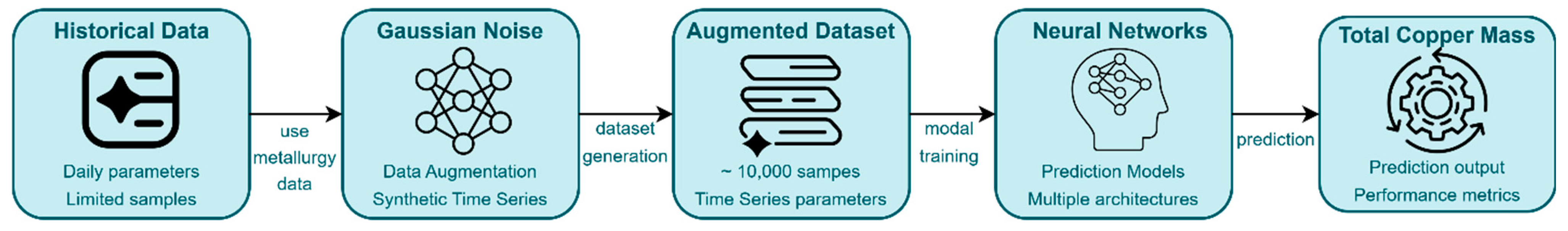
3.1. Study Overview and Experimental Design

Figure 1 illustrates the complete workflow of our approach to copper production forecasting. The process begins with limited historical data containing daily operational parameters from copper extraction operations. These data undergo augmentation through the application of Gaussian noise to generate a synthetic time series, resulting in an expanded dataset of approximately 10,000 samples. The augmented dataset is then used to train multiple neural network architectures, which are evaluated for their ability to accurately predict total copper mass under various conditions.

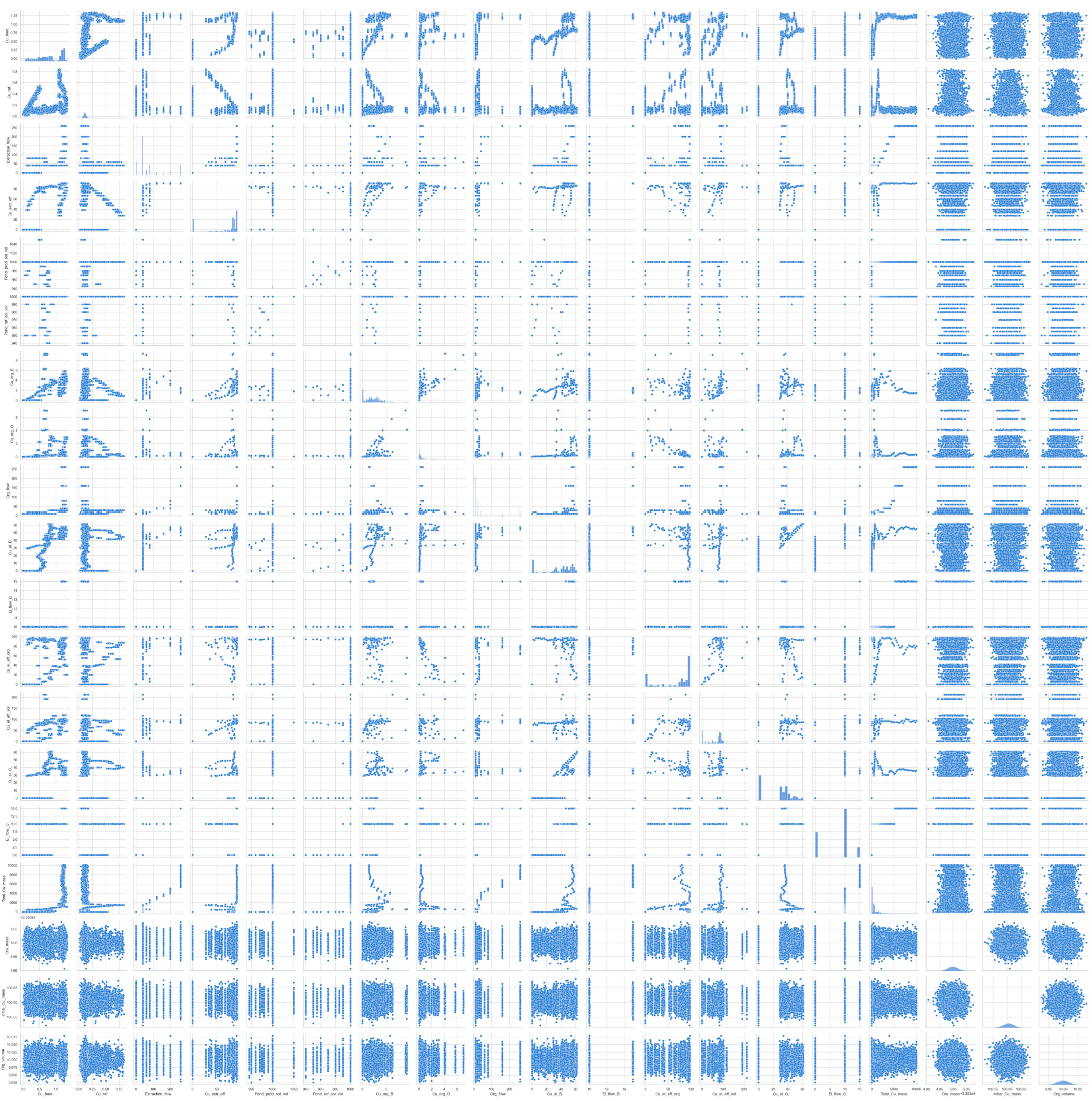
3.2. Data Collection and Preparation

The dataset was constructed from an organized set of industrial field trials supported by specific laboratory investigations, encompassing continuous on-site monitoring and scheduled sampling. Because it was gathered directly under real-world, full-scale operational conditions, our data provide a more robust and accurate perspective on copper recovery compared to previous data used in [11]. It integrates time-based tracking of concentration changes, dynamic flow parameters, and real-time laboratory and field data, further enhanced by automated error-checking routines and direct links between key performance indicators and batch-specific parameters. These measures ensured the completeness and reliability of the initial 150-day dataset, which did not contain missing values or obvious unhandled outliers requiring specific imputation or exclusion prior to augmentation.
The initial dataset comprised observational data collected over a single 150-day operational cycle. This dataset contained time-series measurements of 22 process variables, including the target variable of interest: total copper mass. Table 1 presents the complete list of measured variables, their measurement types, and descriptions of their role in the hydrometallurgical copper extraction process.
Given the limited duration of the original data, a data augmentation strategy was employed to generate a larger, synthetic dataset suitable for training deep learning models while preserving the underlying temporal dynamics observed in the original cycle.

3.3. Data Preprocessing and Feature Engineering

3.3.1. Data Augmentation

Synthetic data [38,39] generation involved creating 10,000 simulated 150-day cycles (approx. 66 full cycles). Each synthetic cycle was based on the original 150-day sequence. To introduce the variability characteristic of real-world processes, Gaussian noise was added independently to each non-zero data point within a copied cycle. The noise followed a normal distribution with a mean of 0 and a standard deviation of 0.02. The mean of 0 ensured that the noise introduced did not systematically bias the signal upward or downward, thus preserving the original trend of the data. The standard deviation of 0.02 was selected to reflect a realistic level of variability observed in the original dataset: small enough to maintain the underlying pattern but large enough to simulate the natural fluctuations in the process. While this IID Gaussian noise is a simplification of potentially more complex real-world disturbances (e.g., heteroscedasticity, autocorrelation), it served as a controlled initial method to introduce variability for this feasibility study on learning cyclical patterns from augmented limited data.
Data points originally recorded as zero were kept at zero in the synthetic cycles to maintain sparsity patterns inherent in the process. The augmented cycles were concatenated sequentially, resulting in an expanded time-series dataset containing 9900 time steps. The pairwise relationship between the features can be seen in Appendix A, Figure A1.

3.3.2. Feature Selection and Scaling

Prior to model training, preliminary feature selection was performed. Three features, ‘Ore_to_metal_extr’, ‘Total_extraction_eff’, and ‘Cu_cat_growth’, were removed from the dataset because they reveal information that would not be available in a real-world predictive scenario. These features are calculated after the total copper mass (‘Total_Cu_mass’) is known, effectively giving away information about the target variable. Including them would lead to data leakage and overly optimistic model performance. The remaining 19 features, including the target variable, were then standardized using StandardScaler from the Scikit-learn library.
This process involved calculating the mean and standard deviation for each feature across the entire augmented training dataset partition (as described in Section 3.3.3) and transforming the data such that each feature had a mean of zero and a standard deviation of one. The scaling parameters derived from the training data were subsequently used to transform the validation and test sets, preventing data leakage. For the comparative analysis of different models (Section 3.4.1), separate scalers were fitted on the training features and training target variable, respectively, to ensure target variable scaling was handled independently during evaluation. The final preprocessed data were converted into PyTorch tensors for model input.

3.3.3. Time Series Preparation and Dataset Splitting

To structure the data for sequence modeling, a sliding window approach was implemented. The preprocessed time series was transformed into sequences of fixed length (sequence length = 10). Each input sample (X) consisted of 10 consecutive time steps, encompassing all 19 features. The corresponding target (y) for each input sequence was the ‘Total_Cu_mass’ value (scaled) at the time step immediately following the end of the input sequence (i.e., time step t + 10 given an input sequence from t to t + 9). This resulted in input tensors of shape (9890, 10, 19) and target tensors of shape (9890, 1).
The 10 consecutive time steps represent 10 days of operational data. This window length was chosen based on preliminary assessments to balance capturing recent operational dynamics relevant for next-day forecasting with computational considerations for training multiple architectures. Our experiments with windows of different lengths (5, 10, 15, 20 steps) showed that a 10-step window provides the optimal balance between these factors for this task.
For the comparative evaluation of different recurrent architectures the sequence dataset was split into training, validation, and testing sets. First, 20% of the data was held out as the final test set. The remaining 80% was further divided, allocating 80% for training and 20% for validation. This resulted in an approximate 64% training, 16% validation, and 20% testing split of the total sequence data. The split was performed chronologically before shuffling the training data loader to maintain temporal order for validation and testing.

3.4. Model Development and Evaluation

3.4.1. Model Architectures

To address the challenge of accurate copper production forecasting, our research explores and compares the efficacy of several advanced deep learning architectures for time-series forecasting [40]:
  • Vanilla LSTM—A standard Long Short-Term Memory network with a single LSTM layer and a hidden state dimension of 50.
  • Stacked LSTM—An LSTM network with multiple stacked LSTM layers (num_layers = 3) and a hidden dimension of 50.
  • Bidirectional LSTM (Bi-LSTM)—An LSTM network utilizing a single bidirectional layer, processing the input sequence in both forward and backward directions. The hidden dimension was 50 (resulting in 100 features before the final layer).
  • GRU (Gated Recurrent Unit)—A network using a GRU layer instead of LSTM, with a hidden dimension of 50.
  • CNN-LSTM—A hybrid model combining a 1D Convolutional Neural Network (CNN) layer for feature extraction across the input features at each time step, followed by an LSTM layer. The CNN layer had 32 filters and a kernel size of 3. The subsequent LSTM layer had a hidden dimension of 50.
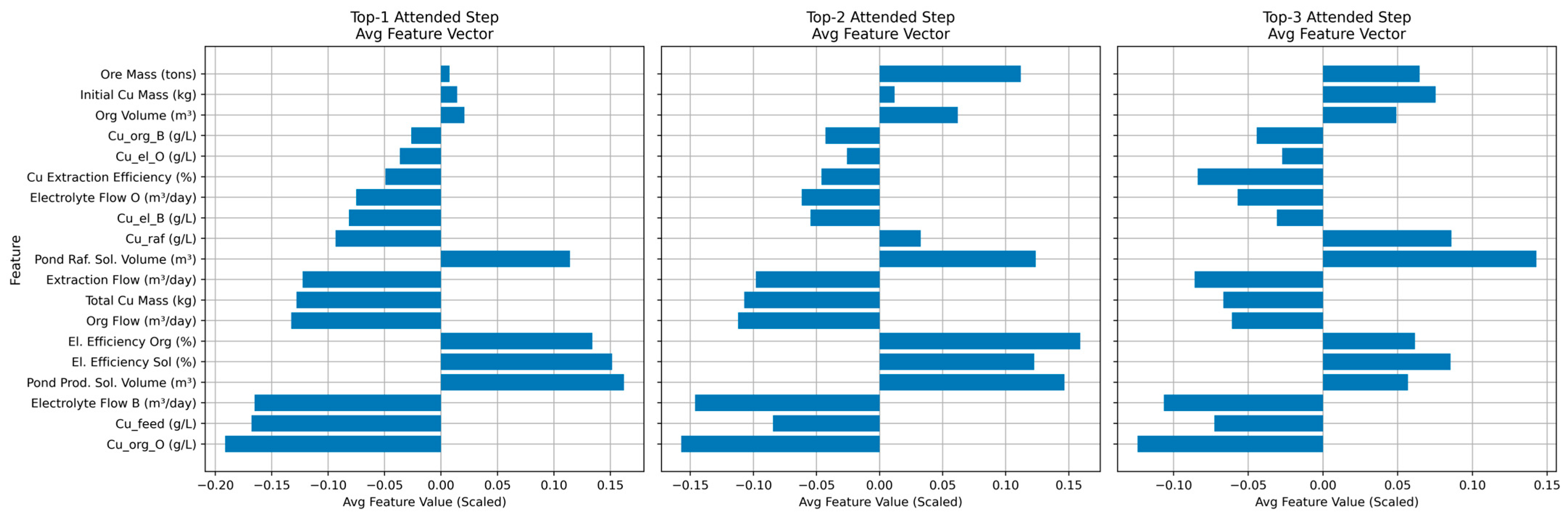
  • Attention LSTM—An LSTM network augmented with a simple attention mechanism. Attention weights were computed over the LSTM output sequence, allowing the model to weigh the importance of different time steps dynamically before producing the final prediction. It used a single LSTM layer with a hidden dimension of 50.
All models utilized a final fully connected (linear) layer to map the hidden state representation from the recurrent or attention layer to a single output value, corresponding to the predicted ‘Total_Cu_mass’.

3.4.2. Training Procedure

All six models were trained using the Adam optimizer with a learning rate of 0.01. The Mean Squared Error (MSE) was employed as the loss function. Training was performed using mini-batches of size 128. The training data loader shuffled the samples at each epoch.
An early stopping mechanism was implemented based on the validation loss. Training proceeded for a maximum of 500 epochs. If the validation loss did not improve for 50 consecutive epochs, training was halted, and the model parameters corresponding to the epoch with the lowest validation loss were retained as the best model state. Training was performed on a CUDA-enabled NVIDIA RTX 4060Ti. Training and validation losses were recorded for each epoch.
A hidden state dimension of 50 was used for the recurrent layers, and a learning rate of 0.01 with the Adam optimizer was employed for all models. These common hyperparameters were kept consistent across architectures to allow for a clearer comparison of their inherent capabilities in processing the augmented time-series data, rather than conducting an exhaustive hyperparameter optimization for each model, which was outside the scope of this initial comparative study. Such optimization would be a focus in subsequent refinement phases for promising candidates.

3.4.3. Evaluation Metrics

The performance of each trained model (using the best state saved via early stopping) was evaluated on the training, validation, and test sets.
  • Mean Absolute Error (MAE): The MAE provides a straightforward interpretation of the average magnitude of errors in the same unit as the target variable. It is robust to outliers and offers an intuitive measure of model accuracy in terms of absolute deviation from true values [38].
  • Root Mean Squared Error (RMSE): The RMSE penalizes larger errors more heavily than MAE due to the squaring operation. This makes it especially useful when larger deviations are more critical to the application, providing a more sensitive error measurement for high-impact mispredictions [38].
  • Coefficient of Determination (R2): R2 indicates the proportion of variance in the target variable that is predictable from the input features. It offers a normalized metric to assess how well the model explains the data, facilitating comparisons across models regardless of the scale of the target variable [38].
  • Mean Absolute Percentage Error (MAPE): The MAPE expresses errors as a percentage of actual values, which is useful for interpretability when comparing performance across datasets or time periods. Since MAPE can become unstable when true values approach zero, care was taken to ensure zero values were appropriately handled or excluded from its calculation [41].
These metrics were chosen to collectively capture multiple aspects of model performance: absolute accuracy (MAE), sensitivity to large errors (RMSE), explanatory power (R2), and relative accuracy (MAPE).

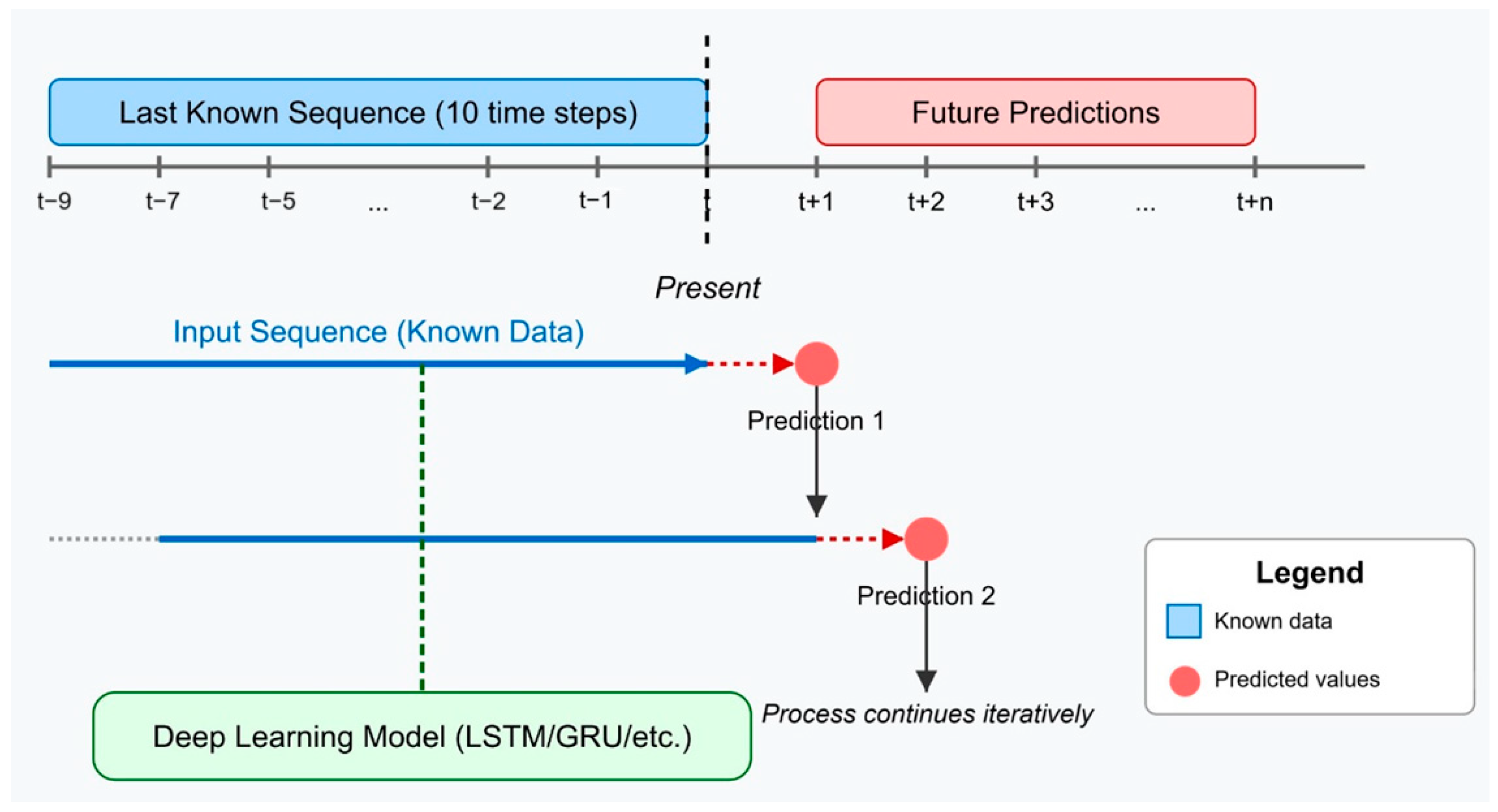
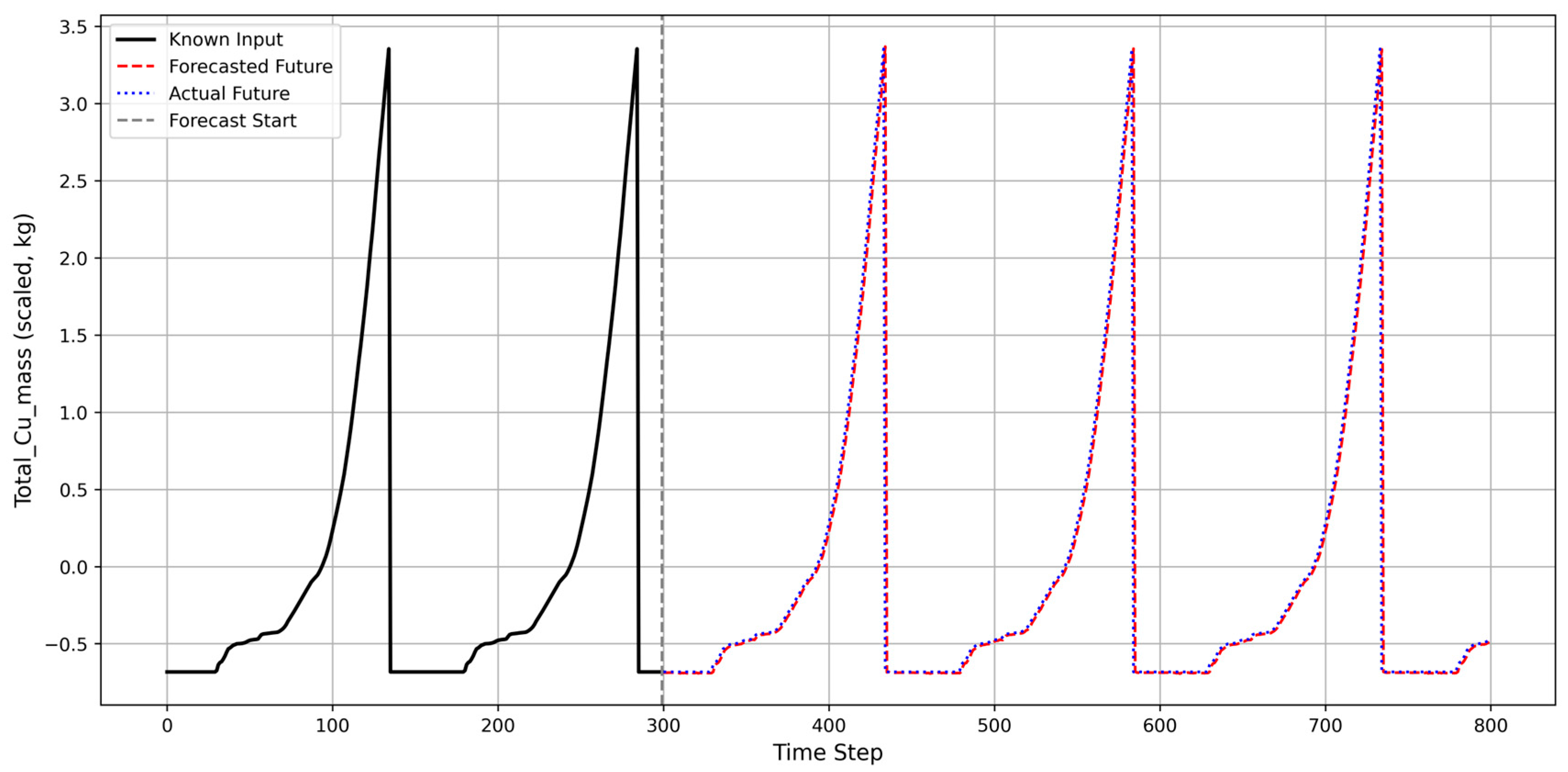
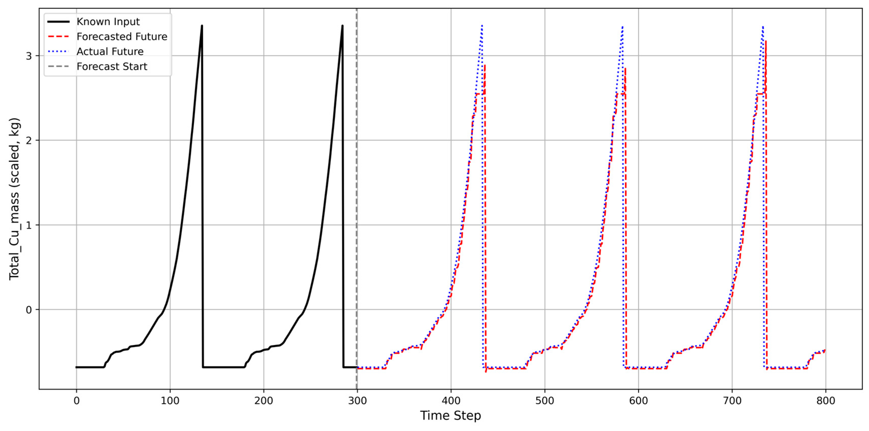
3.4.4. Forecasting Methodology

To assess the models’ ability to predict future values beyond the available data, an iterative forecasting procedure was implemented, as illustrated in Figure 2. Starting with the last known sequence from the dataset (appropriately scaled), each model generated a prediction for the next time step’s ‘Total_Cu_mass’. This predicted value (in its scaled form) was then used to update the input sequence for the subsequent prediction: the feature vector corresponding to the oldest time step in the sequence was discarded, and a new feature vector, identical to the last time step but with the ‘Total_Cu_mass’ feature replaced by the model’s prediction, was appended.
The process above was repeated iteratively for a specified number of future steps. The resulting sequence of predicted scaled values was then inverse-transformed to obtain forecasts in the original units of ‘Total_Cu_mass’.

3.5. Implementation Details

All data processing, model implementation, training, and evaluation were implemented using the scikit-learn library (version 1.6.1). Custom neural network architectures, including model classes and optimization routines, were developed using PyTorch (version 2.6.0+cu124). Some visualizations were generated with Matplotlib (version 3.10.1) and draw.io (version 23.0.2). The computational environment was based on Python version 3.10.11.

4. Results and Discussion

This section presents the findings from training and evaluating the different deep learning architectures on the augmented time-series data for ‘Total_Cu_mass’ forecasting. We analyze model convergence, compare quantitative performance metrics, assess qualitative forecasting behavior, and discuss the implications and limitations of the approach.

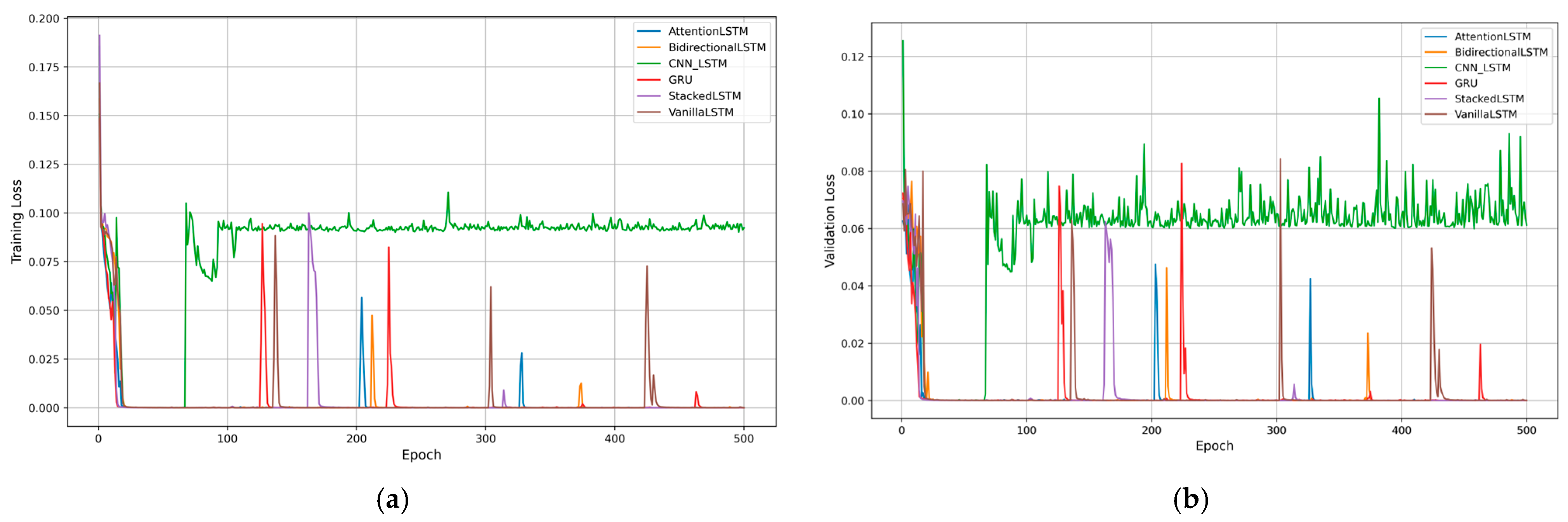
4.1. Training Dynamics

The learning progression of the models was monitored via training and validation loss curves across the 500 training epochs.
As depicted in Figure 3, the majority of the evaluated architectures (VanillaLSTM, StackedLSTM, BidirectionalLSTM, GRU, and AttentionLSTM) demonstrated efficient learning. They exhibited a sharp decrease in both training and validation loss during the initial epochs, quickly converging to very low loss values (near zero). The validation loss generally tracked the training loss closely for these models. This suggests that the models learned the patterns in the training data effectively without significant overfitting, aided by the early stopping criteria.
Conversely, the CNN-LSTM model displayed distinct training characteristics. Its convergence was notably slower, and both training and validation losses stabilized at substantially higher levels compared to the other models (Figure 3b shows validation loss fluctuating mostly between 0.05 and 0.10, while others are near 0). The validation loss curve for CNN-LSTM also showed higher volatility. This suggests that the specific CNN-LSTM configuration struggled to capture the temporal dependencies in this dataset as effectively as the purely recurrent or attention-augmented recurrent models.

4.2. Model Performance Evaluation

The predictive accuracy of the models was rigorously assessed using the held-out test set. Standard regression metrics were computed, comparing model predictions against the actual ‘Total_Cu_mass’ values.
Five of the six models achieved outstanding performance on the test data. VanillaLSTM, StackedLSTM, BidirectionalLSTM, GRU, and AttentionLSTM all yielded extremely low MAE and RMSE values (RMSE < 0.008) and R2 values exceeding 0.9999 (Table 2, Figure 4b). This indicates a very high degree of accuracy in predicting the next time step’s value within the structure of the augmented data.
Among the top performers, the BidirectionalLSTM (Test RMSE: 0.003) and AttentionLSTM (Test MAE: 0.002, Test RMSE: 0.004) models showed a slight edge by demonstrating the lowest error metrics overall (Table 2). The StackedLSTM and GRU models followed closely, also delivering notable accuracy.
The CNN-LSTM model clearly underperformed relative to its counterparts. Its test RMSE of 0.266 was significantly higher (Figure 4a), and its R2 score, while still high at 0.926, was substantially lower than the near-perfect scores of the others (Figure 4b). The high MAPE of 9.71% further underscores its reduced precision compared to the other architectures, which mostly achieved MAPE below 1.5%. The CNN-LSTM model’s lower performance likely stems from the mismatch between its architecture and the temporal dynamics of our copper extraction process. The CNN layer’s fixed kernel size and temporal smoothing effects may have disrupted the fine-grained sequential patterns crucial for this cyclical process. This architectural limitation prevented the model from capturing the subtle time dependencies that the pure recurrent architectures preserved successfully.
To gain further insight into the decision-making process of the Attention LSTM model, which demonstrated strong predictive performance (Table 2), we analyzed the characteristics of the time steps that the attention mechanism identified as most influential. This analysis was conducted on 1484 sequences from the test set.
First, we identified the time steps within each input sequence that received the top three highest attention weights. We then computed the average feature vector for all time steps that ranked as Top-1 attended, Top-2 attended, and Top-3 attended, respectively. Figure 5 illustrates these average feature profiles.
For the Top-1 attended steps (left panel), features such as ‘Pond Raf. Sol. Volume (m3)’, ‘Pond Prod. Sol. Volume (m3)’, and ‘EL Efficiency Sol (%)’ exhibit notable positive average scaled values, while ‘Cu_org_O (g/L)’ (copper in organic phase after loading) and ‘Cu_feed (g/L)’ show distinct negative average scaled values. This suggests that when the model places the highest importance on a time step, it might be focusing on periods characterized by, for instance, higher pond volumes and lower copper concentrations in the organic phase or feed (in scaled terms), potentially reflecting a particular stage or transition in the cyclical process.
The feature ‘Total Cu Mass (kg)’ (representing the target variable from previous steps within the input window) consistently shows a significant negative average scaled value in the Top-1 and Top-2 attended steps. This indicates the model’s strong reliance on the recent scaled trajectory of the target variable itself when identifying the most salient past information, a common characteristic in effective time-series forecasting models.
Comparing the top attended ranks, ‘Pond Raf. Sol. Volume (m3)’ consistently appears with a large positive scaled magnitude, highlighting its persistent importance. Conversely, ‘Ore Mass (tons)’ and ‘Initial Cu Mass (kg)’ generally show smaller, near-zero average scaled values at these critical attended steps, suggesting they might be less dynamically indicative for immediate next-step prediction compared to other process variables.
Second, to understand if the model consistently focuses on particular temporal positions within the 10-step input window, we analyzed the frequency with which each time step (index 0 to 9) appeared at each of the top-k attention ranks. Figure 6 shows this distribution.
For the Top-1 attended rank (blue line), there is a prominent peak at time step index 1 (the second most recent observation in the 10-step window before the prediction point). This suggests that the model very frequently finds the information from two days prior to be the most critical for predicting the next day’s copper mass.
The attention for Top-1 then drops significantly for more distant past steps, although there is a smaller secondary peak around indexes 4–5. For Top-2 and Top-3 attended ranks (orange and green lines), the attention is more distributed across the sequence, but still shows some preference. For example, time step index 2 (three days prior) often appears as the Top-2 attended step, and indexes 4–5 or 7 are also frequently selected for Top-2 or Top-3 ranks.
Notably, the very first step in the sequence (index 0, most distant in the 10-day window) and the most recent step (index 9, immediately preceding the prediction) are less frequently assigned the highest (Top-1) attention, though they do contribute at lower attention ranks.
Together, these analyses provide valuable insights into the Attention LSTM’s behavior. The model learns which feature characteristics are important (Figure 5) and also dynamically identifies specific time steps within the recent history that are most salient for prediction (Figure 6), with a strong tendency to prioritize information from one to two days prior for its highest attention. This offers a degree of explainability to the Attention LSTM’s strong performance and its decision-making basis.

4.3. Forecasting Capability

Beyond single-step prediction accuracy, the models’ ability to generate multi-step-ahead forecasts iteratively was examined. Using a 300-step history from the test set, forecasts of the best performing model (BidirectionalLSTM) and the worst performing model (CNN-LSTM) were generated for the subsequent 500 time steps and compared against the actual values.
The forecast continuation plots reveal a critical capability: all models, including the less accurate CNN-LSTM, were able to successfully learn and reproduce the pronounced cyclical pattern present in the ‘Total_Cu_mass’ data over an extended forecast horizon. The sharp peaks and troughs characteristic of the original 150-day cycle were replicated across multiple subsequent synthetic cycles in the forecast.
For the top-performing model (Figure 7), the forecasted trajectory (red dashed line) aligns remarkably well with the actual future data from the test set (blue dotted line). This shows that the model effectively captured the underlying dynamics governing the process variability as represented in the augmented dataset. The ability to extrapolate this pattern accurately for hundreds of steps ahead, based on training data derived from a single initial cycle via augmentation, is a significant result. While the CNN-LSTM (Figure 8) also captures the overall pattern, visual inspection suggests potential deviations in peak timing or amplitude, consistent with its higher quantitative error metrics.
The close alignment between the forecasts of the top and the actual test data trajectory speaks to their potential utility. This capability resonates with the need for advanced modeling to handle process uncertainties [37] and support complex decision-making in hydrometallurgical plants [29].
To provide a more rigorous quantitative assessment of this multi-step forecasting capability, the RMSE and MAPE were calculated at various forecast horizons (h = 10, 50, 100, and 500 steps) for the Bidirectional LSTM, Attention LSTM, and CNN-LSTM models. These metrics were derived from the iterative forecasting process using scaled data, consistent with the single-step evaluations. The results are summarized in Table 3.
The quantitative results in Table 3 corroborate the qualitative observations from Figure 5 and Figure 6. Both Bidirectional LSTM and Attention LSTM demonstrate strong performance in multi-step forecasting and maintain a relatively stable and low RMSE and MAPE values even up to 500 steps ahead. For instance, at h = 500, the Attention LSTM achieved an RMSE of 0.0511 and a MAPE of 6.76%, indicating a robust capability to extrapolate the learned cyclical patterns with considerable accuracy over extended horizons. The Bidirectional LSTM shows comparable stability, with a MAPE of 7.07% at h = 500. These values, while higher than single-step prediction errors, as expected due to error accumulation in iterative forecasting, are still indicative of good predictive coherence.
In contrast, the CNN-LSTM model exhibits markedly higher errors across all forecast horizons. Its MAPE increases to 12.35% at h = 500, roughly double that of the Attention LSTM. This larger error accumulation quantitatively confirms that the CNN-LSTM architecture, while able to reproduce the general cyclical shape, is less effective at preserving the precise temporal dependencies required for accurate long-range iterative forecasting within this augmented dataset. These findings further highlight the suitability of architectures like Bidirectional LSTM and Attention LSTM for applications requiring extended multi-step predictions of the cyclical copper production process, based on the patterns learned from the augmented data.

4.4. Discussion

The high predictive accuracy achieved, particularly by BiLSTM and AttentionLSTM, signifies the considerable potential of deep learning models for enhancing the predictability and potentially the control of complex hydrometallurgical copper extraction processes. Accurate forecasting of key variables like ‘Total_Cu_mass’ can contribute directly to the goals of sustainable metallurgy outlined previously: optimizing resource utilization, minimizing environmentally detrimental reagent overuse [8,9,10], reducing waste streams [1,2,3,4,16], and improving overall process efficiency [11].
A significant methodological contribution of this study lies in demonstrating the utility of data augmentation from limited initial data. Obtaining extensive, high-frequency data from industrial processes can be challenging and costly. Our results show that even starting with a single 150-day cycle, augmenting these data by introducing realistic noise allowed us to train sophisticated models that captured the core dynamics of the process, particularly its cyclical nature. This approach offers a pragmatic pathway for developing data-driven models in data-scarce industrial environments, a common challenge when implementing digital transformation strategies [34].
However, the reliance on this specific augmentation strategy constitutes the primary limitation. The models’ performance was validated on test data generated through the same augmentation mechanism applied to segments of the original cycle. While successful in replicating the known patterns, the generalization of these models to truly unseen, independent operational data remains unconfirmed. Thus, the high accuracy metrics primarily demonstrate strong self-consistency and the models’ capacity to learn the intricacies of the augmented data, rather than confirmed generalization to unseen, independent real-world operational periods. Real-world processes are subject to drifts, novel events, changes in feedstock quality [6], variations in reagent effectiveness [15,27], or different noise characteristics not fully captured by the simple Gaussian noise added to the original 150-day template. Therefore, the models’ robustness to conditions outside the scope of the initial observation period needs rigorous testing.
To bridge the gap towards reliable industrial deployment and fully realize the potential for sustainability improvements, future work will prioritize testing the leading models (BiLSTM, AttentionLSTM) against new data collected from subsequent, independent operational periods of the copper extraction plant without retraining the models. This will provide a true measure of their generalization capabilities. Moreover, there should be exploration of more sophisticated methods like Generative Adversarial Networks (GANs) or physics-informed modeling to generate synthetic data that better capture the complexities and potential anomalies of the real process.
To provide insights to domain experts, applying model interpretation techniques (e.g., SHAP [42]) to understand why the models make certain predictions, potentially linking feature importance back to specific hydrometallurgical principles or operational events, is essential [22,26]. It will also be beneficial to investigate how these predictive models could be integrated into decision support [29] or advanced process control frameworks to actively optimize operations towards sustainability goals.
This work successfully demonstrates that deep learning models, particularly BiLSTM and AttentionLSTM, trained on augmented data derived from limited initial observations, can achieve high accuracy in forecasting a key variable in a cyclical copper extraction process. This capability is particularly valuable for long-term production planning, resource allocation, and sustainability optimization in industrial operations. Nonetheless, validation on independent real-world data is a critical prerequisite for practical implementation.

5. Conclusions

This study successfully demonstrates the applicability and efficacy of deep learning approaches for predicting copper production metrics in hydrometallurgical processes, addressing the significant challenge of limited industrial data through strategic data augmentation. Our comprehensive evaluation of six recurrent neural network architectures revealed several important findings with implications for both the machine learning and hydrometallurgical domains.
First, our results establish that five of the six tested architectures—particularly Bidirectional LSTM and Attention LSTM—can achieve exceptional predictive accuracy (RMSE < 0.004, R2 > 0.999) for copper mass forecasting when trained on properly augmented time-series data. The Bidirectional LSTM’s superior performance underscores the value of processing sequential information in both forward and backward directions for capturing complex temporal dependencies in hydrometallurgical processes, while the Attention LSTM’s comparable accuracy highlights the importance of dynamically weighting relevant time steps when making predictions.
Second, we validated that even with data from a single 150-day operational cycle, appropriate augmentation can generate sufficient training data for developing highly accurate predictive models. This finding offers a practical solution to the persistent challenge of data scarcity in industrial settings, where extensive historical datasets are often unavailable due to monitoring limitations or proprietary constraints.
Third, our multi-step forecasting experiments demonstrated that the developed models can maintain prediction coherence over extended horizons (up to 500 time steps), successfully reproducing the cyclical patterns characteristic of copper extraction processes. This capability is particularly valuable for long-term production planning, resource allocation, and sustainability optimization in industrial operations.
However, we acknowledge important limitations that must be addressed in future work. The models’ performance was validated on test data generated through the same augmentation mechanism, which may not fully represent the complexity and variability of truly independent operational periods. Real-world process variations, including unexpected events, feedstock quality changes, and equipment aging effects, could introduce challenges not captured in our current approach.
Future research should focus on three key directions: (1) validating these models against independently collected operational data from subsequent production cycles; (2) exploring more sophisticated data augmentation techniques such as Generative Adversarial Networks or physics-informed modeling that could better represent process anomalies and edge cases; and (3) implementing model interpretation frameworks to provide actionable insights to process engineers and operators.
In conclusion, this work establishes a promising foundation for implementing AI-driven predictive systems in hydrometallurgical copper production. By enhancing process predictability and control, such systems can contribute significantly to the industry’s sustainability goals—reducing waste generation, optimizing reagent use, lowering energy consumption, and minimizing environmental impacts. The methodological approach demonstrated here, including the data augmentation strategy from limited cyclical data and the comparative evaluation of deep learning architectures, holds promise for adaptability to other metal extraction processes that exhibit similar time-series characteristics and face comparable data scarcity and sustainability challenges. While the specific input features and model parameters would need recalibration based on the unique chemistry and operational dynamics of other metal systems (e.g., gold, nickel, zinc), the core framework for developing predictive models could be transferable.

Author Contributions

Conceptualization, B.K.; methodology, A.K.; software, N.A. and B.A.; validation, S.A. and D.M.; formal analysis, B.K.; investigation, S.A.; resources, A.K.; data curation, A.K. and D.M.; writing—original draft preparation, N.A.; writing—review and editing, B.A. and A.K.; visualization, N.A.; supervision, B.A.; project administration, B.K.; funding acquisition, B.K. All authors have read and agreed to the published version of the manuscript.

Funding

This research was funded by the Committee of Science of the Ministry of Science and Higher Education of the Republic of Kazakhstan (Grant No. BR21882140).

Data Availability Statement

The data are not publicly available due to confidentiality agreements with the Institute of Metallurgy and Ore Beneficiation.

Acknowledgments

We would like to thank the Institute of Metallurgy and Ore Beneficiation for providing access to critical data and their invaluable support in facilitating this research.

Conflicts of Interest

The authors declare no conflicts of interest.

Appendix A

Figure A1. Pairwise relationships between features in the expanded synthetic dataset.
Minerals 15 00702 g0a1

References

  1. Kenzhaliyev, B.; Imankulov, T.; Mukhanbet, A.; Kvyatkovskiy, S.; Dyussebekova, M.; Tasmurzayev, N. Intelligent System for Reducing Waste and Enhancing Efficiency in Copper Production Using Machine Learning. Metals 2025, 15, 186. [Google Scholar] [CrossRef]
  2. Vives Pons, J.; Comerma, A.; Escobet, T.; Dorado, A.D.; Tarrés-Puertas, M.I. Optimizing Bioleaching for Printed Circuit Board Copper Recovery: An AI-Driven RGB-Based Approach. Appl. Sci. 2024, 15, 129. [Google Scholar] [CrossRef]
  3. Koizhanova, A.K.; Kenzhaliyev, B.K.; Magomedov, D.R.; Erdenova, M.B.; Bakrayeva, A.N.; Abdyldaev, N.N. Hydrometallurgical Studies on the Leaching of Copper from Man-Made Mineral Formations. Complex Use Miner. Resour. 2024, 330, 32–42. [Google Scholar] [CrossRef]
  4. Fan, X.; Wu, N.; Sun, L.; Jiang, Y.; He, S.; Huang, M.; Yang, K.; Cao, Y. New Separation Technology for Lead and Mercury from Acid Sludge of Copper Smelting Using a Total Hydrometallurgical Process. Min. Metall. Explor. 2024, 41, 1597–1604. [Google Scholar] [CrossRef]
  5. Dias, J.; De Holanda, J.N.F.; Pinho, S.C.; De Miranda Júnior, G.M.; Da Silva, A.G.P. Systematic LCA-AHP Approach to Compare Hydrometallurgical Routes for Copper Recovery from Printed Circuit Boards: Environmental Analysis. Sustainability 2024, 16, 8002. [Google Scholar] [CrossRef]
  6. Cheje Machaca, D.M.; Botelho, A.B.; De Carvalho, T.C.; Tenório, J.A.S.; Espinosa, D.C.R. Hydrometallurgical Processing of Chalcopyrite: A Review of Leaching Techniques. Int. J. Miner. Metall. Mater. 2024, 31, 2537–2555. [Google Scholar] [CrossRef]
  7. Koizhanova, A.; Kenzhaliyev, B.; Magomedov, D.; Kamalov, E.; Yerdenova, M.; Bakrayeva, A.; Abdyldayev, N. Study of Factors Affecting the Copper Ore Leaching Process. ChemEngineering 2023, 7, 54. [Google Scholar] [CrossRef]
  8. Martín, M.I.; García-Díaz, I.; López, F.A. Properties and Perspective of Using Deep Eutectic Solvents for Hydrometallurgy Metal Recovery. Miner. Eng. 2023, 203, 108306. [Google Scholar] [CrossRef]
  9. Gómez, M.; Grimes, S.; Fowler, G. Novel Hydrometallurgical Process for the Recovery of Copper from End-of-Life Mobile Phone Printed Circuit Boards Using Ionic Liquids. J. Clean. Prod. 2023, 420, 138379. [Google Scholar] [CrossRef]
  10. Godirilwe, L.L.; Haga, K.; Altansukh, B.; Jeon, S.; Danha, G.; Shibayama, A. Establishment of a Hydrometallurgical Scheme for the Recovery of Copper, Nickel, and Cobalt from Smelter Slag and Its Economic Evaluation. Sustainability 2023, 15, 10496. [Google Scholar] [CrossRef]
  11. Kenzhaliyev, B.; Amangeldy, B.; Mukhanbet, A.; Azatbekuly, N.; Koizhanova, A.; Magomedov, D. Development of Software for Hydrometallurgical Calculation of Metal Extraction. Complex Use Miner. Resour. 2024, 335, 78–88. [Google Scholar] [CrossRef]
  12. Şayan, E.; Çalışkan, B. The Use of Ultrasound in Hydrometallurgical Studies: A Review on the Comparison of Ultrasound-Assisted and Conventional Leaching. J. Sustain. Metall. 2024, 10, 1933–1958. [Google Scholar] [CrossRef]
  13. Ordaz-Oliver, M.; Jiménez-Muñoz, E.; Gutiérrez-Moreno, E.; Borja-Soto, C.E.; Ordaz, P.; Montiel-Hernández, J.F. Application of Artificial Neural Networks for Recovery of Cu from Electronic Waste by Dynamic Acid Leaching: A Sustainable Approach. Waste Biomass Valor 2024, 15, 7057–7076. [Google Scholar] [CrossRef]
  14. Oráč, D.; Klimko, J.; Klein, D.; Pirošková, J.; Liptai, P.; Vindt, T.; Miškufová, A. Hydrometallurgical Recycling of Copper Anode Furnace Dust for a Complete Recovery of Metal Values. Metals 2021, 12, 36. [Google Scholar] [CrossRef]
  15. Nizamoğlu, H.; Turan, M.D. Using of Leaching Reactant Obtained from Mill Scale in Hydrometallurgical Copper Extraction. Environ. Sci. Pollut. Res. 2021, 28, 54811–54825. [Google Scholar] [CrossRef]
  16. Binnemans, K.; Jones, P.T. The Twelve Principles of Circular Hydrometallurgy. J. Sustain. Metall. 2023, 9, 1–25. [Google Scholar] [CrossRef]
  17. Astudillo, Á.; Garcia, M.; Quezada, V.; Valásquez, L. The Use of Seawater in Copper Hydrometallurgical Processing in Chile: A Review. J. S. Afr. Inst. Min. Metall. 2023, 123, 357–364. [Google Scholar] [CrossRef]
  18. Amankwaa-Kyeremeh, B.; McCamley, C.; Zanin, M.; Greet, C.; Ehrig, K.; Asamoah, R.K. Prediction and Optimisation of Copper Recovery in the Rougher Flotation Circuit. Minerals 2023, 14, 36. [Google Scholar] [CrossRef]
  19. Amankwaa-Kyeremeh, B.; Ehrig, K.; Greet, C.; Asamoah, R. Pulp Chemistry Variables for Gaussian Process Prediction of Rougher Copper Recovery. Minerals 2023, 13, 731. [Google Scholar] [CrossRef]
  20. Zou, G.; Zhou, J.; Li, K.; Zhao, H. An HGA-LSTM-Based Intelligent Model for Ore Pulp Density in the Hydrometallurgical Process. Materials 2022, 15, 7586. [Google Scholar] [CrossRef]
  21. Murali, A.; Plummer, M.J.; Shine, A.E.; Free, M.L.; Sarswat, P.K. Optimized Bioengineered Copper Recovery from Electronic Wastes to Increase Recycling and Reduce Environmental Impact. J. Hazard. Mater. Adv. 2022, 5, 100031. [Google Scholar] [CrossRef]
  22. Ji, G.; Liao, Y.; Wu, Y.; Xi, J.; Liu, Q. A Review on the Research of Hydrometallurgical Leaching of Low-Grade Complex Chalcopyrite. J. Sustain. Metall. 2022, 8, 964–977. [Google Scholar] [CrossRef]
  23. Mohanty, U.; Rintala, L.; Halli, P.; Taskinen, P.; Lundström, M. Hydrometallurgical Approach for Leaching of Metals from Copper Rich Side Stream Originating from Base Metal Production. Metals 2018, 8, 40. [Google Scholar] [CrossRef]
  24. Panda, S.; Mishra, G.; Sarangi, C.K.; Sanjay, K.; Subbaiah, T.; Das, S.K.; Sarangi, K.; Ghosh, M.K.; Pradhan, N.; Mishra, B.K. Reactor and Column Leaching Studies for Extraction of Copper from Two Low Grade Resources: A Comparative Study. Hydrometallurgy 2016, 165, 111–117. [Google Scholar] [CrossRef]
  25. Xiao, Y.; Yang, Y.; Van Den Berg, J.; Sietsma, J.; Agterhuis, H.; Visser, G.; Bol, D. Hydrometallurgical Recovery of Copper from Complex Mixtures of End-of-Life Shredded ICT Products. Hydrometallurgy 2013, 140, 128–134. [Google Scholar] [CrossRef]
  26. Bergh, L.G.; Jämsä-Jounela, S.-L.; Hodouin, D. State of the Art in Copper Hydrometallurgic Processes Control. Control Eng. Pract. 2001, 9, 1007–1012. [Google Scholar] [CrossRef]
  27. Ashiq, A.; Kulkarni, J.; Vithanage, M. Hydrometallurgical Recovery of Metals From E-Waste. In Electronic Waste Management and Treatment Technology; Elsevier: Amsterdam, The Netherlands, 2019; pp. 225–246. ISBN 978-0-12-816190-6. [Google Scholar]
  28. Saldaña, M.; Neira, P.; Gallegos, S.; Salinas-Rodríguez, E.; Pérez-Rey, I.; Toro, N. Mineral Leaching Modeling Through Machine Learning Algorithms—A Review. Front. Earth Sci. 2022, 10, 816751. [Google Scholar] [CrossRef]
  29. Saldaña, M.; Neira, P.; Flores, V.; Robles, P.; Moraga, C. A Decision Support System for Changes in Operation Modes of the Copper Heap Leaching Process. Metals 2021, 11, 1025. [Google Scholar] [CrossRef]
  30. Flores, V.; Leiva, C. A Comparative Study on Supervised Machine Learning Algorithms for Copper Recovery Quality Prediction in a Leaching Process. Sensors 2021, 21, 2119. [Google Scholar] [CrossRef]
  31. Correa, P.P.; Cipriano, A.; Nuñez, F.; Salas, J.C.; Lobel, H. Forecasting Copper Electrorefining Cathode Rejection by Means of Recurrent Neural Networks With Attention Mechanism. IEEE Access 2021, 9, 79080–79088. [Google Scholar] [CrossRef]
  32. Caplan, M.; Trouba, J.; Anderson, C.; Wang, S. Hydrometallurgical Leaching of Copper Flash Furnace Electrostatic Precipitator Dust for the Separation of Copper from Bismuth and Arsenic. Metals 2021, 11, 371. [Google Scholar] [CrossRef]
  33. Brest, K.K.; Monga, K.J.J.; Henock, M.M. Implementation of Artificial Neural Network into the Copper and Cobalt Leaching Process. In Proceedings of the 2021 Southern African Universities Power Engineering Conference/Robotics and Mechatronics/Pattern Recognition Association of South Africa (SAUPEC/RobMech/PRASA), Potchefstroom, South Africa, 27–29 January 2021; pp. 1–5. [Google Scholar]
  34. Aleksandrova, T.N.; Orlova, A.V.; Taranov, V.A. Current Status of Copper-Ore Processing: A Review. Russ. J. Non-Ferrous Met. 2021, 62, 375–381. [Google Scholar] [CrossRef]
  35. Jia, L.; Huang, J.; Ma, Z.; Liu, X.; Chen, X.; Li, J.; He, L.; Zhao, Z. Research and Development Trends of Hydrometallurgy: An Overview Based on Hydrometallurgy Literature from 1975 to 2019. Trans. Nonferrous Met. Soc. China 2020, 30, 3147–3160. [Google Scholar] [CrossRef]
  36. Flores, V.; Keith, B.; Leiva, C. Using Artificial Intelligence Techniques to Improve the Prediction of Copper Recovery by Leaching. J. Sens. 2020, 2020, 1–12. [Google Scholar] [CrossRef]
  37. Saldaña, M.; González, J.; Jeldres, R.I.; Villegas, Á.; Castillo, J.; Quezada, G.; Toro, N. A Stochastic Model Approach for Copper Heap Leaching through Bayesian Networks. Metals 2019, 9, 1198. [Google Scholar] [CrossRef]
  38. Dildabek, A.; Abdiakhmetova, Z. Using Synthetic Data to Improve Data Processing Algorithms in Business Intelligence. J. Probl. Comput. Sci. Inf. Technol. 2024, 2, 44–49. [Google Scholar] [CrossRef]
  39. Daribayev, B.; Azatbekuly, N.; Mukhanbet, A. Optimization of Neural Networks for Predicting Oil Recovery Factor Using Quantization Techniques. J. Probl. Comput. Sci. Inf. Technol. 2024, 2, 25–33. [Google Scholar] [CrossRef]
  40. Amangeldy, B.; Tasmurzayev, N.; Shinassylov, S.; Mukhanbet, A.; Nurakhov, Y. Integrating Machine Learning with Intelligent Control Systems for Flow Rate Forecasting in Oil Well Operations. Automation 2024, 5, 343–359. [Google Scholar] [CrossRef]
  41. Glavackij, A.; David, D.P.; Mermoud, A.; Romanou, A.; Aberer, K. Beyond S-Curves: Recurrent Neural Networks for Technology Forecasting. arXiv 2022, arXiv:2211.15334. [Google Scholar] [CrossRef]
  42. Lundberg, S.; Lee, S.-I. A Unified Approach to Interpreting Model Predictions. arXiv 2017, arXiv:arXiv.1705.07874. [Google Scholar] [CrossRef]
Figure 1. Overview of the methodology employed in this study.
Minerals 15 00702 g001
Figure 2. Illustration of the iterative forecasting methodology used for multi-step-ahead predictions.
Minerals 15 00702 g002
Figure 3. Loss curves for all models: (a) training step; (b) validation step.
Minerals 15 00702 g003
Figure 4. Evaluation values for the different models and dataset splits. (a) RMSE; (b) R 2 .
Minerals 15 00702 g004
Figure 5. Average feature profiles for the Top-1, Top-2, and Top-3 most attended time steps by the Attention LSTM model across 1484 test sequences. Features (with units) are sorted by the absolute average scaled value of the Top-1 attended step. Values represent the average scaled feature magnitudes at these critical time steps.
Minerals 15 00702 g005
Figure 6. Frequency of each time step (index 0–9 within the 10-step input sequence) appearing at Top-1, Top-2, and Top-3 attention ranks across 1484 test sequences.
Minerals 15 00702 g006
Figure 7. BidirectionalLSTM forecasting.
Minerals 15 00702 g007
Figure 8. CNN-LSTM forecasting.
Minerals 15 00702 g008
Table 1. Copper extraction process dataset structure.
Variable NamePhysical Measurement (Units)Description
Cu_feedCopper concentration (g/L)Concentration of copper in the feed solution entering the extraction process
Cu_rafCopper concentration (g/L)Concentration of copper in the raffinate solution (the aqueous phase after extraction)
Extraction_flowFlow rate (m3/day)Volume flow rate of solution during the extraction stage
Cu_extr_effEfficiency (%)Percentage of copper successfully extracted from feed solution
Pond_prod_sol_volVolume (m3)Total volume of productive solution stored in the leaching pond
Pond_raf_sol_volVolume (m3)Total volume of raffinate solution stored in the pond
Cu_org_BCopper concentration (g/L)Concentration of copper in the organic phase before loading (entering re-extraction)
Cu_org_OCopper concentration (g/L)Concentration of copper in the organic phase after loading (leaving extraction)
Org_flowFlow rate (m3/day)Volume flow rate of the organic extractant through the system
Cu_el_BCopper concentration (g/L)Concentration of copper in the electrolyte before electrolysis
El_flow_BFlow rate (m3/day)Volume flow rate of the electrolyte before electrolysis
Cu_el_eff_orgEfficiency (%)Percentage efficiency of copper transfer from organic phase to electrolyte
Cu_el_eff_solEfficiency (%)Percentage efficiency of copper electrodeposition from solution to cathodes
Cu_el_OCopper concentration (g/L)Concentration of copper in the electrolyte after electrolysis
El_flow_OFlow rate (m3/day)Volume flow rate of the electrolyte after electrolysis
Cu_cat_growthMass growth rate (kg/day)Rate of copper deposition on cathodes during electrolysis
Total_Cu_massMass (kg)Total cumulative mass of copper produced (target variable)
Ore_to_metal_extrRatio (kg ore/kg Cu)Mass ratio of ore processed to metal extracted
Total_extraction_effEfficiency (%)Overall percentage efficiency of the entire extraction process
Ore_massMass (tons)Total mass of ore processed in the extraction operation
Initial_Cu_massMass (kg)Initial mass of copper in the ore before processing begins
Org_volumeVolume (m3)Total volume of organic extractant in the system
Table 2. Test set evaluation metrics for all models.
ModelMAERMSER2MAPE
VanillaLSTM0.0040.00811.456
Figure0.0030.00610.682
BidirectionalLSTM0.0020.00310.928
GRU0.0040.00511.361
CNN_LSTM0.0570.2660.9269.706
AttentionLSTM0.0020.00410.731
Table 3. Multi-step iterative forecasting performance (RMSE@h/MAPE@h (%)).
Modelh = 10h = 50h = 100h = 500
Bidirectional LSTM0.0480/6.84%0.0509/7.09%0.0510/6.68%0.0515/7.07%
Attention LSTM0.0475/6.31%0.0507/6.57%0.0508/6.24%0.0511/6.76%
CNN-LSTM0.1238/11.67%0.1333/12.28%0.1334/11.84%0.1336/12.35%
Disclaimer/Publisher’s Note: The statements, opinions and data contained in all publications are solely those of the individual author(s) and contributor(s) and not of MDPI and/or the editor(s). MDPI and/or the editor(s) disclaim responsibility for any injury to people or property resulting from any ideas, methods, instructions or products referred to in the content.

