
Advancing Flotation Process Modeling: Bayesian vs. Sklearn Approaches for Gold Grade Prediction


Abstract
1. Introduction
Research Gap
2. Materials and Methods
2.1. Data Description
2.2. Size Distribution of Crushed Product
2.3. Data Preprocessing
2.4. Bayesian Ridge Regression Models: Scikit-Learn vs. Pymc
2.4.1. Scikit-Learn Bayesian Ridge Regression
2.4.2. PyMC Probabilistic Programming
- Y is the vector of observed responses (e.g., y2 in flotation).
- X is the design matrix of input features (e.g., crusher type, particle size, power, collector type).
- β~N (0, λ−1I): is the vector of regression coefficients, representing the influence of each feature on the response. β has a zero-mean multivariate normal prior with isotropic covariance.
- ε~N (0, α − 1) is the random error term, following a zero-mean Gaussian distribution accounting for noise and model uncertainty.
- I is the identity matrix, ensuring that priors are independent across coefficients.
- Assumptions: Normal priors for β; multivariate normal priors for coefficients.
- optimization: The key hyperparameters (λ, α) were optimized through cross-validation, balancing model complexity and predictive accuracy.
- Pros: Custom modelling, richer uncertainty quantification, and posterior inference via MCMC.
2.4.3. Comparison and Justification
2.5. Feature and Target Variables
2.6. Feature Transformation to Enhance Model Performance
2.7. Cross-Validation
3. Results and Discussion
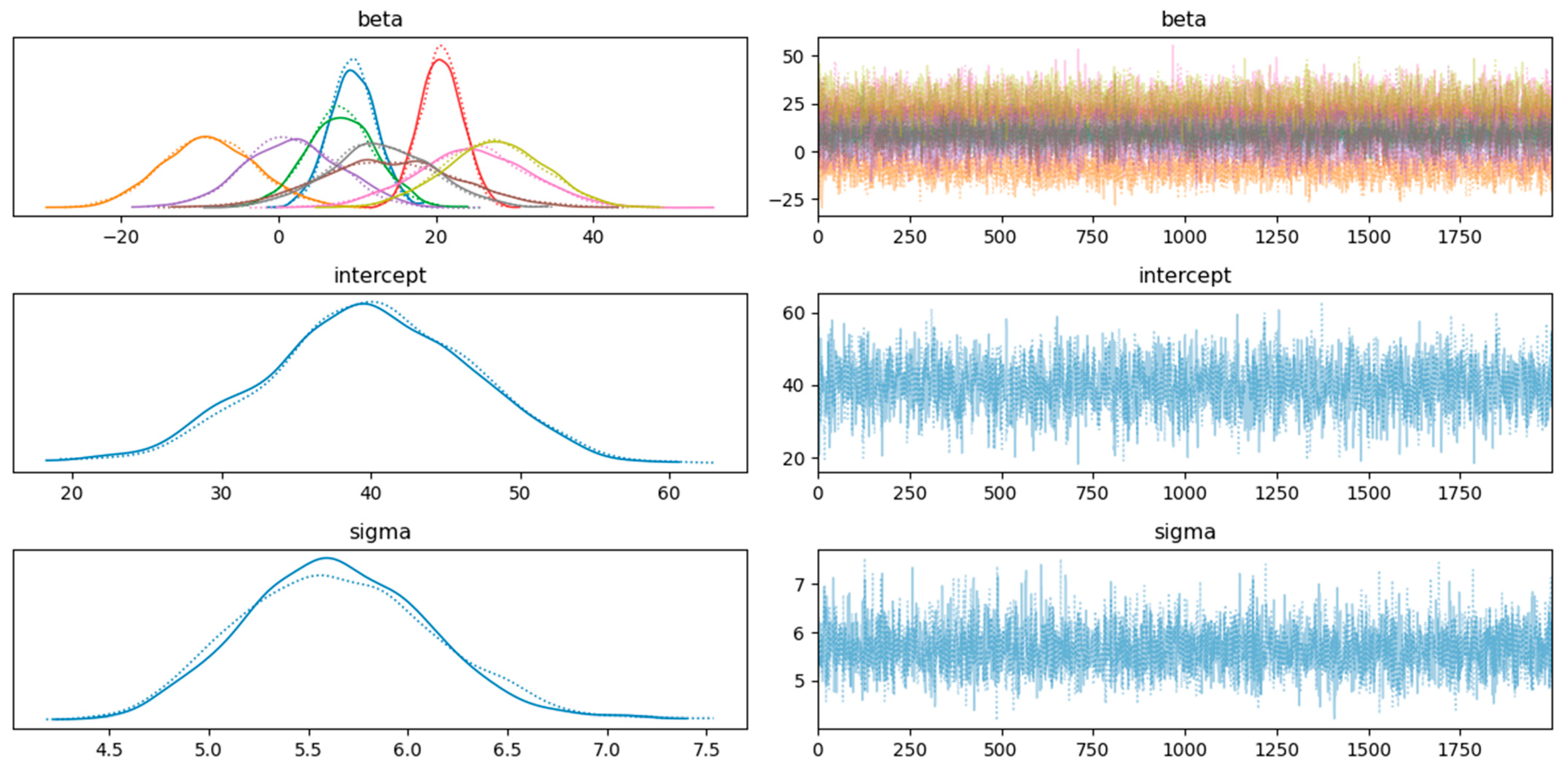
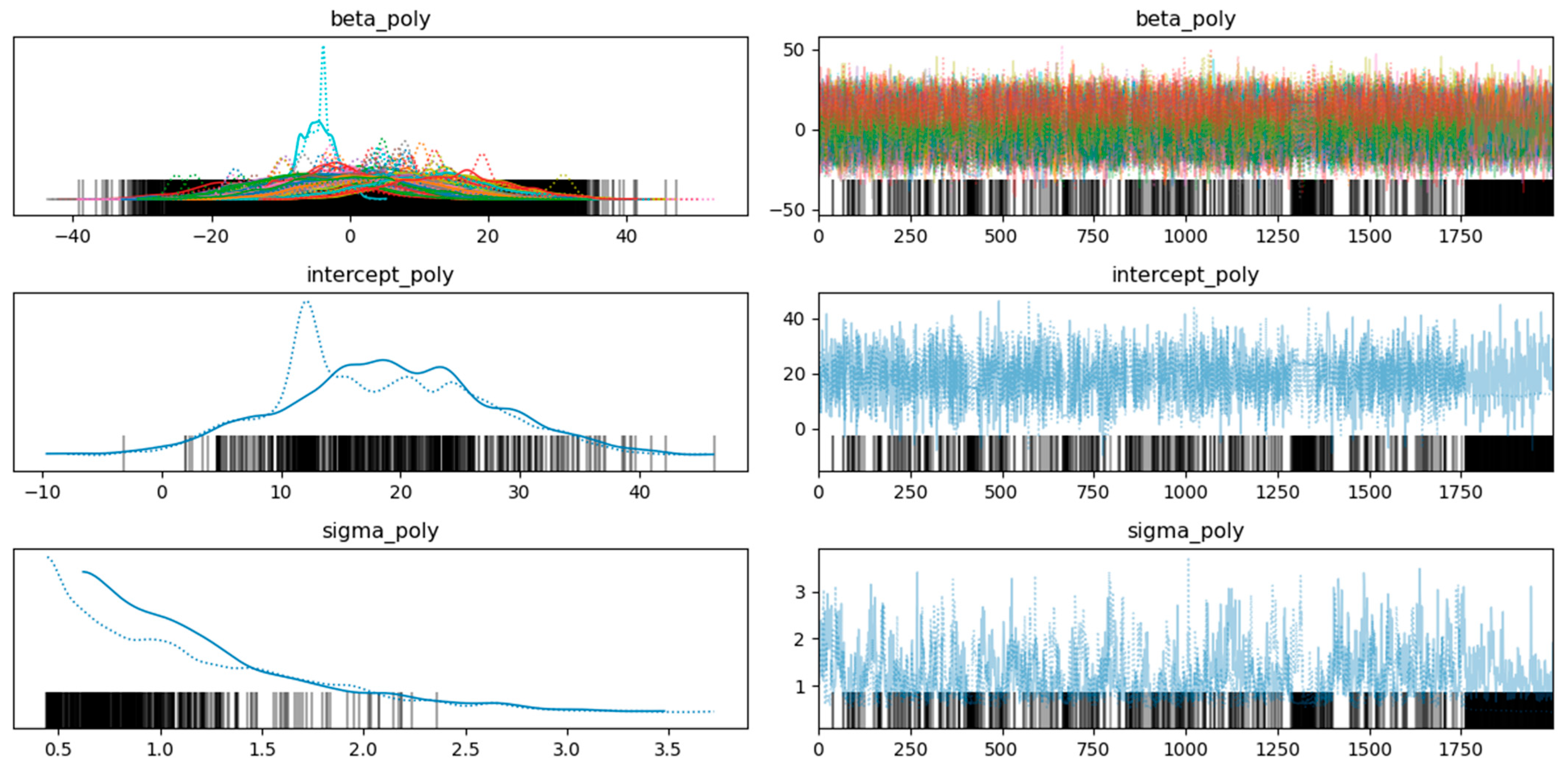
3.1. Cum_Grade Sampling Results
- Intercept distribution (second row, left):
- The bell-shaped curve labelled “alpha” represents the posterior distribution of the “Intercept”.
- The peak (around 40 for original and 20 for polynomial features) indicates the most likely value.
- The spread reflects the uncertainty or variability in the estimate.
- This curve combines prior information with the data likelihood to estimate the parameter.
- Intercept trace plot (second row, right):
- The trace plot for “Intercept” shows parameter values sampled during MCMC simulation.
- Each line represents a different chain or iteration, with fluctuations around the mean value (around 40 for original and 20 for polynomial) indicating convergence and stability.
- Well-mixed and converged chains suggest a reliable estimate for “alpha”.
- Beta1 distributions (top left):
- Multiple overlapping curves labelled “beta” represent the posterior distributions for different categories or groups.
- Variations in peak and spread indicate differences between these groups.
- Beta1 trace plot (top right):
- The trace plot for “beta1” shows sampled values during MCMC.
- Different colours represent different chains or iterations, with convergence and stability essential for reliable parameter estimates.
- Sigma1 distribution (bottom row, left):
- The bell-shaped curve labelled “sigma1” represents the posterior distribution of “sigma1”.
- The peak (around 5.6 for original and ~1 for polynomial) indicates the most likely value.
- The spread reflects uncertainty.
- Sigma1 trace plot (third row, right):
- The trace plot for “sigma1” shows sampled values during MCMC.
- Stability and convergence are crucial for reliable estimates.
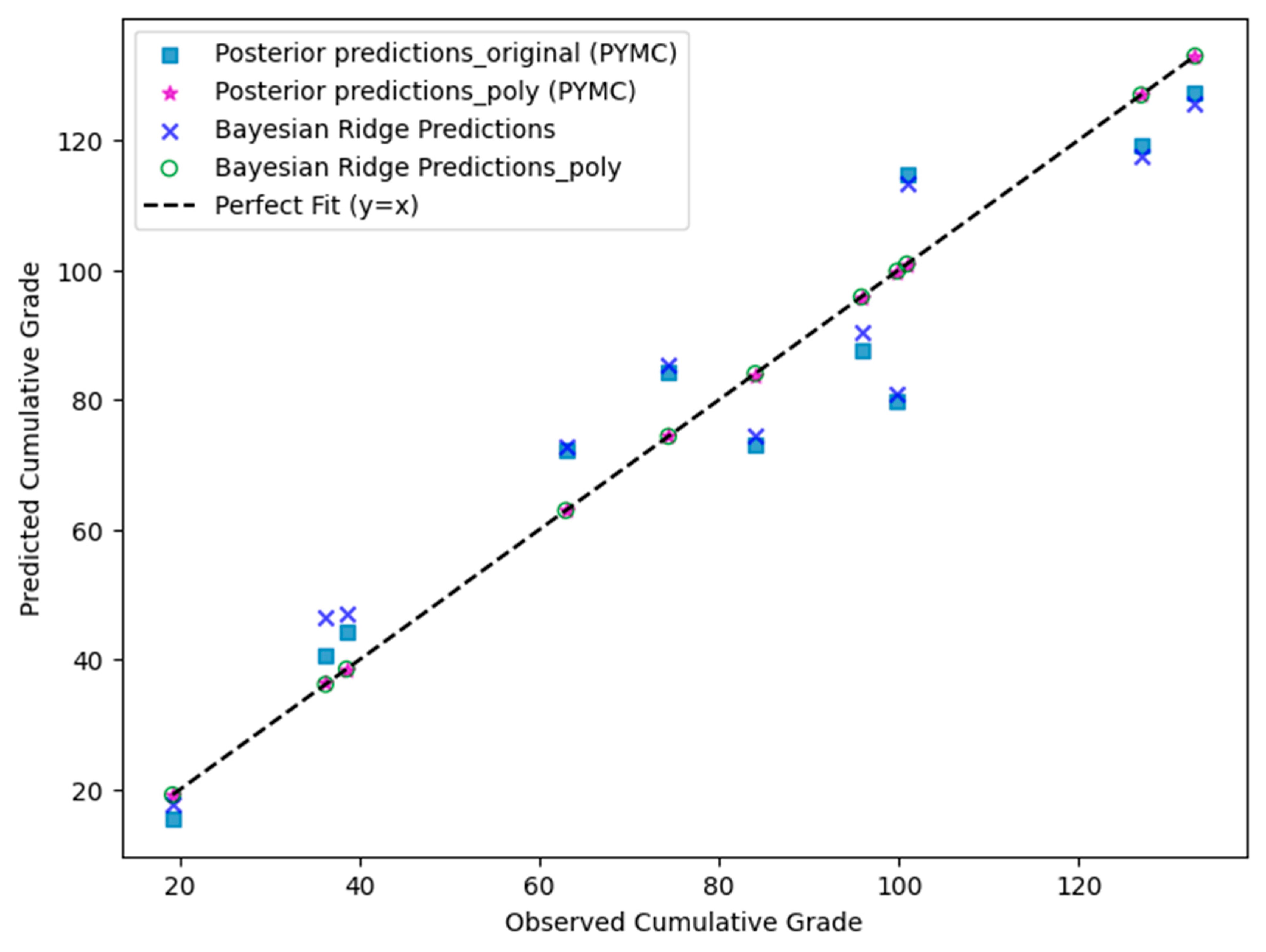
3.2. Model Performance (Table 6 (Original Features) and 7 (Polynomial Features))
3.3. Comparison of Models:
4. Scientific Significance of Bayesian Models
5. Conclusions
Funding
Data Availability Statement
Acknowledgments
Conflicts of Interest
Appendix A
Significant Model Factors or Hyperparameters of Bayesian Linear Ridge Regression
Appendix B
Appendix C
- Mean: Average estimated value of the coefficient.
- SD: Standard deviation, measuring variability of coefficient estimates.
- HDI 3%: Lower bound of the 94% probability interval for the true value.
- HDI 97%: Upper bound of the 94% probability interval for the true value.
- MCSE Mean: Accuracy of the mean estimate.
- MCSE SD: Accuracy of the standard deviation estimate.
- ESS Bulk: Effective sample size of the bulk of the distribution.
- ESS Tail: Effective sample size of the tails of the distribution.
- R-hat: Convergence diagnostic, with values near 1 indicating good convergence.
- Beta (β): Coefficients showing the relationship between predictors and the dependent variable.
- Sigma (σ): Standard deviation of residuals, indicating data variability around the regression line.
References
- Arbiter, N.; Harris, C. Flotation Kinetics. In Froth Flotation; AIME: Vancouver, BC, Canada, 1962; pp. 215–246. [Google Scholar]
- Kohmuench, J.; Thanasekaran, H.; Seaman, B. Advances in Coarse Particle Flotation-Copper and Gold. In Proceedings of the MetPlant 2013, Perth, Australia, 15–17 July 2013; The Australasian Institute of Mining and Metallurgy: Carlton, Australia, 2013; pp. 378–386. [Google Scholar]
- Estay, H.; Lois-Morales, P.; Montes-Atenas, G.; del Solar, J.R. On the Challenges of Applying Machine Learning in Mineral Processing and Extractive Metallurgy. Minerals 2023, 13, 788. [Google Scholar] [CrossRef]
- Jovanović, I.; Nakhaei, F.; Kržanović, D.; Conić, V.; Urošević, D. Comparison of Fuzzy and Neural Network Computing Techniques for Performance Prediction of an Industrial Copper Flotation Circuit. Minerals 2022, 12, 1493. [Google Scholar] [CrossRef]
- Nakhaei, F.; Rahimi, S.; Fathi, M. Prediction of Sulfur Removal from Iron Concentrate Using Column Flotation Froth Features: Comparison of k-Means Clustering, Regression, Backpropagation Neural Network, and Convolutional Neural Network. Minerals 2022, 12, 1434. [Google Scholar] [CrossRef]
- Yan, H.; Zhu, J.; Wang, F.; He, D.; Wang, Q. Bayesian Network-based Technical Index Estimation for Industrial Flotation Process under Incomplete Data. In Proceedings of the Chinese Control and Decision Conference (CCDC), Hefei, China, 22–24 August 2020. [Google Scholar]
- Kruschke, J.K. Doing Bayesian Data Analysis: A Tutorial with R, JAGS, and Stan; Academic Press: Cambridge, MA, USA, 2014. [Google Scholar]
- Gelman, A.; Carlin, J.B.; Stern, H.S.; Dunson, D.B.; Vehtari, A.; Rubin, D.B. Bayesian Data Analysis, 3rd ed.; CRC Press: Boca Raton, FL, USA, 2013. [Google Scholar]
- Yan, H.; Wang, F.; He, D.; Zhao, L.; Wang, Q. Bayesian Network-Based Modeling and Operational Adjustment of Plantwide Flotation Industrial Process. Ind. Eng. Chem. Res. 2020, 59, 2025–2035. [Google Scholar] [CrossRef]
- Yan, H.; Song, S.; Wang, F.; He, D.; Zhao, J. Operational adjustment modeling approach based on Bayesian network transfer learning for new flotation process under scarce data. J. Process Control 2023, 128, 103000. [Google Scholar] [CrossRef]
- Fu, H.; Wang, Z.; Nichani, E.; Lee, J.D. Learning Hierarchical Polynomials of Multiple Nonlinear Features with Three-Layer Networks. arXiv 2024, arXiv:2411.17201. [Google Scholar]
- PyMC. 2021. Available online: https://www.pymc.io/projects/docs/en/stable/learn.html (accessed on 1 January 2021).
- Thatipamula, S.; Devasahayam, S. Study of Coarse and Fine Gold Flotation on the Products from Vertical Shaft Impactor and High-Pressure Grinding Roll Crushers-submitted:MINE-D-23-01610. SSRN 4727563. Available online: https://dx.doi.org/10.2139/ssrn.4727563 (accessed on 14 January 2024).
- Albon, C. Machine Learning with Python Cookbook, 1st ed.; Bleiel, R.R.A.J., Ed.; O’Reilly Media: Sebastopol, CA, USA, 2018; p. 366. [Google Scholar]
- Pedregosa, F.; Varoquaux, G.; Gramfort, A.; Michel, V.; Thirion, B.; Grisel, O.; Blondel, M.; Prettenhofer, P.; Weiss, R.; Dubourg, V.; et al. sklearn.linear_model.BayesianRidge. J. Mach. Learn. Res. 2011, 12, 2825–2830. [Google Scholar]
- Salvatier, J.; Wiecki, T.V.; Fonnesbeck, C. Probabilistic programming in Python using PyMC3. PeerJ Comput. Sci. 2016, 2, e55. [Google Scholar] [CrossRef]
- Brownlee, J. Blending Ensemble Machine Learning with Python. 2021. Available online: https://machinelearningmastery.com/blending-ensemble-machine-learning-with-python/ (accessed on 11 May 2022).
- Devasahayam, S. Deep learning models in Python for predicting hydrogen production: A comparative study. Energy 2023, 280, 128088. [Google Scholar] [CrossRef]
- Devasahayam, S.; Albijanic, B. Predicting hydrogen production from co-gasification of biomass and plastics using tree based machine learning algorithms. Renew. Energy 2024, 222, 119883. [Google Scholar] [CrossRef]

| Phase | Weight % |
|---|---|
| Quartz | 50 |
| Muscovite | 18 |
| Fe-Dolomite/ankerite | 11.5 |
| Chlorite | 7.9 |
| Siderite | 4.2 |
| Kaolinite | 3.4 |
| Albite | 3.3 |
| Rutile | 0.8 |
| Pyrite | 0.9 |
| Crusher | Size, µm | Power (Crusher), kW | Time for Producing Required Size, s | Head Grade, g/t | Cum_Recovery, % | Cumulative Gold Grade g/t | Collector |
|---|---|---|---|---|---|---|---|
| HS-HPGR (600 µm) | 600 | 7.97 | 30 | 2.32 | 80.67 | 74.32 | PAX |
| LS-HPGR (600 µm) | 600 | 13.55 | 41.5 | 1.09 | 85.45 | 38.51 | PAX |
| VSI (600 µm) | 600 | 5.42 | 28 | 2.70 | 86.15 | 132.92 | PAX |
| HS-HPGR (425 µm) | 425 | 7.80 | 33 | 2.34 | 87.09 | 83.99 | PAX |
| LS-HPGR (425 µm) | 425 | 13.83 | 95 | 2.12 | 83.80 | 99.77 | PAX |
| VSI (425 µm) | 425 | 5.52 | 40 | 2.76 | 90.78 | 126.91 | PAX |
| HS-HPGR (300 µm) | 300 | 7.29 | 36 | 0.84 | 79.98 | 19.15 | PAX |
| LS-HPGR (300 µm) | 300 | 14.48 | 122 | 2.00 | 93.93 | 62.90 | PAX |
| VSI (300 µm) | 300 | 5.78 | 50 | 2.85 | 93.69 | 100.85 | PAX |
| VSI (300 µm) | 300 | 5.78 | 50 | 2.46 | 89.26 | 95.8 | DSP |
| HS-HPGR (300 µm) | 300 | 7.29 | 36 | 2.02 | 88.72 | 36.17 | DSP |
| Statistic | Size | Power | Time | Head_Grade | Cum_Recovery | Cum_Grade |
|---|---|---|---|---|---|---|
| count | 11.00 | 11.00 | 11.00 | 11.00 | 11.00 | 11.00 |
| mean | 415.91 | 8.61 | 52.82 | 2.14 | 87.23 | 79.21 |
| std | 130.03 | 3.55 | 29.42 | 0.65 | 4.66 | 37.09 |
| min | 300.00 | 5.42 | 30.00 | 0.84 | 79.98 | 19.15 |
| 25% | 300.00 | 5.78 | 34.50 | 2.01 | 84.63 | 50.71 |
| 50% | 425.00 | 7.29 | 41.50 | 2.32 | 87.09 | 83.99 |
| 75% | 512.50 | 10.76 | 55.00 | 2.58 | 90.02 | 100.31 |
| max | 600.00 | 14.48 | 122.00 | 2.85 | 93.93 | 132.92 |
| Category | Crusher | Collector |
|---|---|---|
| DSP | NaN | 2.0 |
| HPGRHS | 4.0 | NaN |
| HPLS | 3.0 | NaN |
| PAX | NaN | 9.0 |
| VSI | 4.0 | NaN |
| Size, µm | Power (Crusher), kW | Time for Producing Required Size, s | Head Grade, g/t | Crusher HS_HPGR | Crusher LS_HPGR | Crusher VSI | Collector, DSP | Collector, PAX |
|---|---|---|---|---|---|---|---|---|
| 600 | 7.97 | 30 | 2.32 | 1 | 0 | 0 | 0 | 1 |
| 600 | 13.55 | 41.5 | 1.09 | 0 | 1 | 0 | 0 | 1 |
| 600 | 5.42 | 28 | 2.70 | 0 | 0 | 1 | 0 | 1 |
| 425 | 7.80 | 33 | 2.34 | 1 | 0 | 0 | 0 | 1 |
| 425 | 13.83 | 95 | 2.12 | 0 | 1 | 0 | 0 | 1 |
| 425 | 5.52 | 40 | 2.76 | 0 | 0 | 1 | 0 | 1 |
| 300 | 7.29 | 36 | 0.84 | 1 | 0 | 0 | 0 | 1 |
| 300 | 14.48 | 122 | 2.00 | 0 | 1 | 0 | 0 | 1 |
| 300 | 5.78 | 50 | 2.85 | 0 | 0 | 1 | 0 | 1 |
| 300 | 5.78 | 50 | 2.46 | 0 | 0 | 1 | 1 | 0 |
| 300 | 7.29 | 36 | 2.02 | 1 | 0 | 0 | 1 | 0 |
| Size (µm) | VSI | HPGR-High | HPGR-Low |
|---|---|---|---|
| Top Size = −300 µm | |||
| 212 | 67.59 | 86.52 | 88.33 |
| 150 | 48.41 | 73.95 | 79.70 |
| 106 | 42.42 | 65.46 | 69.60 |
| 75 | 32.10 | 60.61 | 65.34 |
| 53 | 27.52 | 54.66 | 59.22 |
| 45 | 26.09 | 50.70 | 56.05 |
| 38 | 23.42 | 48.50 | 54.16 |
| Top Size = −425 µm | |||
| 300 | 59.55 | 84.70 | 78.07 |
| 212 | 39.47 | 73.22 | 67.95 |
| 150 | 34.33 | 65.06 | 62.45 |
| 106 | 29.19 | 58.91 | 56.79 |
| 75 | 24.00 | 53.49 | 50.54 |
| 53 | 19.89 | 48.94 | 44.11 |
| 45 | 18.44 | 45.87 | 42.92 |
| 38 | 15.07 | 43.73 | 41.22 |
| Top Size = −600 µm | |||
| 425 | 72.13 | 75.78 | 86.69 |
| 300 | 54.31 | 60.27 | 70.74 |
| 212 | 40.29 | 52.24 | 61.52 |
| 150 | 32.11 | 46.86 | 51.61 |
| 106 | 26.13 | 41.15 | 42.42 |
| 75 | 21.68 | 35.21 | 37.60 |
| 53 | 18.11 | 31.16 | 31.93 |
| 45 | 16.53 | 28.87 | 27.92 |
| 38 | 14.17 | 27.14 | 23.86 |
| Parameter * | Mean | SD | HDI 3% | HDI 97% | MCSE Mean | MCSE SD | * ESS Bulk | ESS Tail | R-Hat |
|---|---|---|---|---|---|---|---|---|---|
| beta[Size] | 9.42 | 2.95 | 3.67 | 14.80 | 0.06 | 0.05 | 2289.0 | 2370.0 | 1.0 |
| beta[Power] | −8.83 | 5.96 | −20.28 | 2.32 | 0.12 | 0.09 | 2524.0 | 2772.0 | 1.0 |
| beta[Time] | 7.93 | 4.47 | −0.23 | 16.80 | 0.10 | 0.08 | 1987.0 | 2171.0 | 1.0 |
| beta[Head_grade] | 20.66 | 2.69 | 15.53 | 25.46 | 0.05 | 0.04 | 2694.0 | 2929.0 | 1.0 |
| beta[Crusher_HPGRHS] | 1.75 | 6.12 | −9.85 | 13.23 | 0.12 | 0.10 | 2581.0 | 2242.0 | 1.0 |
| beta[Crusher_HPLS] | 14.10 | 8.93 | −2.94 | 30.60 | 0.16 | 0.15 | 3292.0 | 2587.0 | 1.0 |
| beta[Crusher_VSI] | 24.57 | 7.36 | 10.63 | 38.04 | 0.14 | 0.12 | 2758.0 | 2479.0 | 1.0 |
| beta[Collector_DSP] | 12.87 | 6.73 | −0.14 | 25.53 | 0.14 | 0.10 | 2467.0 | 2773.0 | 1.0 |
| beta[Collector_PAX] | 27.34 | 6.33 | 15.02 | 38.80 | 0.13 | 0.10 | 2415.0 | 2335.0 | 1.0 |
| intercept | 39.92 | 6.81 | 28.29 | 53.56 | 0.14 | 0.10 | 2403.0 | 2643.0 | 1.0 |
| sigma | 5.65 | 0.48 | 4.78 | 6.55 | 0.01 | 0.01 | 3815.0 | 2892.0 | 1.0 |
| Parameter | Mean | SD | HDI 3% | HDI 97% | MCSE Mean | MCSE SD | ESS Bulk | ESS Tail | R-Hat |
|---|---|---|---|---|---|---|---|---|---|
| β[Size] | 2.14 | 7.79 | −11.75 | 17.16 | 0.30 | 0.16 | 563.0 | 1984.0 | 1.01 |
| β[Power] | −5.09 | 8.40 | −21.36 | 10.17 | 0.19 | 0.20 | 1912.0 | 2226.0 | 1.00 |
| β[Time] | −1.20 | 8.80 | −19.70 | 13.19 | 0.38 | 0.19 | 510.0 | 1070.0 | 1.00 |
| β[Head_grade] | 13.63 | 8.68 | −2.92 | 29.74 | 0.24 | 0.21 | 1353.0 | 1094.0 | 1.01 |
| β[Head_grade2] | −1.04 | 6.67 | −13.27 | 10.03 | 0.72 | 0.23 | 826.0 | 1040.0 | 1.02 |
| β[Crusher_HPGRHS] | 3.98 | 8.84 | −13.32 | 19.26 | 0.22 | 0.20 | 1665.0 | 1217.0 | 1.00 |
| β[Crusher_HPLS] | 2.72 | 10.42 | −15.04 | 21.31 | 1.20 | 0.53 | 84.0 | 152.0 | 1.02 |
| β[Crusher_VSI] | 10.88 | 8.82 | −5.16 | 27.84 | 0.25 | 0.19 | 1312.0 | 2147.0 | 1.00 |
| β[Collector_DSP] | 4.32 | 9.04 | −12.90 | 21.14 | 0.18 | 0.22 | 2463.0 | 2149.0 | 1.02 |
| β[Collector_PAX] | 14.02 | 9.10 | −1.69 | 31.59 | 0.68 | 0.20 | 178.0 | 1951.0 | 1.02 |
| β[Power2] | 15.51 | 9.40 | −0.40 | 32.15 | 1.09 | 0.60 | 164.0 | 1777.0 | 1.02 |
| β[Collector_PAX2] | 14.30 | 8.74 | −1.58 | 31.44 | 0.22 | 0.18 | 1822.0 | 2171.0 | 1.00 |
| β[Crusher_VSI2] | 11.39 | 8.96 | −6.03 | 27.78 | 0.21 | 0.24 | 1856.0 | 1580.0 | 1.02 |
| β[Size2] | −4.53 | 2.66 | −9.26 | 0.78 | 0.06 | 0.06 | 1731.0 | 2011.0 | 1.01 |
| β[Time2] | −2.67 | 7.18 | −15.78 | 10.71 | 0.26 | 0.22 | 768.0 | 387.0 | 1.02 |
| β[Size × Head_grade] | 5.40 | 6.83 | −7.31 | 18.62 | 0.16 | 0.19 | 1860.0 | 1145.0 | 1.03 |
| β[Time × Crusher_HPLS] | 3.75 | 9.89 | −14.39 | 21.75 | 0.57 | 0.19 | 364.0 | 1031.0 | 1.01 |
| β[Crusher_HPGRHS × Collector_PAX] | 10.58 | 8.63 | −6.27 | 25.66 | 0.23 | 0.21 | 1447.0 | 980.0 | 1.02 |
| β[Crusher_HPGRHS × Collector_DSP] | −7.31 | 9.12 | −24.20 | 7.90 | 1.15 | 0.60 | 68.0 | 69.0 | 1.02 |
| beta_poly[Size Power] | 3.48 | 8.00 | −12.54 | 17.45 | 0.28 | 0.17 | 790.0 | 1849.0 | 1.00 |
| beta_poly[Size Time] | 8.82 | 7.59 | −7.17 | 21.88 | 0.28 | 0.28 | 763.0 | 176.0 | 1.02 |
| beta_poly[Size Crusher_HPGRHS] | −1.41 | 6.65 | −14.37 | 10.59 | 0.22 | 0.16 | 1043.0 | 710.0 | 1.00 |
| beta_poly[Size Crusher_HPLS] | 3.04 | 9.43 | −15.77 | 20.33 | 0.18 | 0.28 | 2817.0 | 1610.0 | 1.02 |
| beta_poly[Size Crusher_VSI] | 2.02 | 8.02 | −12.57 | 17.60 | 0.31 | 0.20 | 664.0 | 633.0 | 1.00 |
| beta_poly[Size Collector_DSP] | −3.96 | 9.27 | −21.87 | 13.65 | 0.18 | 0.24 | 2777.0 | 1474.0 | 1.01 |
| beta_poly[Size Collector_PAX] | 6.39 | 7.45 | −7.50 | 21.28 | 0.15 | 0.17 | 2512.0 | 2083.0 | 1.01 |
| intercept_poly | 18.44 | 8.63 | 2.83 | 34.64 | 0.36 | 0.17 | 654.0 | 2307.0 | 1.01 |
| sigma_poly | 1.18 | 0.56 | 0.44 | 2.24 | 0.05 | 0.02 | 40.0 | 11.0 | 1.00 |
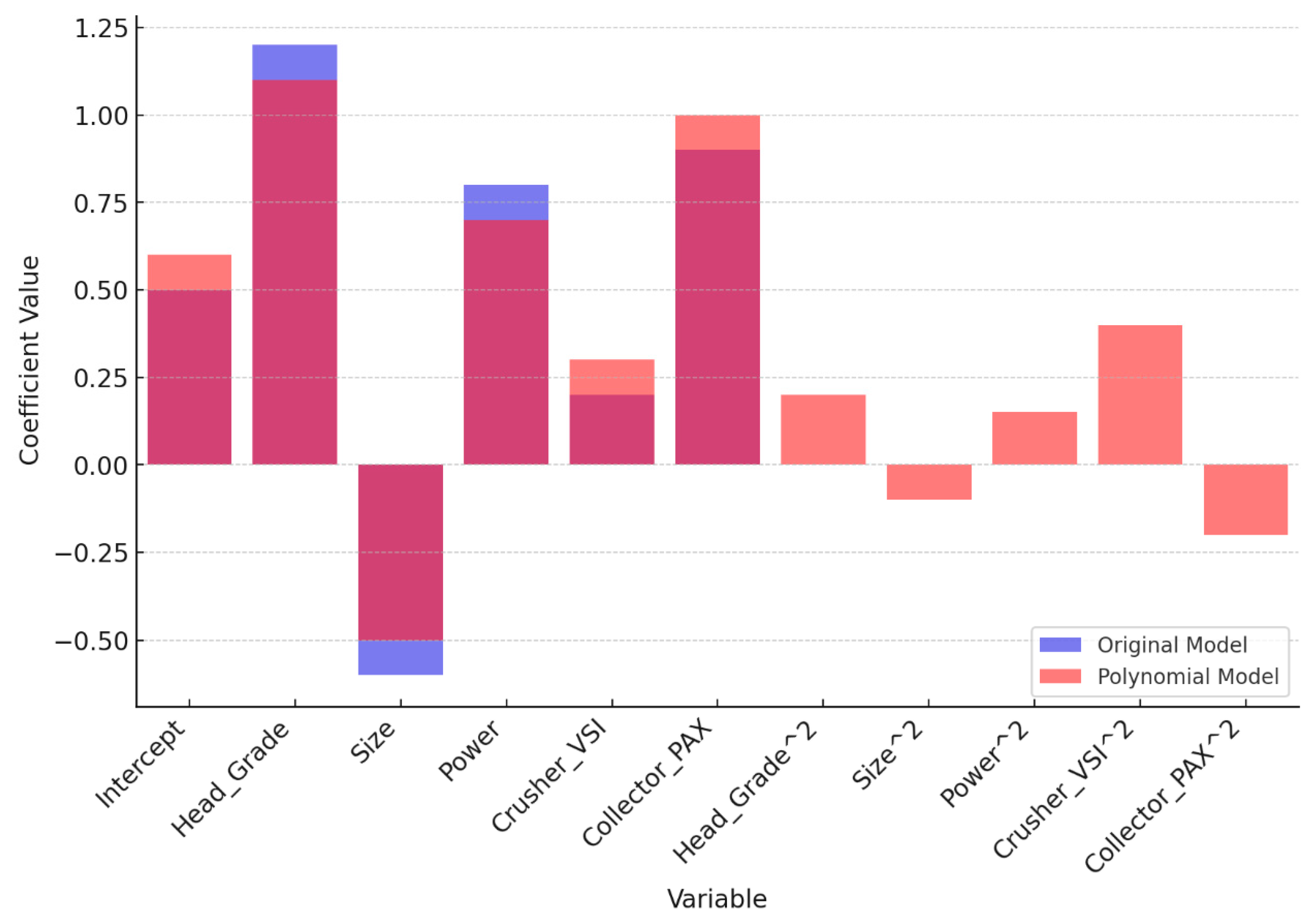
| Variable | Original Model | Polynomial Model |
|---|---|---|
| Head Grade (g/t) | Strong positive coefficient, narrow HDI, high ESS, ≈ 1 | Still dominant; Head_Grade2 introduces curvature with wider uncertainty |
| Size (mm) | Moderate negative coefficient, stable estimate | Size2 amplifies non-linearity; higher variance suggests overfitting |
| Power (kW) | Moderate positive influence | Power2 term significant; more flexible but greater uncertainty |
| Crusher_VSI | Marginal impact; HDI includes zero | Crusher_VSI2 shows impact, but interpretability suffers due to variance |
| Collector_PAX | Positive effect, reasonable confidence bounds | Collector_PAX2 inflates variance, suggesting instability |
Disclaimer/Publisher’s Note: The statements, opinions and data contained in all publications are solely those of the individual author(s) and contributor(s) and not of MDPI and/or the editor(s). MDPI and/or the editor(s) disclaim responsibility for any injury to people or property resulting from any ideas, methods, instructions or products referred to in the content. |
© 2025 by the author. Licensee MDPI, Basel, Switzerland. This article is an open access article distributed under the terms and conditions of the Creative Commons Attribution (CC BY) license (https://creativecommons.org/licenses/by/4.0/).
Share and Cite
Devasahayam, S. Advancing Flotation Process Modeling: Bayesian vs. Sklearn Approaches for Gold Grade Prediction. Minerals 2025, 15, 591. https://doi.org/10.3390/min15060591
Devasahayam S. Advancing Flotation Process Modeling: Bayesian vs. Sklearn Approaches for Gold Grade Prediction. Minerals. 2025; 15(6):591. https://doi.org/10.3390/min15060591
Chicago/Turabian StyleDevasahayam, Sheila. 2025. "Advancing Flotation Process Modeling: Bayesian vs. Sklearn Approaches for Gold Grade Prediction" Minerals 15, no. 6: 591. https://doi.org/10.3390/min15060591
APA StyleDevasahayam, S. (2025). Advancing Flotation Process Modeling: Bayesian vs. Sklearn Approaches for Gold Grade Prediction. Minerals, 15(6), 591. https://doi.org/10.3390/min15060591