Research and Application of 3D Magnetic Inversion Method Based on Residual Convolutional Neural Network

Abstract

Although various magnetic inversion techniques have been developed in geophysics, traditional methods are often constrained by inherent limitations such as low computational efficiency and pronounced non-uniqueness. In 3D magnetic inversion, multi-dimensional deep learning methods have shown promise in numerical simulations; however, their generalization capabilities and practical effectiveness in real-world geological applications, particularly in complex settings like gold exploration, remain underexplored. This study introduces MAGNETPRO, a residual convolutional neural network based on an encoder–decoder architecture, designed to accurately invert 2D magnetic field data into 3D magnetic susceptibility structures. To enhance the model’s generalization ability and inversion accuracy, an innovative data construction strategy was implemented to create a highly randomized training dataset incorporating complex geological features. Theoretical model tests demonstrate that MAGNETPRO achieves inversion accuracies of 97% across the entire region and 80% within magnetic structure areas, highlighting its excellent spatial resolution and structural recognition capabilities. To further validate its practical effectiveness, the method was applied to real exploration data from a gold mining area in Fujian Province. The results show a high degree of consistency between the inversion outcomes and drilling data, confirming the method’s reliability and practical value under real geological conditions.

1. Introduction

As one of the fundamental methodologies in geophysical exploration, magnetic surveying plays a pivotal role in mineral resource investigations, particularly in the detection of metal ores such as iron and copper. Through inversion of magnetic anomaly data, subsurface magnetic susceptibility distributions can be reconstructed to quantitatively characterize ore body geometry, depth, and spatial dimensions, thereby providing critical constraints for mineral exploration [1]. Recent advancements in geophysical inversion techniques have established three-dimensional (3D) inversion as the standard approach for quantitative interpretation of potential field data. Theoretical and practical studies have demonstrated that appropriately designed objective functions can effectively resolve complex geological structures [2]. However, the inherent quadratic attenuation of magnetic field intensity with source distance results in rapid signal decay for deep-seated anomalies, leading to diminished depth resolution and pronounced non-uniqueness in inversion solutions—a persistent challenge in magnetic data interpretation.

To address these limitations, multiple strategies have been proposed, including depth weighting constraints and integration of multi-source datasets (e.g., gradient tensor data acquired through varied instrumentation) [3,4,5,6,7,8,9,10,11,12]. While these approaches have demonstrated varying degrees of success in mitigating depth resolution issues, their practical implementation remains constrained by geological complexity and data acquisition limitations. Of particular concern is the critical dependence of linear inversion schemes on initial model selection, which frequently leads to convergence at local minima and compromises computational stability—a significant drawback in scenarios where reliable a priori geological information is unavailable.

The advent of machine learning (ML), particularly deep learning (DL), has revolutionized the framework for solving ill-posed inverse problems in geophysics. As a subset of ML, DL employs hierarchical neural architectures to autonomously extract high-level features from raw data, circumventing the labor-intensive feature engineering required in conventional methods. Deep neural networks (DNNs), the cornerstone of DL, have demonstrated exceptional capability in processing large-scale geophysical datasets through unsupervised or semi-supervised learning paradigms. Recent applications in potential field inversion highlight DNNs’ proficiency in reconstructing subsurface structures from magnetic and gravity data with enhanced precision and computational efficiency.

Building upon these developments, innovative DL architectures have emerged for magnetic inversion. Zhang et al. [13] implemented an end-to-end magnetic susceptibility mapping framework (MagInvNet) using a U-Net architecture, while Mukherjee et al. [14] achieved significant improvements in resolution and efficiency through convolutional neural networks (CNNs) operating on unstructured meshes. Subsequent studies by Deng et al. [15] and Jia et al. further advanced the field through CNN-based geometric feature extraction and encoder–decoder architectures for 3D susceptibility modeling, respectively.

Despite these advancements, current DL implementations exhibit limited generalizability when confronted with weak magnetic anomalies in complex geological settings. This study presents a novel framework combining generalizable training strategies with optimized feature extraction networks to achieve high-precision 3D magnetic inversion. Our methodology specifically addresses the challenges of weak anomaly resolution through two key innovations: (1) Various methods, such as residual connections, skip connections, and adjustments to network architecture parameters, are employed to optimize network performance; (2) A large number of training samples with prominent generalization features are utilized. The proposed approach demonstrates superior performance in resolving subtle magnetic signatures compared to conventional and existing DL-based methods, as validated through synthetic benchmarks and field applications in metal exploration.

2. Methodological Framework

2.1. Training Sample Generation Protocol

The forward modeling process initiates with discretizing the subsurface medium into a regular grid of cuboidal cells, where each cell possesses homogeneous magnetic properties. For each cuboidal element, the analytical expressions governing its magnetic anomaly field are derived through closed-form solutions [16]. These fundamental equations form the mathematical basis for synthetic data generation:

$$\Delta T\left(x,y,z\right)={\displaystyle \frac{u_{0}J}{4\pi }}\left[\begin{array}{l}-K_1\arctan {\displaystyle \frac{\xi }{\eta +\zeta +R}}-K_2\arctan {\displaystyle \frac{\eta }{\xi +\zeta +R}}+\\ K_3\arctan {\displaystyle \frac{\xi +\eta +R}{\zeta }}+K_4\ln (\xi +R)+\\ K_5\ln (\eta +R)+K_6\ln (\zeta +R)\end{array}\right]\left|\begin{array}{l}{\xi }_2-x\\ {\xi }_1-x\end{array}\right.\left|\begin{array}{l}{\eta }_2-y\\ {\eta }_1-y\end{array}\right.\left|\begin{array}{l}{\zeta }_2-z\\ {\zeta }_1-z\end{array}\right.$$

(1)

where $\left(x,y,z\right)$ is the coordinate of the grid point on the observation plane; $\left(\xi ,\eta ,\zeta \right)$ is the coordinate of the source point of the rectangular body, and its corresponding integration limit changes in the range of $\left({\xi }_1,{\xi }_2\right), \left({\eta }_1,{\eta }_2\right),\left({\zeta }_1,{\zeta }_2\right)$; $R=\sqrt{{\xi }^2+{\eta }^2+{\zeta }^2}$; J is the total magnetization intensity of the rectangular prism; ${\mu }_0$ is the magnetic permeability in the vacuum; $K_1=2Ll$; $K_2=2Mm$; $K_3=2Nn$; $K_4=Nm+Mn$; $K_5=Nl+Ln$; $K_6=Ml+Lm$; and $l,m,n$ and $L,M,N$ are the cosine of the direction of the geomagnetic field and the total magnetization intensity, respectively.

The computational complexity of forward modeling exhibits linear scaling with both observation points (N_d) and model discretization units (N_m) [17]. This scaling relationship introduces two critical bottlenecks: (1) sensitivity matrix operations requiring O (N_d × N_m) floating-point computations, (2) memory-intensive matrix–vector multiplications. Conventional CPU-based implementations face severe performance degradation when addressing large-scale 3D aeromagnetic modeling scenarios, particularly in continental-scale surveys exceeding 10⁶ measurement points.

Recent advances in heterogeneous parallel computing architectures (CPU/GPU) have demonstrated order-of-magnitude acceleration in potential field modeling [18,19,20,21]. Building on these developments, our framework achieves fast orthogonal computation of sample set models through the following optimizations:

2.1.1. Memory-Efficient Sensitivity Handling

Exploiting the embarrassingly parallel nature of sensitivity matrix elements, we implement row/column-wise distributed computing with dynamic memory allocation:

• Row-parallel mode: Computes magnetic contributions from all model units to individual measurement points.
• Column-parallel mode: Calculates the influence of single model units across all measurement points.

The superposition principle is then applied through parallel reduction operations, reducing peak memory consumption by 58% compared to full-matrix storage.

2.1.2. Sparse Matrix Optimization

Since most of the background susceptibility perturbations in the model are zero (92%), the sensitivity matrix becomes a large, sparse matrix. Before calculating the magnetic anomaly, a mask can be applied to block out the zero elements in the sensitivity matrix, so that only the nonzero elements are computed, thereby further reducing computational load and memory requirements, and improving computational efficiency.

$$G_{\mathrm{sparse}}=G\odot M\left({\kappa }_{\mathrm{threshold}}\right)$$

(2)

where $M$ denotes the susceptibility-dependent binary mask. $G_{\mathrm{sparse}}$ represents the sparse version of the matrix or vector $G$. $G$ is the original matrix or vector. $\odot$ denotes element-wise multiplication (Handmard product). $M\left({\kappa }_{\mathrm{threshold}}\right)$ is a susceptibility-dependent binary mask, where the mask is generated based on the threshold parameter ${\kappa }_{\mathrm{threshold}}$.

This sparsification reduces non-zero matrix elements by 63% ± 8% across test cases, effectively transforming the problem into a Compressed Sparse Row (CSR) format computation.

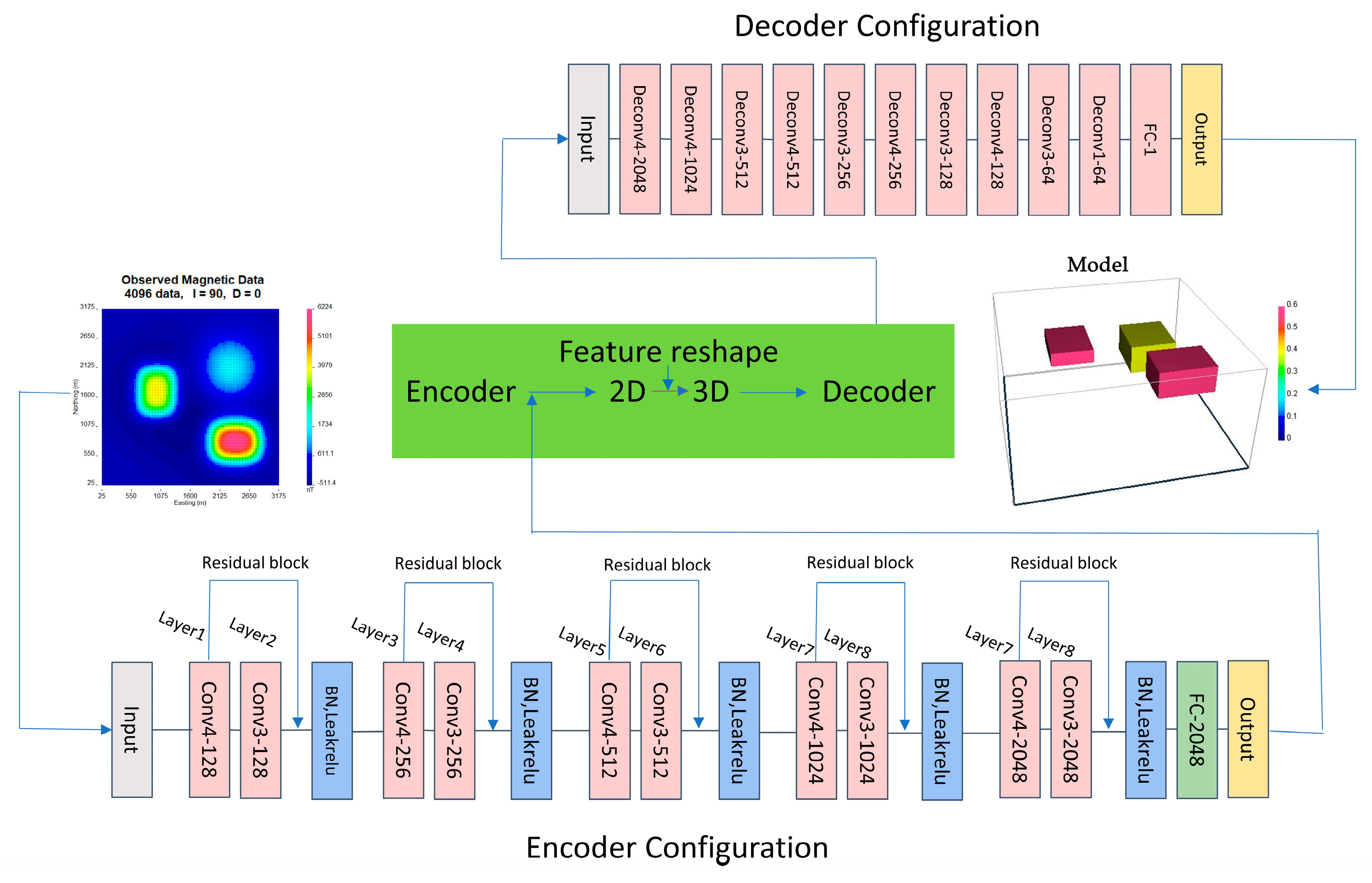
2.2. Based on Convolutional Neural Networks

In the era of artificial intelligence, it is particularly critical to develop efficient and high-precision inversion algorithms. Drawing on the outstanding performance of deep learning in nonlinear mapping, this paper proposes a three-dimensional magnetic inversion method based on the deep learning framework and constructs an end-to-end deep neural network structure. The network is trained by using a highly random sample of data that can characterize complex underground susceptibility structures and is ultimately used for inversion prediction. The entire network structure consists of three parts: the encoder, the 3D converter, and the decoder. The input data are magnetic anomaly data on the observation plane, and the magnetic anomaly data are processed into a two-dimensional image as input to the network, while the known underground susceptibility model is used as training labels [17]. By supervising the learning of the convolutional neural network, the trained model is finally used to invert and predict the actual measured magnetic anomaly data.

In magnetic inversion, it can be considered that a complete three-dimensional magnetic susceptibility structure is deconstructed through a compressed projection magnetic susceptibility structure, that is, a magnetic susceptibility structure containing relatively complete horizontal information and vertical information after compression distortion. The refactoring function r is defined as:

$${\mathit{m}}_{3d}=r\left({\mathit{m}}_{2d}\right)$$

(3)

where ${\mathit{m}}_{2d}$ is a two-dimensional magnetic susceptibility structure and ${\mathit{m}}_{3d}$ is a three-dimensional magnetic susceptibility structure.

The two-dimensional feature used for reconstruction by magnetic inversion is position field information. The inversion function i is defined as:

$${\mathit{m}}_{2d}=i\left({\mathit{d}}_{2d}\right)$$

(4)

The three-dimensional susceptibility inversion function can be constructed as a functional of the above two functions, expressed as:

$$\mathit{m}=f\left(\mathit{d}\right)=r\left(i\left(\mathit{d}\right)\right)$$

(5)

When training predictions, neural networks unify the implementation of the two functions into direct learning of three-dimensional inversion functions f.

This study proposes a magnetic anomaly inversion method based on deep learning, solves the problem of dimension mismatch between two-dimensional magnetic anomaly data and three-dimensional magnetic atomicity model, and innovatively designs a three-dimensional dimension converter. As the output layer of the network, the converter can effectively map the two-dimensional feature map to the three-dimensional space. The network model first extracts the characteristics of two-dimensional magnetic anomaly data through sampling, and then expands the output two-dimensional data, thereby achieving the precise description of the physical properties of underground three-dimensional magnetic bodies. Through end-to-end training, the model can directly invert the three-dimensional magnetic susceptibility structures from the two-dimensional magnetic anomaly data, greatly improving the efficiency and accuracy of the inversion, and achieving the goal of end-to-end inversion prediction (as shown in Figure 1).

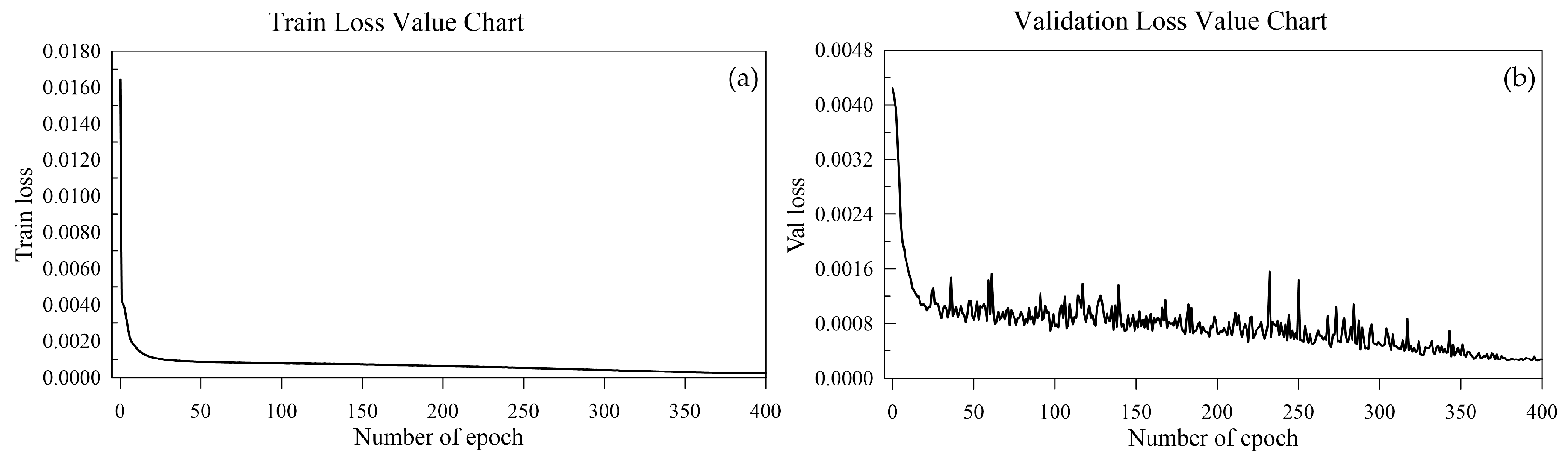
2.3. Training and Evaluation Metrics for Neural Networks

Building upon recent advances in deep learning-based inversion [22,23,24], the mean squared error (MSE) loss is employed to address the optimization problem (Equation (6)). The accuracy of the 3D magnetic inversion results is evaluated using Equations (7)–(9).

$${\mathrm{MSE}}_{\mathrm{Loss}}={\displaystyle \frac{1}{n}}{\displaystyle \sum _{i=1}^n{(m_i^{*}-m_i)}^2}$$

(6)

$$\mathrm{MAE}={\displaystyle \frac{1}{n}}{\displaystyle \sum _{i=1}^n}|m_i^{*}-m_i|$$

(7)

$$E_{\mathrm{acc}}=|m_i^{*}-m_i|<r$$

(8)

$$N_{acc}=max((m_i^{*}/m_i),(m_i/m_i^{*}))<t$$

(9)

where $m_i^{*}$ represents the true value, $m_i$ is the predicted value. r is the preset threshold for absolute difference (set to r = 0.01 in this paper), and t is the preset threshold for ratio (set to t = 1.20 in this paper); both are dimensionless. MSE_Loss (mean squared error loss) is used as the loss function. MAE (mean absolute error) represents the average absolute error. E_acc denotes the accuracy over the entire grid region, while N_acc refers to the accuracy within the anomalous region.

A grid cell is considered accurately predicted in E_acc if the absolute difference between $m_i^{*}$ and $m_i$ is smaller than the threshold r. E_acc is calculated as the number of accurately predicted grid cells divided by the total number of grid cells.

For N_acc, a grid cell is considered accurately predicted if the maximum of the ratio between $m_i^{*}$ and $m_i$ (or vice versa) is less than the threshold t. N_acc is computed as the number of accurately predicted grid cells divided by the total number of anomalous grid cells.

2.4. Building a Dataset

To meet the requirements of deep learning geophysical inversion methods for dataset size and diversity, a three-dimensional magnetic inversion dataset (MagInv) was constructed. It contains 80,000 sets of three-dimensional magnetic susceptibility models and their corresponding two-dimensional magnetic field anomaly data. The construction process of the data set mainly includes two steps: model design and forward simulation.

To ensure the representativeness of the data set, seven types of sample models were designed, including single block, combined block, single step, combined step, single block and step combination, complex block and step combination, and step combinations containing heterogeneous blocks (

Table 1. Comparison table of design methods and parameters of various magnetic models.

Model Type	Design Parameters	Magnetic Susceptibility Settings
Single Block	Horizontal coordinates of SW corner: Select one of the 48 meshes from the center randomly Horizontal mesh length: 8–24 Depth of top interface: 2–16 Vertical mesh length: 2–16	0.01~1 SI, with an interval of 0.01
Combined Block	Number of blocks: 3–7 Horizontal coordinates of SW corner: Select one of the 48 meshes from the center randomly Horizontal mesh length: 8–24 Depth of top interface: 2–10 Vertical mesh length: 2 + (random number between 1 and top burial depth)	0.01~1 SI, with an interval of 0.01
Single Step	Horizontal coordinates of SW corner: Select one of the 60 meshes from the center randomly Horizontal mesh length: 3–16 Depth of top interface: 1–10 Vertical mesh length: 5–54 Thickness of each step: 1–3 Horizontal dislocation distance for each step: 1–3	0.01~1 SI, with an interval of 0.01
Combined Step	The same as the single step.	0.01~1 SI, with an interval of 0.01
Combination of Single Block and Step	The same as the single block and the single step.	0.01~1 SI, with an interval of 0.01
Combination of Complex Block and Step	The same as the single block and the single step.	0.01~1 SI, with an interval of 0.01
Combination of Step with Heterogeneous Block	Add multiple small blocks or steps around the block or step model of a certain scale.	0.01~1 SI, with an interval of 0.01

). Each type of model is further sub-typed, covering the variations of various factors such as horizontal distribution, burial depth, size, and physical properties [25]. Finally, a total of 80,000 model samples were generated and divided into training sets, validation sets and test sets at a ratio of 3:1:1. Among them, the training set contains 48,000 samples, and the validation set and the test set each contain 16,000 samples. The training process was conducted on a Lenovo workstation (Beijing, China) equipped with an Intel i7-11370H CPU, 64 GB of RAM, and dual NVIDIA GeForce RTX 3060 GPUs (12 GB each). Each training epoch required approximately 33 min, resulting in a total training time of about 220 h.

Employing the forward modeling method (Equation (1)) from the previously described numerical simulation framework, the designed model is used to generate two-dimensional magnetic anomaly field data through forward simulation. These data are used as input to the neural network and to train the model together with the corresponding model parameters (labels). To simulate underground structures, a fixed Cartesian meshing method is used in this paper. The model is divided into 64, 64, and 32 grid units in the x (east), y (north), and z (vertical) directions, respectively. The grid spacing is set to 50 m, and the coordinate origin is set to the southwest corner (0, 0, 0). The observation network consists of 4096 measurement points, with both point and line spacing set to 50 m. The southwest corner (25, 25) is the starting observation point, and all measurement points are located at the center of the corresponding grid cell. All coordinate units in the images involving magnetic forward models, forward magnetic fields, and inversion results in this article are in meters (m) and will not be described below.

Training datasets of varying sizes, ranging from 4000 to 48,000 samples, were tested, and the same test set was used for evaluation (

Table 2. Comparison of different numbers of the training dataset.

Evaluation Area	Evaluation Metric	4000	8000	16,000	24,000	32,000	40,000	48,000
Full Grid Region	MAE (10−3)	11.03	3.76	2.82	2.42	2.35	2.30	2.26
	Eacc (r = 0.01)	92.35	95.08	96.50	96.52	96.55	96.56	96.53
Anomalous Grid Area	MAE (10−2)	23.34	9.57	8.52	7.93	7.30	6.88	6.16
	Nacc (t = 1.2)	26.09	67.31	72.97	76.01	78.97	79.51	79.59

). As the size of the training data increased, the network exhibited improved performance, particularly in terms of inversion accuracy within the anomalous body regions, which showed significant enhancement.

The training and validation error curves in Figure 2 show a clear downward trend as the number of training epochs increases, indicating that the model is gradually learning the data features. After approximately 50 epochs, both error curves begin to stabilize. The validation error decreases rapidly during the initial stages and then plateaus, demonstrating good generalization performance on unseen data. These training results indicate that the proposed inversion model and network training strategy are effective and appropriately designed.

The MagInv dataset designed in this article has the following characteristics:

Large size: It contains 80,000 model samples, providing sufficient training data for deep learning models.

High diversity: It includes a wide range of model types that reflect the complexity of real geological structures.

High quality: A mature forward modeling method is used for simulation, ensuring reliable data accuracy.

The MagInv dataset designed in this paper can be widely used in the field of three-dimensional inversion of magnetic methods, including training of deep learning models, algorithm evaluation, and practical applications. Using this dataset, the MAGNETPRO deep learning magnetic inversion neural network model was trained, enabling high-precision magnetic inversion. In the final actual regional application, this model is used to predict the actual area of a gold mine in Fujian, and the results obtained have a high degree of consistency with geological and mineral data.

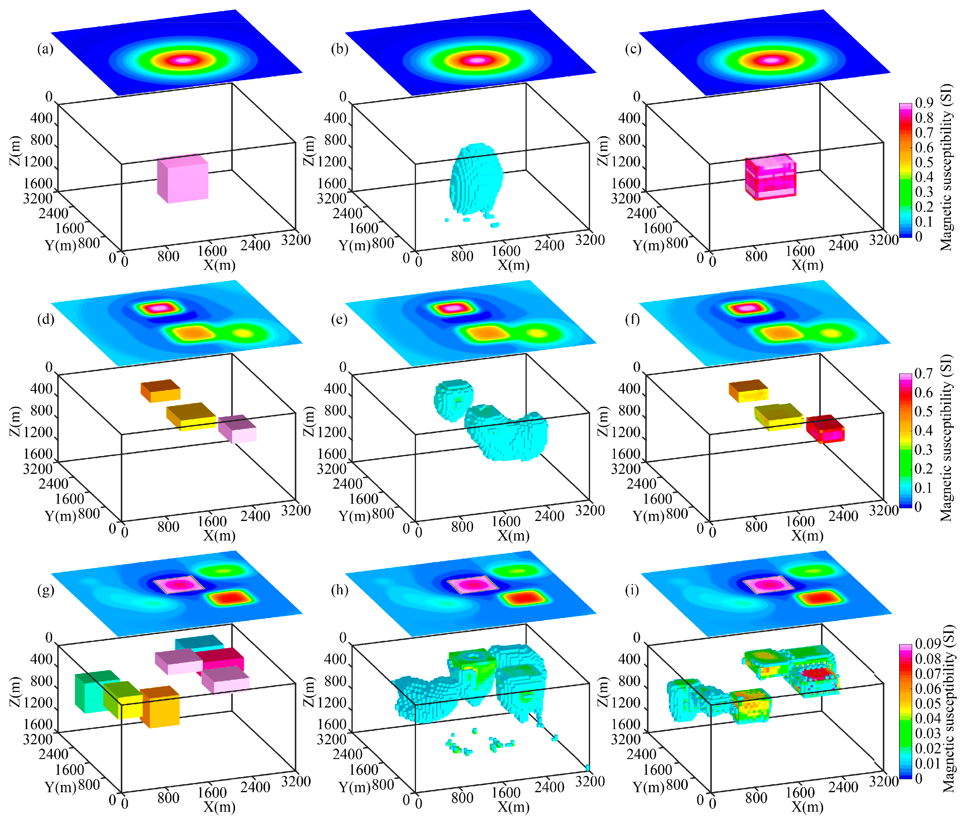
3. Theoretical Model Experiment

The labels and deep learning inversion results of the combined block model are shown in Figure 3. Figure 3a,d,g show the model magnetization labels. Figure 3b,e,h present the classical least squares inversion results. Figure 3c,f,i show the corresponding deep learning inversion results. Figure 3b,c highlight regions with magnetic susceptibility values above 0.6 (SI). In this case, the inversion accuracy (with threshold t = 1.20) reached 88%. Figure 3d illustrates three block models with different burial depths, shapes, and physical properties, having magnetic susceptibility values of 0.4 (SI), 0.5 (SI), and 0.7 (SI), respectively. Figure 3e,f show the inversion results for susceptibility values greater than 0.32 (SI), where blocks with medium and high susceptibility are visible, while low-susceptibility objects are not detected. Figure 3g includes seven blocks varying burial depths, shapes, and physical properties, with the magnetic susceptibility from low to high in order of 0.01 (SI), 0.02 (SI), 0.04 (SI), 0.06 (SI), 0.08 (SI), 0.09 (SI). Figure 3h,i show the inversion results for susceptibility values greater than 0.01 (SI). In addition to the slightly inaccurate prediction of the edges of some geological bodies, the distribution of underground magnetic susceptibility is depicted more accurately overall. The buried depth and shape of the seven blocks are clearly distinguished, and have good resolution in the horizontal and vertical directions, and the difference in magnetic susceptibility is also accurately identified. The inversion accuracy (t = 1.20) of the anomaly grid area reached 85%. In terms of computation time, classical inversion took approximately 76 s, while the deep learning inversion required only 0.5 s, significantly improving inversion efficiency. These results demonstrate that deep learning inversion can accurately resolve burial depth, volume, and physical properties of composite models, offering great potential for high-precision geological modeling and interpretation.

As illustrated in the figure, both classical and deep learning inversions achieve good horizontal resolution. However, as the model complexity increases, the classical method struggles to resolve the boundaries of adjacent anomalous bodies, with recovered physical parameters showing significant deviations from the true model. In contrast, deep learning inversion provides clearer delineation of burial depth and geometry, although inaccuracies persist at the edges of some anomalies. In physical property recovery, deep learning also presents deviations: models with higher magnetization tend to show reduced magnetization values after inversion, while models with lower magnetization show slight increases. In particular, neither classical nor deep learning inversion captures extremely low-magnetization anomalies between adjacent models with large magnetization contrasts (e.g., 0.09 and 0.01). Nevertheless, for isolated anomalous bodies with relatively low magnetization (e.g., 0.02), deep learning inversion maintains clear boundary definition without significant interference from surrounding structures. Overall, deep learning inversion outperforms the classical method in physical property recovery, enabling more accurate characterization of burial depth, volume, and physical properties. These results demonstrate the great potential of deep learning inversion for high-precision geological modeling and interpretation.

4. Application Examples

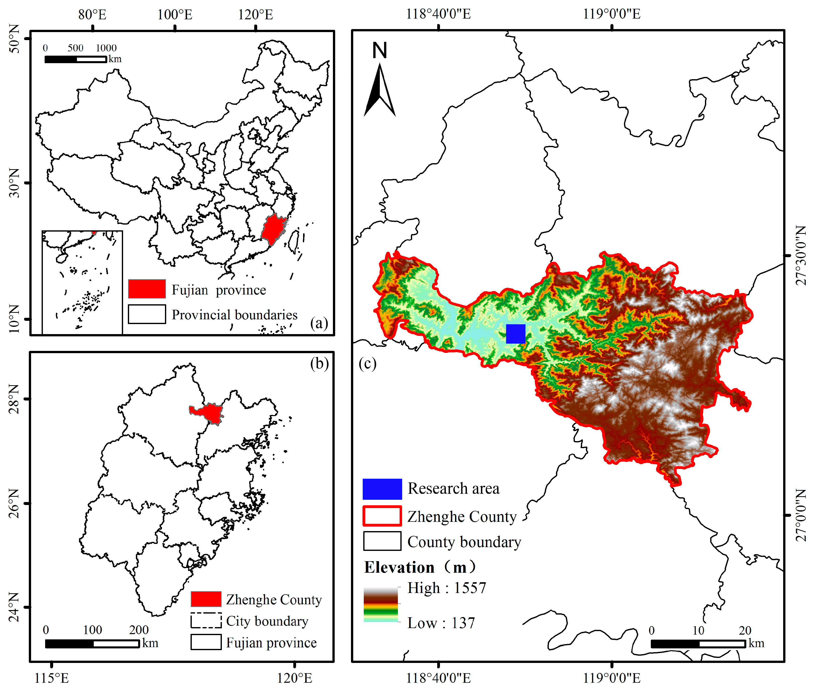
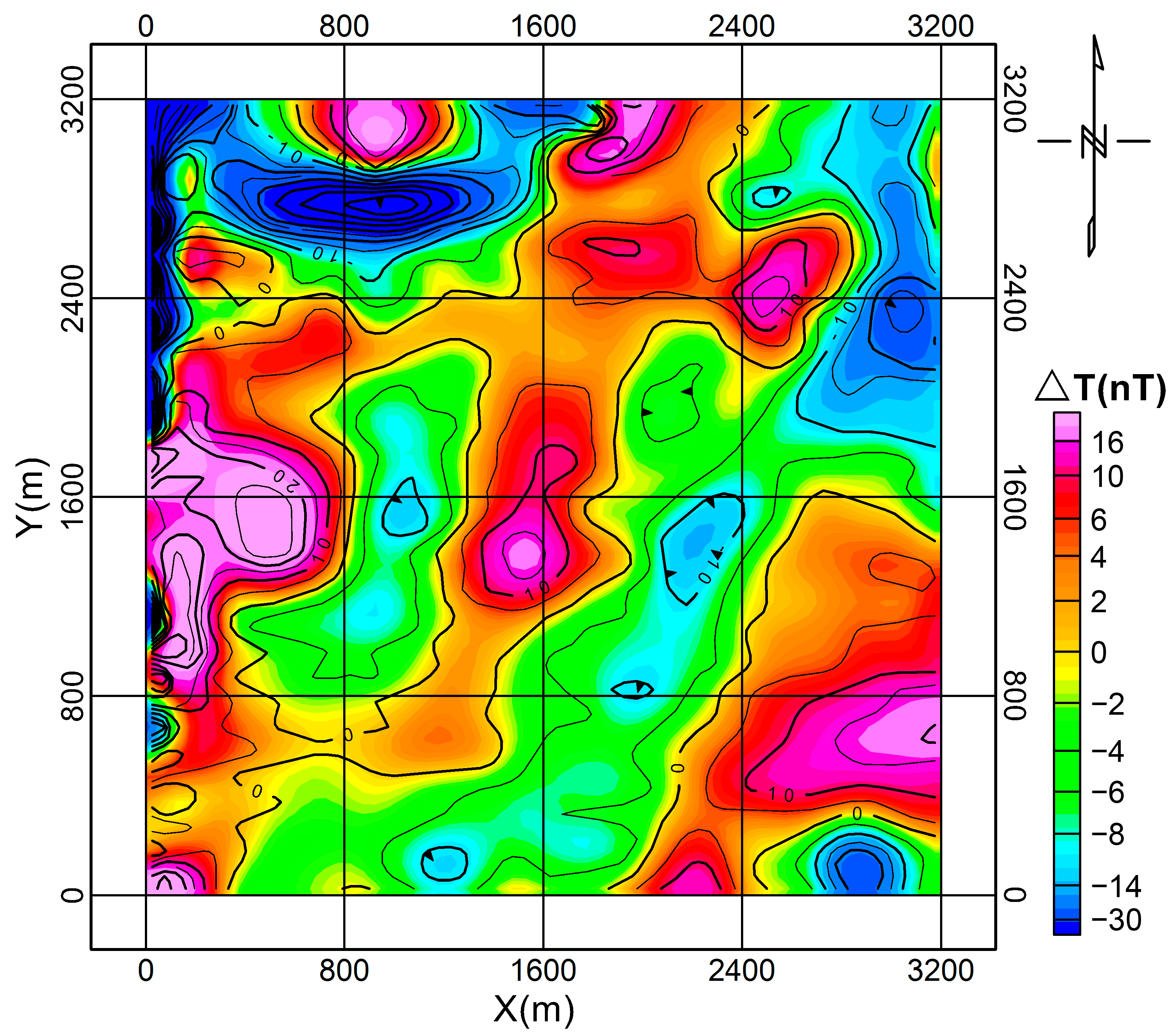
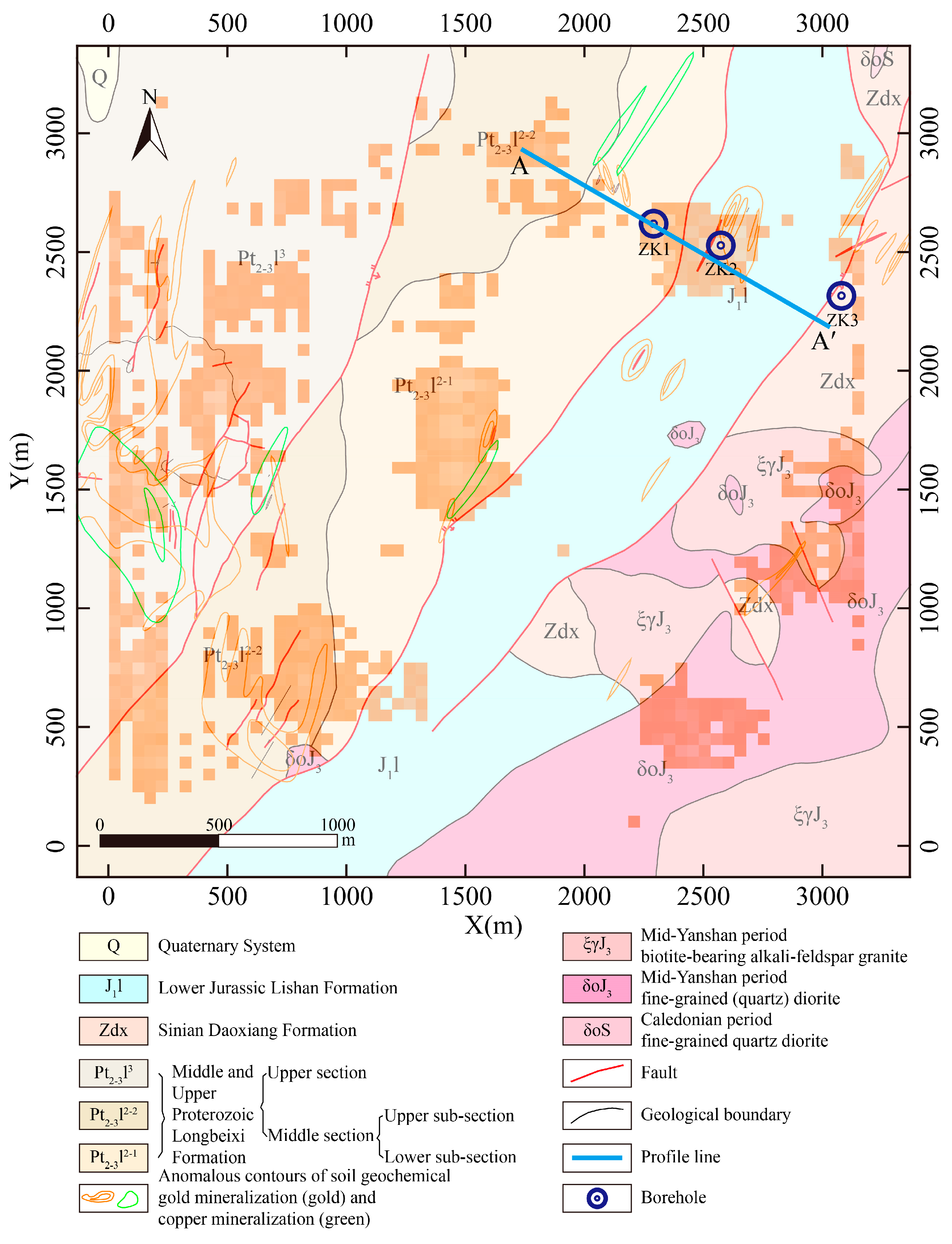
4.1. Geological Background

The research area is located at the junction of Fujian and Zhejiang, in Northern Fujian Province (Figure 4), and belongs to the middle and low hilly areas of the southeast coast. The basic morphology of the research area was shaped during the Yanshan movement, approximately 1 to 1.4 million years ago, with the fault activities during this period having a significant impact on the geomorphological features. The terrain in this area is higher in the east and lower in the west, with significant surface erosion, diverse landform types, and well-ordered layered arrangements. The main terrain units consist of extensive mountainous areas, narrow plains, and valleys, which can be classified into medium and low mountainous land, high and low hills, valleys, basins, and plains.

The research area is located in the Wuyi Mountain metallogenic belt, one of the key polymetallic mineralization regions in Fujian Province. The area’s structure is complex, formed by multiple stages of tectonic activity. It mainly exhibits three major fault sets: northeast, northwest, and near-north–south. The area exposed is above a Precambrian metamorphic substrate, which is not integrated with the volcanic rocks that overlay the region from the Late Jurassic period.

Magmatic activity has been frequent in the area. From the Late Proterozoic to the Jurassic, ultramafic, basic, intermediate, and acidic rocks have successively formed. These rock masses are mostly distributed along the fault zone, which has played a significant role in the region’s mineralization.

Based on the measurement results of naturally occurring heavy sand and waterborne sediments within the 1:50,000-scale area, the study area and its surrounding regions exhibit overlapping anomalies of heavy sand, gold, and waterborne sediments. These anomalies are mainly characterized by polymetallic elements such as gold, silver, copper, lead, and zinc, with distributions closely related to regional geological structures, indicating promising prospects for mineral exploration. Additionally, pyrite in the region, as a major carrier of rare metals such as gold and silver, exhibits significant magnetic contrast with the surrounding rocks, providing favorable conditions for conducting magnetic surveys.

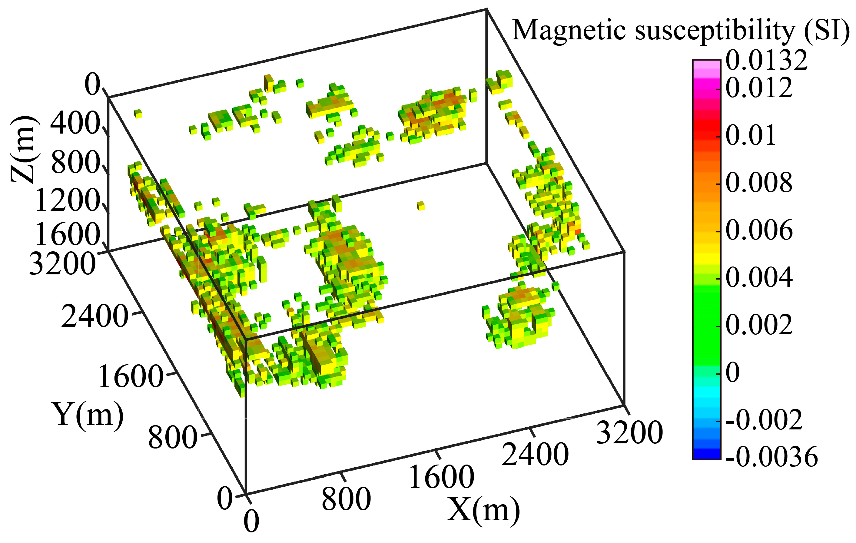
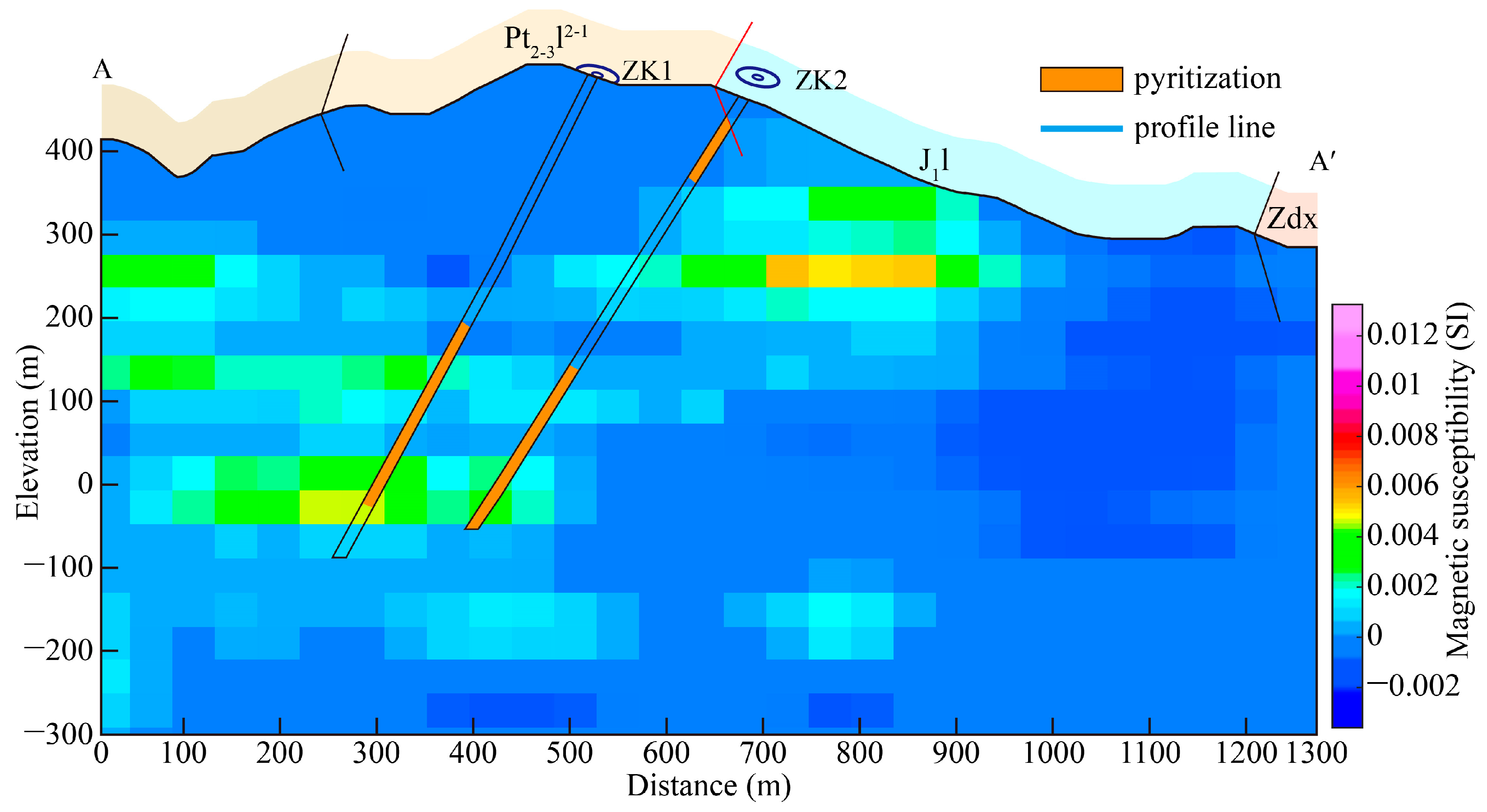
4.2. Results and Discussion

The magnetic survey lines were arranged based on the principle of being perpendicular to the main geological structures and regional gravity–magnetic anomalies of the study area, i.e., oriented in an east–west direction using a regular grid of 100 m × 20 m. The magnetic data were processed through diurnal variation correction, normal field correction, and field separation to obtain the ∆T magnetic anomaly (Figure 5).

From the contour map of the ∆T magnetic anomaly, it can be observed that a distinct magnetic anomaly belt is distributed throughout the study area, trending north–northeast and appearing as a string of beads along the trend. High-magnetic anomaly closures are present on the western side and in the southeastern part of the area.

The underground space in the research area is divided into grids, with 64, 64, and 32 cells in the x (east), y (north), and z (vertical) directions, respectively. The grid spacing is 50 m, and the starting coordinates at the southwest corner are (0, 0, 0). Figure 6 is a three-dimensional diagram showing areas with a magnetic susceptibility value greater than 0.003 (SI).

From Figure 6, it can be observed that the inversion anomalies reflect both the depth and planar position of the ore body. The inversion results indicate that the high-magnetic anomaly zone on the western side aligns well with the known ore body. Consequently, it is inferred that the high-magnetic anomaly areas in the central and northeastern regions may also correspond to gold-bearing mineralized zones.

To verify the accuracy of the inversion results, three boreholes were drilled in the northeastern part of the study area, based on the geological map and inversion results shown in Figure 7. The inversion results and borehole data were then combined and presented in Figure 8 (ZK3 is located at the edge of the study area, with the borehole dipping to the north. Its termination point extends beyond the study area; therefore, only ZK1 and ZK2 are shown.).

ZK1 intersected pyritization at depths of 45–217 m and 400–445 m;

ZK2 intersected pyritization at depths of 300–532 m;

ZK3 intersected pyritization at depths of 45–124 m, 300–490 m, and 502–563 m.

Laboratory analyses of core samples from ZK1, ZK2, and ZK3 show the following results: In ZK1, gold mineralization with a grade of 0.6 g/t was observed at 180 m, with the highest gold grade of 1.6 g/t and a silver grade of 5 g/t at 400 m. In ZK2, discontinuous mineralization was identified between 400 and 500 m, with a maximum gold grade of 0.6 g/t and a silver grade of 13 g/t. In ZK3, the gold grade at 155 m was 0.5 g/t, while the silver grade reached 32 g/t at 520 m.

5. Conclusions

Deep learning methodologies demonstrate superior precision in reconstructing the burial depth, geometry, and physical properties of subsurface anomalies. This study establishes two key innovations in magnetic inversion: (1) a residual-enhanced neural architecture enabling precise anomaly geometry reconstruction, and (2) a randomization-driven sampling strategy generating 80,000 synthetic models with comprehensive geological variability. These innovations collectively achieve 80% accuracy in magnetic target delineation, significantly outperforming conventional least-squares methods through enhanced nonlinear mapping.

Notable limitations persist: Amplitude recovery errors (particularly for weak anomalies) reveal incomplete physical learning, while finite training scenarios constrain generalization capacity. Future work should integrate adaptive learning mechanisms to bridge the gap between synthetic training and perfect field-data prediction. The framework, nevertheless, demonstrates transformative potential for addressing deep mineral exploration challenges through physics-aware deep learning.

References

1. Shamsipour, P.; Marcotte, D.; Chouteau, M. 3D stochastic joint inversion of gravity and magnetic data. J. Appl. Geophys. 2012, 79, 27–37. [Google Scholar] [CrossRef]
2. Oldenburg, D.W.; Li, Y. Inversion for applied geophysics: A tutorial. In Near-Surface Geophysics; Society of Exploration Geophysicists: Houston, TX, USA, 2005; pp. 89–150. [Google Scholar]
3. Pilkington, M. 3D magnetic data-space inversion with sparseness constraints. Geophysics 2009, 74, L7–L15. [Google Scholar] [CrossRef]
4. Chenot, D.; Debeglia, N. Three-dimensional gravity or magnetic constrained depth inversion with lateral and vertical variation of contrast. Geophysics 1990, 55, 327–335. [Google Scholar] [CrossRef]
5. Vitale, A.; Fedi, M. Inversion of potential fields with an inhomogeneous depth weighting function. In SEG Technical Program Expanded Abstracts 2019; Society of Exploration Geophysicists: Houston, TX, USA, 2019; pp. 1749–1753. [Google Scholar]
6. Shearer, S.; Li, Y. 3D inversion of magnetic total gradient data in the presence of remanent magnetization. In Proceedings of the SEG International Exposition and Annual Meeting, Denver, CO, USA, 10–15 October 2004; p. SEG-2004. [Google Scholar]
7. Wang, Y.; Rong, L.; Qiu, L.; Lukyanenko, D.V.; Yagola, A.G. Magnetic susceptibility inversion method with full tensor gradient data using low-temperature SQUIDs. Pet. Sci. 2019, 16, 794–807. [Google Scholar] [CrossRef]
8. Sanchez, V.; Sinex, D.; Li, Y.; Nabighian, M.; Wright, D.; vonG Smith, D. Processing and Inversion of Magnetic Gradient Tensor Data for Uxo Applications. In Proceedings of the 18th EEGS Symposium on the Application of Geophysics to Engineering and Environmental Problems, Atlanta, GA, USA, 3–7 April 2005; p. cp-183. [Google Scholar]
9. Nakagawa, I.; Yukutake, T.; Fukushima, N. Extraction of magnetic anomalies of crustal origin from Magsat data over the area of the Japanese Islands. J. Geophys. Res. Solid Earth 1985, 90, 2609–2615. [Google Scholar] [CrossRef]
10. Billings, S.D. Discrimination and classification of buried unexploded ordnance using magnetometry. IEEE Trans. Geosci. Remote Sens. 2004, 42, 1241–1251. [Google Scholar] [CrossRef]
11. Ma, G.; Wang, J.; Meng, Q.; Meng, Z.; Qin, P.; Wang, T.; Li, L. Research Develpment of Airborne Gravity (Magnetic) Multi-Components Gradient Detection and Inversion Technology. J. Jilin Univ. (Earth Sci. Ed.) 2023, 53, 1928–1949. [Google Scholar]
12. Ma, G.; Ma, S.; Li, L.; Cai, J. Method of self-structure-constrained inversion of magnetic anomalies and their magnetic gradients and its application in the exploration of coal burning area. Prog. Geophys. 2024, 39, 1026–1037. [Google Scholar] [CrossRef]
13. Zhang, Z.; Lu, R.; Liao, X.; Xu, Z.; Qiao, Z.; Fan, X.; Yao, Y.; Shi, Z.; Liu, P.; Lu, S. Inversion of magnetic anomaly and magnetic gradient anomaly based on fully convolution network. Prog. Geophys. 2021, 36, 325–337. (In Chinese) [Google Scholar]
14. Mukherjee, S.; Lelièvre, P.; Farquharson, C.; Adavani, S. Three-dimensional inversion of geophysical field data on an unstructured mesh using deep learning neural networks, applied to magnetic data. In Proceedings of the First International Meeting for Applied Geoscience & Energy, Denver, CO, USA, 26 September–1 October 2021; Society of Exploration Geophysicists: Houston, TX, USA, 2021; pp. 1465–1469. [Google Scholar]
15. Deng, H.; Hu, X.; Cai, H.; Liu, S.; Peng, R.; Liu, Y.; Han, B. 3D Inversion of Magnetic Gradient Tensor Data Based on Convolutional Neural Networks. Minerals 2022, 12, 566. [Google Scholar] [CrossRef]
16. Yao, L. Theoretical study on cuboid magnetic field and gradient expression without singular point. Oil Geophys. Prospect. 2007, 42, 714. (In Chinese) [Google Scholar]
17. Jia, Z.; Li, Y.; Wang, Y.; Li, Y.; Jin, S.; Li, Y.; Lu, W. Deep Learning for 3-D Magnetic Inversion. IEEE Trans. Geosci. Remote Sens. 2023, 61, 5905410. [Google Scholar] [CrossRef]
18. Chen, Z.; Meng, X.; Guo, L.; Liu, G. GICUDA: A parallel program for 3D correlation imaging of large scale gravity and gravity gradiometry data on graphics processing units with CUDA. Comput. Geosci. 2012, 46, 119–128. [Google Scholar] [CrossRef]
19. Tondi, R.; Cavazzoni, C.; Danecek, P.; Morelli, A. Parallel, ‘large’, dense matrix problems: Application to 3D sequential integrated inversion of seismological and gravity data. Comput. Geosci. 2012, 48, 143–156. [Google Scholar] [CrossRef]
20. Moorkamp, M.; Jegen, M.; Roberts, A.; Hobbs, R. Massively parallel forward modeling of scalar and tensor gravimetry data. Comput. Geosci. 2010, 36, 680–686. [Google Scholar] [CrossRef]
21. Chen, T.; Zhang, G. Forward modeling of gravity anomalies based on cell mergence and parallel computing. Comput. Geosci. 2018, 120, 1–9. [Google Scholar] [CrossRef]
22. Lin, Y.; Wu, Y. InversionNet: A real-time and accurate full waveform inversion with convolutional neural network. J. Acoust. Soc. Am. 2018, 144, 1683. [Google Scholar] [CrossRef]
23. Eigen, D.; Puhrsch, C.; Fergus, R. Depth map prediction from a single image using a multi-scale deep network. Adv. Neural Inf. Process Syst. 2014, 27, 2366–2374. [Google Scholar]
24. Eigen, D.; Fergus, R. Predicting depth, surface normals and semantic labels with a common multi-scale convolutional architecture. In Proceedings of the IEEE International Conference on Computer Vision, Santiago, Chile, 7–13 December 2015; pp. 2650–2658. [Google Scholar]
25. Zhang, L.; Zhang, G.; Liu, Y.; Fan, Z. Deep learning for 3-D inversion of gravity data. IEEE Trans. Geosci. Remote Sens. 2021, 60, 5905918. [Google Scholar] [CrossRef]
Figure 1. Schematic diagram of the structure and inversion process of the MAGNETPRO neural network.
Minerals 15 00507 g001
Figure 2. Training/validation error diagram. (a) Train loss curve and (b) validation loss curve.
Minerals 15 00507 g002
Figure 3. Comparison of deep learning inversion and classical inversion results for different models. (a,d,g) True models with varying magnetic susceptibilities; (b,e,h) Corresponding classical inversion results; (c,f,i) Corresponding deep learning inversion results.
Minerals 15 00507 g003
Figure 4. Traffic location map of a gold mine research area in Fujian. (a) Map of China showing the location of Fujian Province. (b) Map of Fujian Province showing the location of Zhenghe County. (c) Elevation map of Zhenghe County and location of the study area.
Minerals 15 00507 g004
Figure 5. Contour map of magnetic anomalies.
Minerals 15 00507 g005
Figure 6. Deep learning magnetization inversion (susceptibility value > 0.003 (SI)).
Minerals 15 00507 g006
Figure 7. Plan view of inversion results and geological map overlay.
Minerals 15 00507 g007
Figure 8. Comparison of drilled hole profiles (ZK1, ZK2 are boreholes).
Minerals 15 00507 g008