

The Joint Inversion of Seismic Ambient Noise and Gravity Data in an Ellipsoidal Coordinate System: A Case Study of Gold Deposits in the Jiaodong Peninsula
 , and
, and 
Abstract
1. Introduction
2. Methods
2.1. Forward Modeling in the Ellipsoidal Coordinate System
2.1.1. Gravity Anomaly
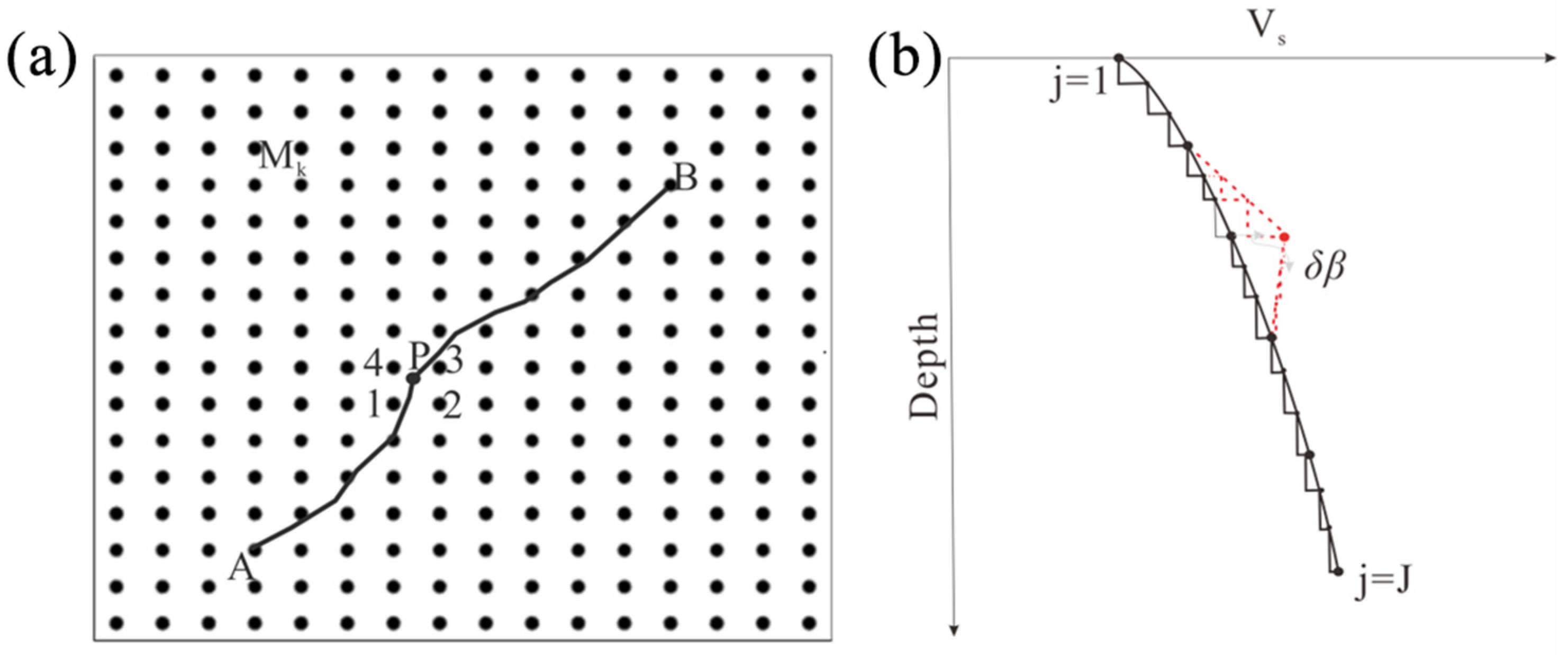
2.1.2. Seismic Data
2.2. Inversion Method
2.2.1. Single Inversion
2.2.2. Joint Inversion
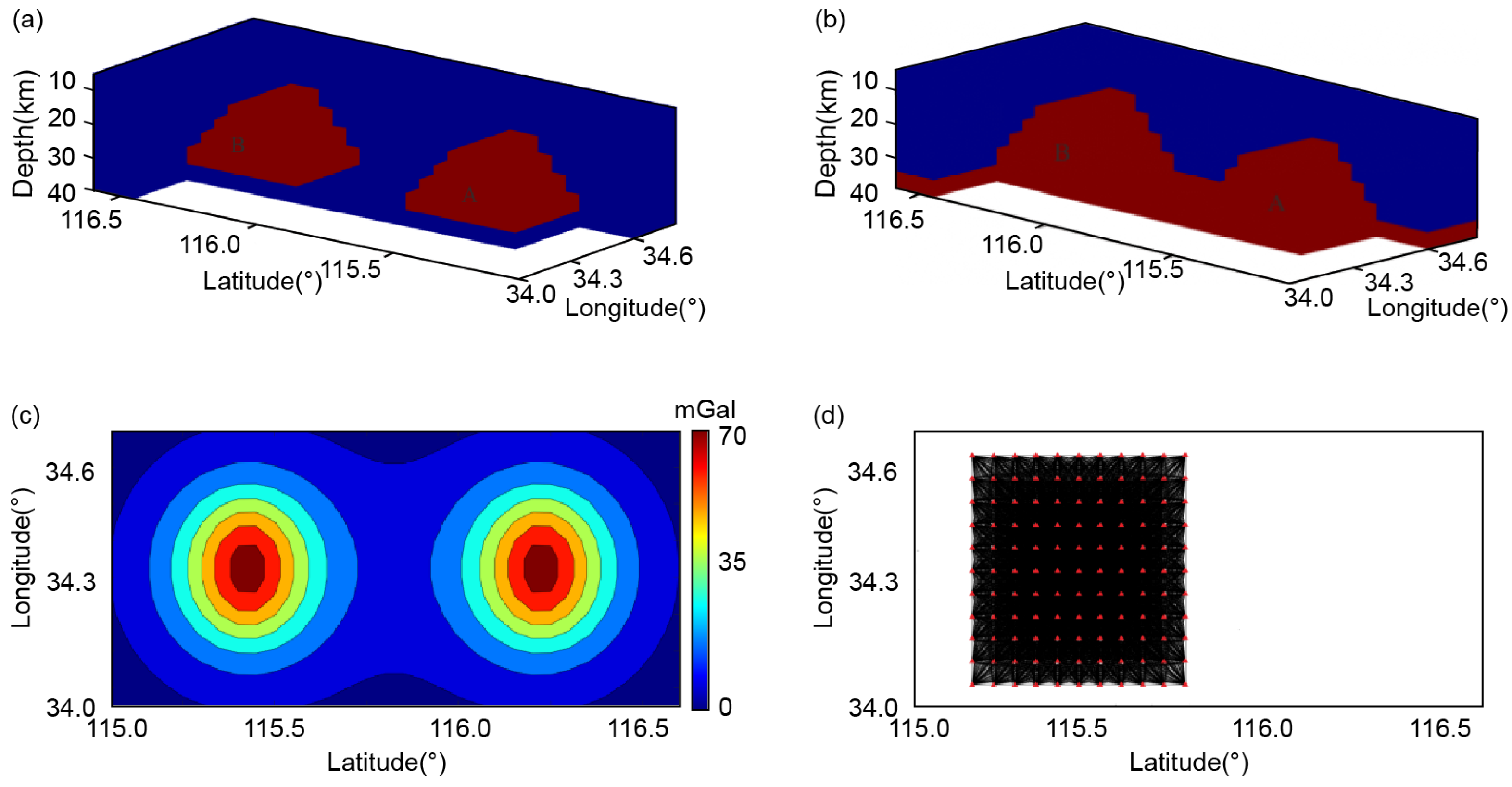
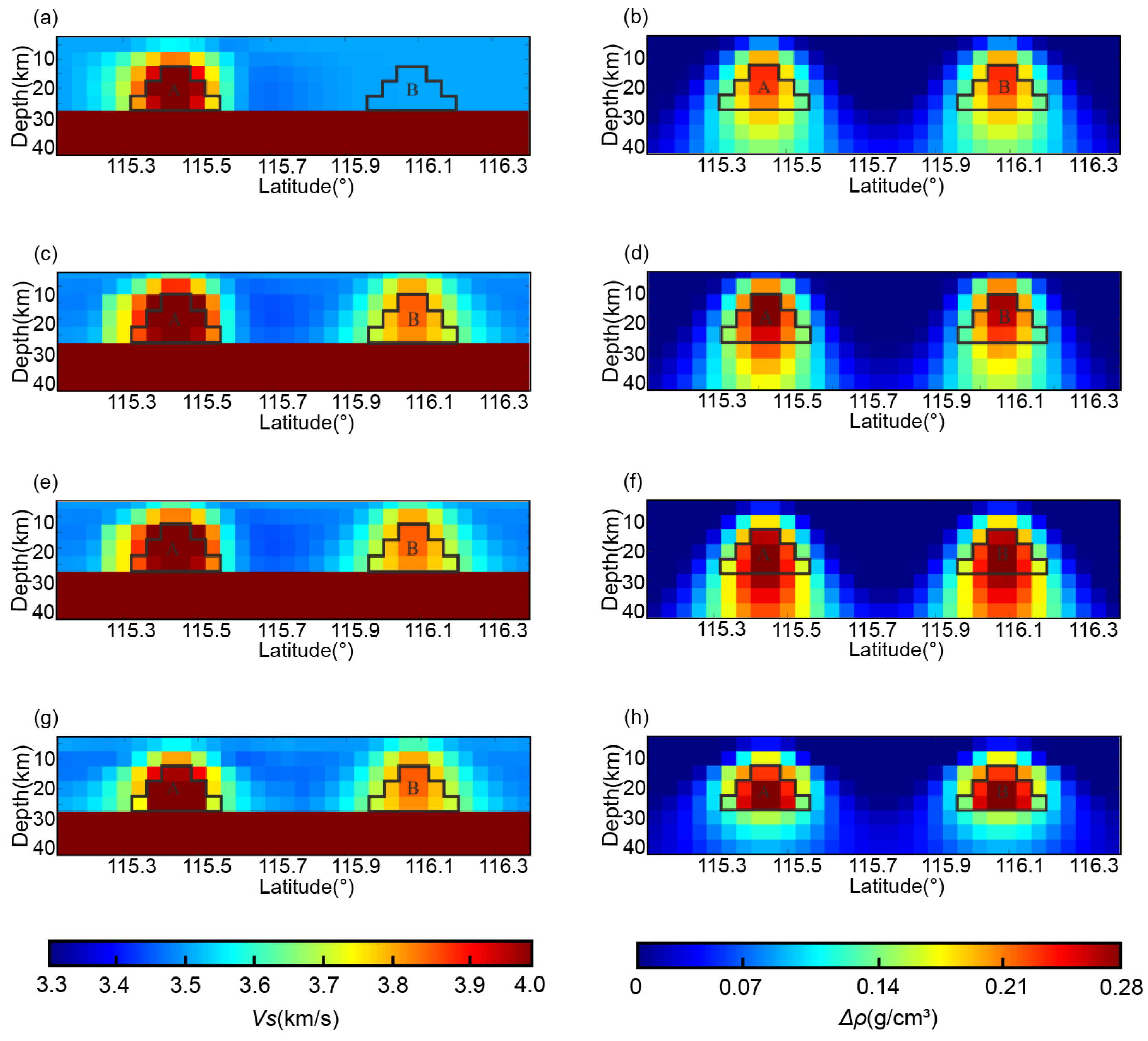
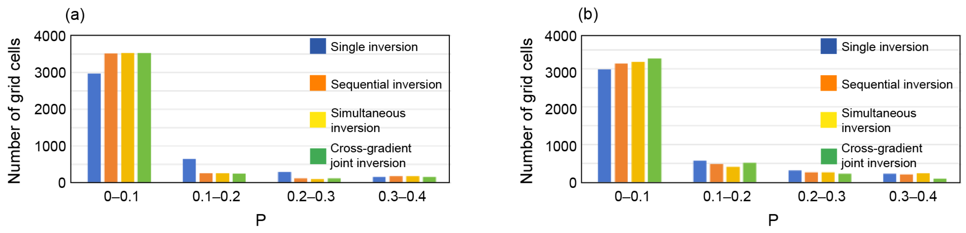
2.3. Model Tests
3. Real Data Inversion
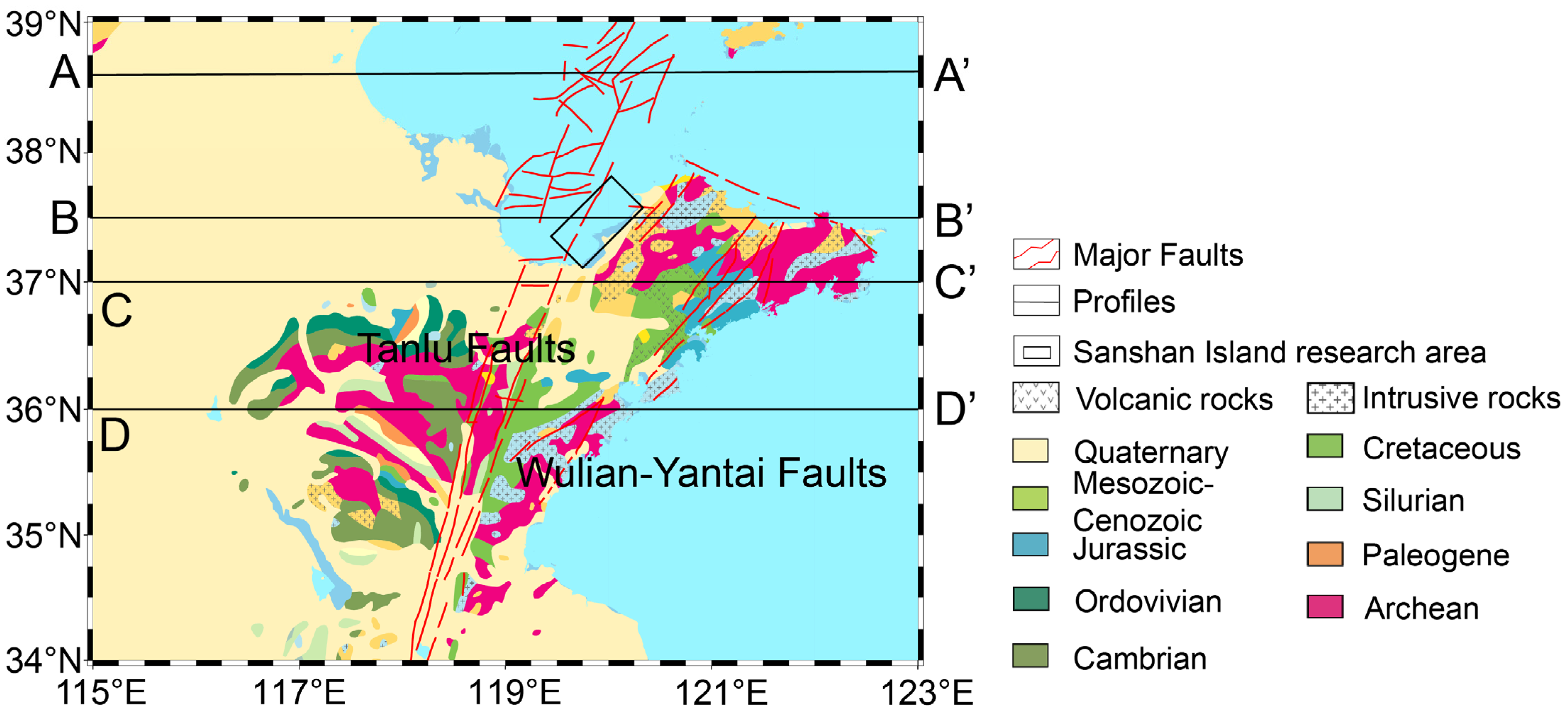
3.1. Geological Background
3.2. Data
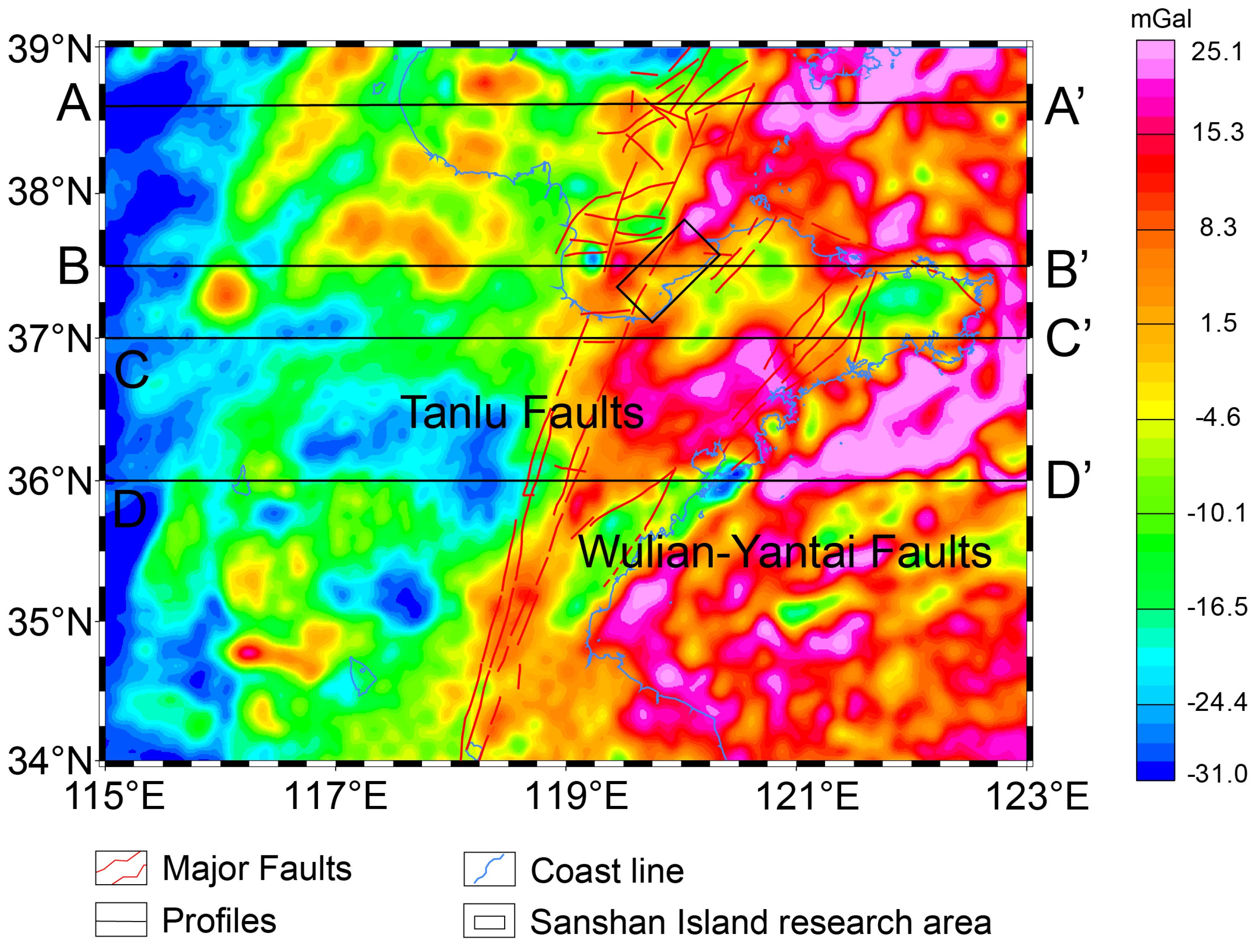
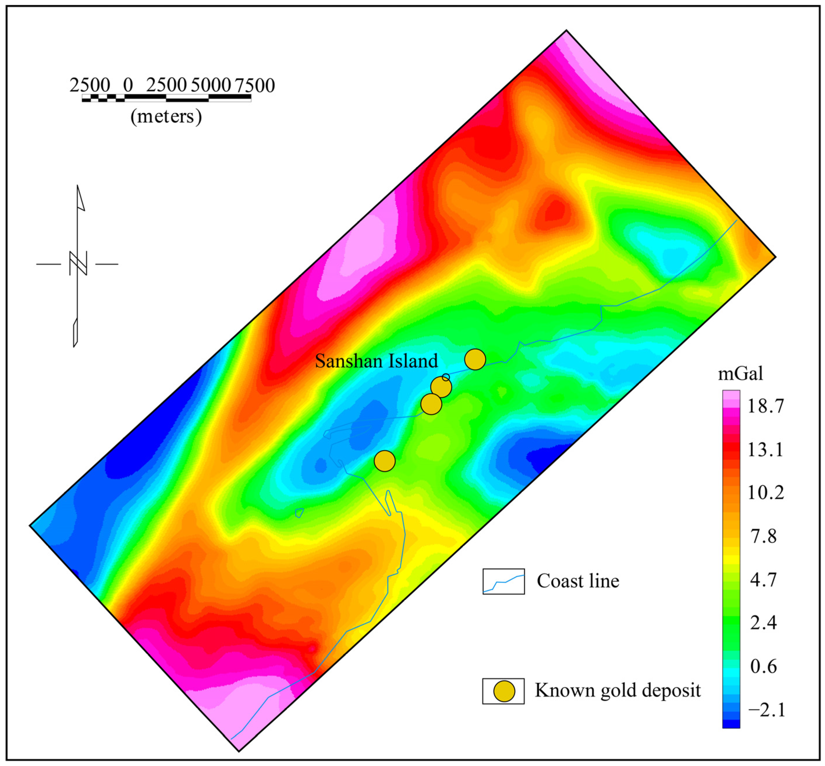
3.2.1. Gravity Data
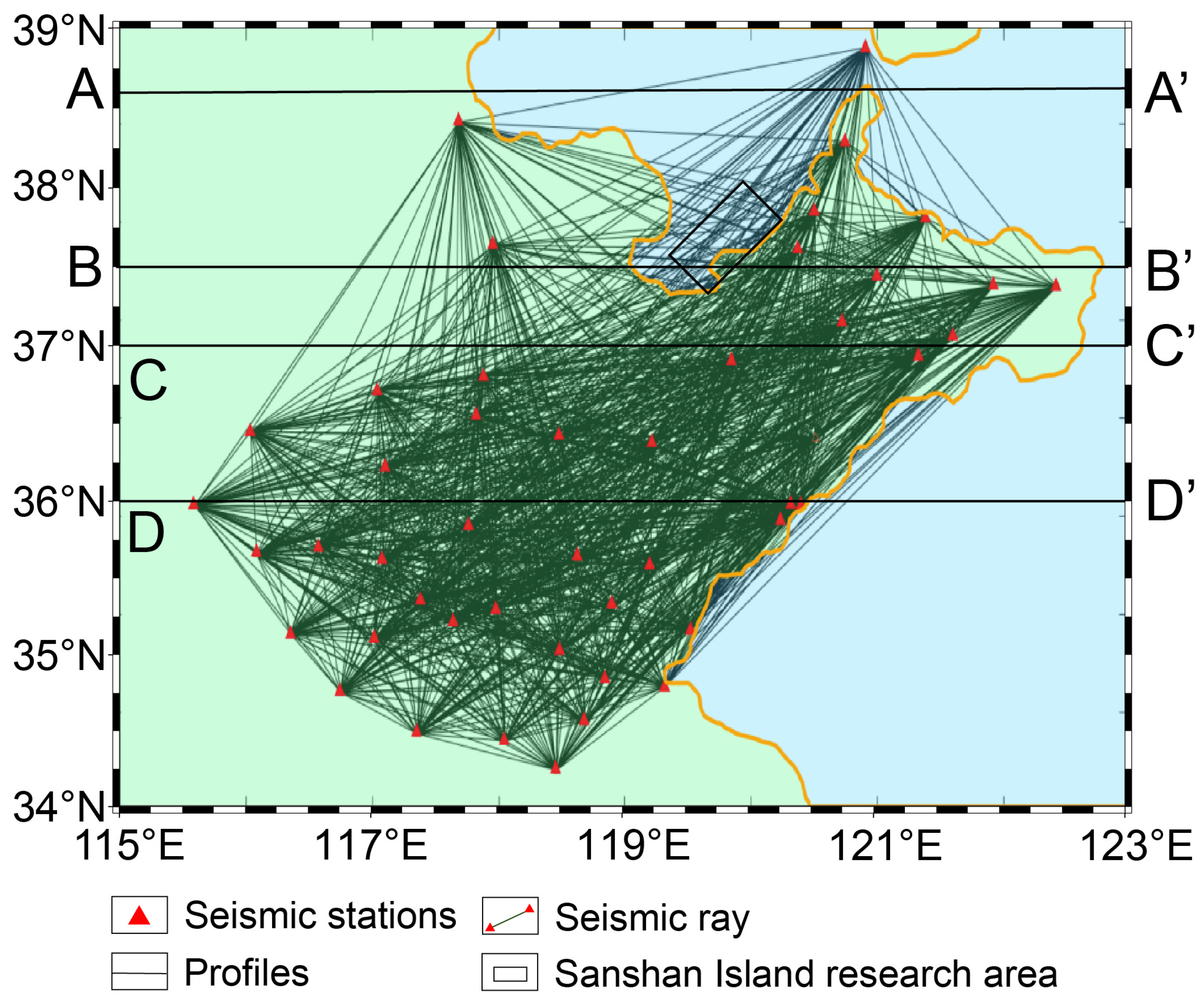
3.2.2. Seismic Data
3.3. Results
3.4. Further Inversion
4. Discussion
5. Conclusions
Author Contributions
Funding
Data Availability Statement
Conflicts of Interest
References
- Shapiro, N.M.; Campillo, M.; Stehly, L.; Ritzwoller, M.H. High-resolution surface-wave tomography from ambient seismic noise. Science 2005, 307, 1615–1618. [Google Scholar] [CrossRef] [PubMed]
- Yao, H.; van der Hilst, R.D.; van der Hoop, M. Surface-wave array tomography in SE Tibet from ambient seismic noise and two-station analysis—I. Phase velocity maps. Geophys. J. Int. 2006, 166, 271–288. [Google Scholar] [CrossRef]
- Yang, Y. Rayleigh wave phase velocity maps of Tibet and the surrounding regions from ambient seismic noise tomography. Geochem. Geophys. Geosyst. 2010, 11, Q08010. [Google Scholar] [CrossRef]
- Yang, Y.; Ritzwoller, M.H.; Zheng, Y.; Shen, W.; Levshin, A.L.; Xie, Z. A synoptic view of the distribution and connectivity of the mid-crustal low velocity zone beneath Tibet. J. Geophys. Res. Solid Earth 2012, 117. [Google Scholar] [CrossRef]
- Maceira, M.; Ammon, C. Joint inversion of surface wave velocity and gravity observations and its application to Central Asian basins shear velocity structure. Seismol. Res. Lett. 2006, 77, 297–302. [Google Scholar] [CrossRef]
- Guo, Z.; Chen, Y.S.; Yin, W.W. Three-dimensional crustal model of Shanxi graben from 3D joint inversion of ambient noise surface wave and Bouguer gravity anomalies. Chin. J. Geophys. 2015, 58, 821–831. [Google Scholar]
- Roecker, S.; Ebinger, C.; Tiberi, C.; Mulibo, G.; Ferdinand-Wambura, R.; Mtelela, K.; Kianji, G.; Muzuka, A.; Gautier, S.; Albaric, J.; et al. Subsurface images of the Eastern Rift, Africa, from the joint inversion of body waves, surface waves and gravity: Investigating the role of fluids in early-stage continental rifting. Geophys. J. Int. 2017, 210, 931–950. [Google Scholar] [CrossRef]
- Du, N.; Li, Z.; Hao, T.; Xia, X.; Shi, Y.; Xu, Y. Joint tomographic inversion of crustal structure beneath the eastern Tibetan Plateau with ambient noise and gravity data. Geophys. J. Int. 2021, 227, 1961–1979. [Google Scholar] [CrossRef]
- Asgharzadeh, M.F.; Von Frese, R.R.B.; Kim, H.R.; Leftwich, T.E.; Kim, J.W. Spherical prism gravity effects by Gauss-Legendre quadrature integration. Geophys. J. Int. 2007, 169, 1–11. [Google Scholar] [CrossRef]
- Liang, Q.; Chen, C.; Li, Y.G. 3-D inversion of gravity data in spherical coordinates with application to the GRAIL data. J. Geophys. Res. Planets 2014, 119, 1359–1373. [Google Scholar] [CrossRef]
- Uieda, L.; Barbosa, V.C.F.; Braitenberg, C. Tesseroids: Forward-modeling gravitational fields in spherical coordinates. Geophysics 2016, 81, F41–F48. [Google Scholar] [CrossRef]
- Uieda, L.; Barbosa, V.C.F. Fast nonlinear gravity inversion in spherical coordinates with application to the South American Moho. Geophys. J. Int. 2017, 208, 162–176. [Google Scholar] [CrossRef]
- Zhang, Y.; Wu, Y.; Yan, J.; Wang, H.; Rodrigues, J.A.; Qiu, Y. 3D inversion of full gravity gradient tensor data in spherical coordinate system using local north-oriented frame. Earth Planets Space 2018, 70, 58. [Google Scholar] [CrossRef]
- Wang, N.; Ma, G.; Li, L.; Wang, T.; Li, D. A density-weighted and cross-gradient constrained joint inversion method of gravity and vertical gravity gradient data in spherical coordinates and its application to lunar data. IEEE Trans. Geosci. Remote Sens. 2022, 60, 4511211. [Google Scholar] [CrossRef]
- Bijwaard, H.; Spakman, W. Fast kinematic ray tracing of first-and later-arriving global seismic phases. Geophys. J. Int. 1999, 139, 359–369. [Google Scholar] [CrossRef]
- Chuntao, L. The methods and applications of 3D ray tracing on spherical coordinate. Comput. Technol. Geophys. Geochem. Explor. 2001, 23, 199–205. [Google Scholar]
- De Kool, M.; Rawlinson, N.; Sambridge, M. A practical grid-based method for tracking multiple refraction and reflection phases in three-dimensional heterogeneous media. Geophys. J. Int. 2006, 167, 253–270. [Google Scholar] [CrossRef]
- Hu, G.; Bai, C.; Greenhalgh, S. Fast and accurate global multiphase arrival tracking; the irregular shortest-path method in a 3-D spherical Earth model. Geophys. J. Int. 2013, 194, 1878–1892. [Google Scholar]
- Huang, G.J.; Bai, C.Y. Simultaneous inversion of three model parameters with multiple classes of arrival times. Acta Geophys. Sin. 2013, 56, 4215–4225. [Google Scholar]
- Roussel, C.; Verdun, J.; Cali, J.; Masson, F. Complete gravity field of an ellipsoidal prism by Gauss-Legendre quadrature. Geophys. J. Int. 2015, 203, 2220–2236. [Google Scholar] [CrossRef]
- Bullen, K.E. An Introduction to the Theory of Seismology, 3rd ed.; Cambridge University Press: Cambridge, UK, 1963. [Google Scholar]
- Dziewonski, A.M.; Gilbert, F. The effect of small, aspherical perturbations on travel times and a re-examination of the corrections for ellipticity. Geophys. J. R. Astron. Soc. 1976, 44, 7–17. [Google Scholar] [CrossRef]
- Li, X.W.; Bai, C.Y. Multiple-phase seismic ray tracing in ellipsoidal coordinates. Chin. J. Geophys. 2017, 60, 3368–3377. [Google Scholar]
- Tang, X.P.; Bai, C.Y. Multiple ray tracing within 3-D layered media with the shortest path method. Acta Geophys. Sin. 2009, 52, 2635–2643. [Google Scholar]
- Bai, C.Y.; Tang, X.P.; Zhao, R. 2-D/3-D multiply transmitted, converted and reflected arrivals in complex layered media with the modified shortest path method. Geophys. J. Int. 2009, 179, 201–214. [Google Scholar] [CrossRef]
- Groves, D.I.; Liang, Z.; Santosh, M. Subduction, mantle metasomatism, and gold: A dynamic and genetic conjunction. Geol. Soc. Am. Bull. 2020, 132, 1419–1426. [Google Scholar] [CrossRef]
- Deng, J.; Yang, L.; Song, Z.; Wang, J.; Wang, Q.; Xu, H.; Liu, X. A metallogenic model of gold deposits of the Jiaodong granite-greenstone belt. Acta Geol. Sin. 2003, 77, 537–546. [Google Scholar]
- Jun, D.; Kunfeng, Q.; Qingfei, W.; Richard, G.; Liqiang, Y.; Jianwei, Z.; Jianzhen, G.; Yao, M. In situ dating of hydrothermal monazite and implications for the geodynamic controls on ore formation in the Jiaodong gold province, eastern China. Econ. Geol. 2020, 115, 671–685. [Google Scholar]
- Deng, J.; Wang, Q.; Santosh, M.; Liu, X.; Liang, Y.; Yang, L.; Zhao, R.; Yang, L. Remobilization of metasomatized mantle lithosphere: A new model for the Jiaodong gold province, eastern China. Miner. Depos. 2020, 55, 257–274. [Google Scholar] [CrossRef]
- Zhai, M.G.; Fan, H.R.; Yang, J.H.; Miao, L.C. Intracontinental Metallogenesis of Non-Orogenic Gold Deposits: The Jiaodong-Type Gold Deposits. Earth Sci. Front. 2004, 11, 14–30. [Google Scholar]
- Liqiang, Y.; Jun, D.; Zhongliang, W.; Liang, Z.; Linnan, G.; Mingchun, S.; Xiaoli, Z. Mesozoic gold metallogenic system of the Jiaodong gold province, eastern China. Acta Petrol. Sin. 2014, 30, 2447–2467. [Google Scholar]
- Mingchun, S.; Sanzhong, L.; Santosh, M.; Xuefei, L.; Yayun, L.; Liqiang, Y.; Rui, Z.; Lin, Y. Types, characteristics and metallogenesis of gold deposits in the Jiaodong Peninsula, eastern North China Craton. Ore Geol. Rev. 2015, 65, 612–625. [Google Scholar]
- Rixiang, Z.; Hongrui, F.; Jianwei, L.; Qingren, M.; Shengrong, L.; Qingdong, Z. Decratonic gold deposits. Sci. China Earth Sci. 2015, 58, 1523–1537. [Google Scholar]
- Wen, B.J.; Fan, H.R.; Hu, F.F.; Liu, X.; Yang, K.F.; Sun, Z.F. Fluid evolution and ore genesis of the giant Sanshandao gold deposit, Jiaodong gold province, China; constrains from geology, fluid inclusions and H–O–S–He–Ar isotopic compositions. J. Geochem. Explor. 2016, 171, 96–112. [Google Scholar] [CrossRef]
- Fan, H.; Lan, T.; Li, X.; Santosh, M.; Yang, K.; Hu, F.; Feng, K.; Hu, H.; Pemh, H.; Zhang, Y. Conditions and processes leading to large-scale gold deposition in the Jiaodong province, eastern China. Sci. China Earth Sci. 2021, 64, 1504–1523. [Google Scholar] [CrossRef]
- Goldfarb, R.J.; Santosh, M. The dilemma of the Jiaodong gold deposits: Are they unique? Geosci. Front. 2014, 5, 139–153. [Google Scholar] [CrossRef]
- Zhu, R.; Sun, W. The big mantle wedge and decratonic gold deposits. Sci. China Earth Sci. 2021, 64, 1451–1462. [Google Scholar] [CrossRef]
- Jun, D.; Xuefei, L.; Qingfei, W.; Ruiguang, P. Origin of the Jiaodong-type Xinli gold deposit, Jiaodong Peninsula, China; constraints from fluid inclusion and C–D–O–S–Sr isotope compositions. Ore Geol. Rev. 2015, 65, 674–686. [Google Scholar]
- Kunfeng, Q.; Jun, D.; Laflamme, C.; Long, Z.; Wan, R.; Moynier, F.; Yu, H.; Zhang, J.; Ding, Z.; Goldfarb, R. Giant Mesozoic gold ores derived from subducted oceanic slab and overlying sediments. Geochim. Cosmochim. Acta 2023, 343, 133–141. [Google Scholar]
- Chen, Y.M.; Zeng, Q.D.; Sun, Z.F.; Wang, Z.K.; Fan, H.R.; Xiao, F.L.; Chu, S.X. Study on geochemical background field of the gold deposits in Jiaodong, China. Gold Sci. Technol. 2019, 27, 791–801. [Google Scholar]
- Xiong, L.; Zhao, X.; Wei, J.; Jia, X.; Fang, L.; Li, Z. Linking Mesozoic lode gold deposits to metal-fertilized lower continental crust in the North China Craton: Evidence from Pb isotope systematics. Chem. Geol. 2020, 533, 119440. [Google Scholar] [CrossRef]
- Wang, Z.; Chen, H.; Zhang, K.; Guo, X.; Li, Y.; Yang, J.; Wang, F.; Becker, H.; Foley, S.; Wang, C.Y. Metasomatized lithospheric mantle for Mesozoic giant gold deposits in the North China Craton. Geology 2020, 48, 169–173. [Google Scholar] [CrossRef]
- Xiang, W.; Wang, Z.; Chen, H.; Zhang, K.; Wu, C.Y.; Meng, L.; Chen, Y.; Foley, S.; Hou, Z. Gold endowment of the metasomatized lithospheric mantle for giant gold deposits: Insights from lamprophyre dikes. Geochim. Cosmochim. Acta 2022, 316, 21–40. [Google Scholar]
- Xu, Z.; Wang, Z.; Guo, J.L.; Liu, H.; Guo, J.; Cheng, H.; Chen, K.; Wang, X.; Zong, K.; Zhu, Z.; et al. Chalcophile elements of the Early Cretaceous Guojialing granodiorites and mafic enclaves, eastern China, and implications for the formation of giant Jiaodong gold deposits. J. Asian Earth Sci. 2022, 238, 105374. [Google Scholar] [CrossRef]
- Deng, J.; Wang, Q.F.; Zhang, L.; Xue, S.C.; Liu, X.F.; Yang, L.; Yang, L.Q.; Qiu, K.F.; Liang, Y.Y. Genetic model of Jiaodong-type gold deposits. Sci. China Earth Sci. 2023, 53, 2323–2347. [Google Scholar]
- Zheng, Y.F.; Xiao, W.J.; Zhao, G. Introduction to tectonics of China. Gondwana Res. 2013, 23, 1189–1206. [Google Scholar] [CrossRef]
- Zheng, Y.F.; Xu, Z.; Zhao, Z.F.; Dai, L.Q. Mesozoic mafic magmatism in North China and craton thinning and destruction. Sci. China Earth Sci. 2018, 48, 379–414. [Google Scholar]
- Zheng, Y.; Chen, Y.; Chen, R.; Dai, L. Tectonic evolution of convergent plate margins and its geological effects. Sci. China Earth Sci. 2022, 65, 1247–1276. [Google Scholar] [CrossRef]
- Brocher, T.M. Empirical Relations between Elastic Wavespeeds and Density in the Earth’s Crust. Bull. Seismol. Soc. Am. 2005, 95, 2081–2092. [Google Scholar] [CrossRef]
- Portniaguine, O.; Zhdanov, M. 3-D magnetic inversion with data compression and image focusing. Geophysics 2002, 67, 1532–1541. [Google Scholar] [CrossRef]
- Utsugi, M. 3-D inversion of magnetic data based on the L1–L2 norm regularization. Earth Planets Space 2019, 73, 71. [Google Scholar] [CrossRef]
- Farquharson, C.G.; Oldenburg, D.W. Non-linear inversion using general measures of data misfit and model structure. Geophys. J. Int. 1998, 134, 213–227. [Google Scholar] [CrossRef]
- Zhdanov, M.S. Geophysical Inverse Theory and Regularization Problems; Elsevier: Amsterdam, The Netherlands, 2002. [Google Scholar]
- Laske, G.; Masters, G.; Ma, Z.; Pasyanos, M. Update on CRUST1.0—A 1-degree global model of Earth’s crust. Geophys. Res. Abstr. 2013, 15, 2658. [Google Scholar]
- Miller, H.G.; Singh, V. Potential field tilt: A new concept for location of potential field sources. J. Appl. Geophys. 1997, 32, 213–217. [Google Scholar] [CrossRef]
- Song, M.; Zhang, J.; Zhang, P.; Yang, L.; Liu, D.; Ding, Z.; Song, Y. Discovery and tectonic-magmatic background of a super-large gold deposit offshore of northern Sanshandao, Shandong Peninsula, China. Acta Geol. Sin. 2015, 89, 365–383. [Google Scholar]
- Chai, P.; Hou, Z.; Zhang, Z. Geology, fluid inclusion and stable isotope constraints on the fluid evolution and resource potential of the Xiadian gold deposit, Jiaodong Peninsula. Resour. Geol. 2017, 67, 341–359. [Google Scholar] [CrossRef]
- Yu, G.; Xu, T.; Liu, J.; Ai, Y. Late Mesozoic extensional structures and gold mineralization in Jiaodong Peninsula, eastern North China Craton: An inspiration from ambient noise tomography on data from a dense seismic array. Chin. J. Geophys. 2020, 63, 1878–1893. [Google Scholar]
- Deng, J.; Wang, Q.; Liu, X.; Zhang, L.; Yang, L.; Yang, L.; Qiu, K.; Guo, L.; Liang, Y.; Ma, Y. The formation of the Jiaodong gold province. Acta Geol. Sin. Engl. Ed. 2022, 96, 1801–1820. [Google Scholar] [CrossRef]


Disclaimer/Publisher’s Note: The statements, opinions and data contained in all publications are solely those of the individual author(s) and contributor(s) and not of MDPI and/or the editor(s). MDPI and/or the editor(s) disclaim responsibility for any injury to people or property resulting from any ideas, methods, instructions or products referred to in the content. |
© 2025 by the authors. Licensee MDPI, Basel, Switzerland. This article is an open access article distributed under the terms and conditions of the Creative Commons Attribution (CC BY) license (https://creativecommons.org/licenses/by/4.0/).
Share and Cite
Ma, G.; Jiang, Z.; Cao, R.; Yan, J.; Liu, H.; Meng, Q.; Wang, N.; Li, L. The Joint Inversion of Seismic Ambient Noise and Gravity Data in an Ellipsoidal Coordinate System: A Case Study of Gold Deposits in the Jiaodong Peninsula. Minerals 2025, 15, 488. https://doi.org/10.3390/min15050488
Ma G, Jiang Z, Cao R, Yan J, Liu H, Meng Q, Wang N, Li L. The Joint Inversion of Seismic Ambient Noise and Gravity Data in an Ellipsoidal Coordinate System: A Case Study of Gold Deposits in the Jiaodong Peninsula. Minerals. 2025; 15(5):488. https://doi.org/10.3390/min15050488
Chicago/Turabian StyleMa, Guoqing, Zhexin Jiang, Rui Cao, Jiayong Yan, Hongbo Liu, Qingfa Meng, Nan Wang, and Lili Li. 2025. "The Joint Inversion of Seismic Ambient Noise and Gravity Data in an Ellipsoidal Coordinate System: A Case Study of Gold Deposits in the Jiaodong Peninsula" Minerals 15, no. 5: 488. https://doi.org/10.3390/min15050488
APA StyleMa, G., Jiang, Z., Cao, R., Yan, J., Liu, H., Meng, Q., Wang, N., & Li, L. (2025). The Joint Inversion of Seismic Ambient Noise and Gravity Data in an Ellipsoidal Coordinate System: A Case Study of Gold Deposits in the Jiaodong Peninsula. Minerals, 15(5), 488. https://doi.org/10.3390/min15050488