Article

Antimony Ore Identification Method for Small Sample X-Ray Images with Random Distribution

1
State Key Laboratory of Coking Coal Resources Green Exploitation, China University of Mining and Technology, Xuzhou 221116, China
2
School of Information and Control Engineering, China University of Mining and Technology, Xuzhou 221116, China
3
Artificial Intelligence Research Institute, China University of Mining and Technology, Xuzhou 221116, China
*
Author to whom correspondence should be addressed.
Minerals 2025, 15(5), 483; https://doi.org/10.3390/min15050483
Submission received: 1 April 2025 / Revised: 28 April 2025 / Accepted: 2 May 2025 / Published: 5 May 2025
(This article belongs to the Special Issue Recent Advances in Ore Comminution)

Abstract

:
The performance of image processing is crucial for accurately sorting antimony ore, yet several challenges persist. Existing image segmentation methods struggle with X-ray ore images that contain high noise and interference. Additionally, traditional classification methods primarily utilize single physical properties, such as the R-value, leading to low accuracy. To address segmentation issues, this paper proposes an improved method based on concave detection. This involves obtaining a binary image of antimony ore through adaptive threshold segmentation, extracting the ore contour, and detecting concave points using advanced techniques. The influence of interfering concave points is minimized with the three-wire method, while noise points are reduced through morphological operations based on area calculations. This results in accurate segmentation of the adherent antimony ore. For classification, this paper introduces a training method that combines transfer learning with shallow partial initialization. Transfer learning is employed to mitigate the challenges of limited antimony ore datasets when using deep learning models. The pre-trained model is then partially re-initialized according to a tailored strategy. Finally, fine-tuning is performed on the antimony ore dataset to achieve optimal results. Experimental results show that the antimony ore segmentation method proposed in this paper achieves accurate segmentation (96.27% correct segmentation rate). The antimony ore classification model training method proposed in this paper can effectively release some redundant parameters of the pre-training model, and has better classification performance on the target dataset (86.76% accuracy). Both methods are superior to traditional methods.

1. Introduction

In the production process of ores, sorting is an indispensable link, and the efficacy of ore separation ultimately dictates whether the raw ore can be fully exploited [1]. In recent years, the dual-energy X-ray sorting methods have received increasing attention [2,3]. Most research has focused on sorting based on the physical characteristics of the ore itself [4]. However, there is little research on the segmentation of adherent antimony ores, which is essential in the ore sorting process. On the other hand, traditional mechanism-based classification methods represented by the R-value only use the physical properties of the ore as a single feature, and are easily affected by thickness effects, beam hardening effects, and afterglow effects, resulting in low classification accuracy.
In the realm of image segmentation, segmentation techniques leveraging concave point detection prove highly effective when it comes to segmenting circular attached objects [5,6,7,8]. This method primarily utilizes the prior knowledge that concave points will inevitably appear at the adhesion points of round-like objects to segment the adherent images [9,10,11,12,13,14]. For instance, Yao et al. [15] employed a concavity detection algorithm for segmenting rice, whereas Song et al. [16] introduced a technique that integrates concavity detection with the watershed method for segmenting adherent cells. The concave point detection-based segmentation method is characterized by its speed, making it suitable for real-time tasks, and it can achieve good results on smooth-surfaced objects like cells. Although antimony ore is also a round-like object, its physical properties result in many small interfering concave points on its surface. Directly using concave point detection will detect many small concave points, which, if not processed, will lead to significant over-segmentation.
In the field of image classification, convolutional neural networks (U-Net, VGG, ResNet) are widely used as important tools for image classification. They can effectively extract and utilize the hidden features in the target dataset by automatically executing feature extraction and self-learning, thereby reducing the influence of interference factors [17,18]. However, deep learning methods have two limitations. First, the training of deep learning models for ore classification methods relies on a large amount of data, but due to the different types of ores and some external factors, it is difficult to obtain image data from antimony ore. Second, deep learning models suffer from problems such as long training times, numerous model parameters, and difficulty in optimization [19]. Transfer learning can compensate for the above issues of insufficient antimony ore image data and slow model convergence on the target dataset. Generally, pre-trained models obtained through network-based deep transfer learning [20,21,22] have good feature extraction capabilities, which can be effectively applied to downstream tasks. However, during the transfer process, differences in data distribution may arise between the source domain and the target domain. This implies that pre-trained models, which have been trained on the source dataset, may not fully capture all of the features of the target dataset, and in extreme cases, it may even lead to negative transfer.
Pruning is a commonly used deep-learning model compression method. According to the specific methods used during the pruning process, pruning can be divided into importance-based pruning, reconstruction-based pruning, loss-gradient-change-based pruning, and similarity-based pruning. This paper focuses on importance-based pruning and similarity-based pruning. LI H [23] performed pruning based on the importance of convolutional kernels in the convolutional layer, calculating the absolute value of each kernel’s weight as the evaluation criterion and pruning several convolutional kernels with smaller absolute weight values, then retraining to restore network accuracy, achieving a good compression ratio. Liu Z [24] evaluated the importance of feature map channels by adding a scaling factor in the batch normalization layer and removing channels with higher sparsity. LIN M B et al. [25] believed that the rank of a feature map describes the independence of each vector of the feature and the richness of the feature information. The larger the rank, the stronger the independence of each vector, and the richer the feature information. They pruned the parameters of the convolutional layer based on the rank of the feature map after the convolution. Importance-based pruning focuses on the importance of convolutional kernels and feature maps for the entire task. In contrast, similarity-based pruning focuses on the similarity of convolutional kernels and feature maps within the same layer. HE Y [26] proposed a pruning criterion based on the geometric median of filters, selecting and pruning the filters with the smallest Euclidean distance sum to other filters in the same layer, thus removing redundant filters. In the existing literature, researchers pay more attention to the pruning method of a single criterion. Although some results have been achieved, there are few methods that integrate multiple criteria, especially in dynamically adjusting pruning strategies.
To solve the problems mentioned above, the main contributions of this paper are as follows: To address the existing problems in antimony ore image segmentation, this paper proposes a segmentation method for adherent antimony ore based on concave point detection. This method includes three parts: an adaptive threshold segmentation and image binarization module, a contour extraction module using Suzuki’s algorithm [27], a concave point detection module based on vector angle, and a concave point matching module based on auxiliary lines of concave points [28]. In order to solve the problems of insufficient data and long model training in the current ore image classification method, a model training approach that integrates shallow initialization of the model’s early layers with transfer learning has been introduced.

2. Materials and Methods
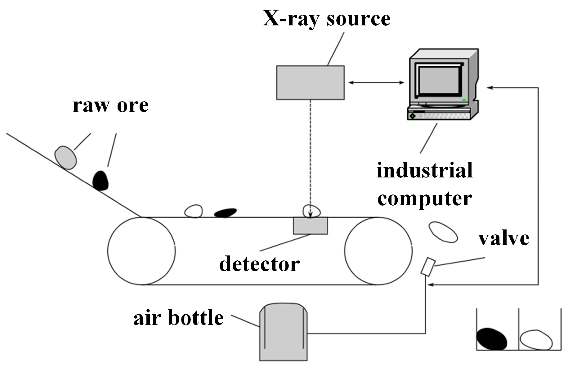
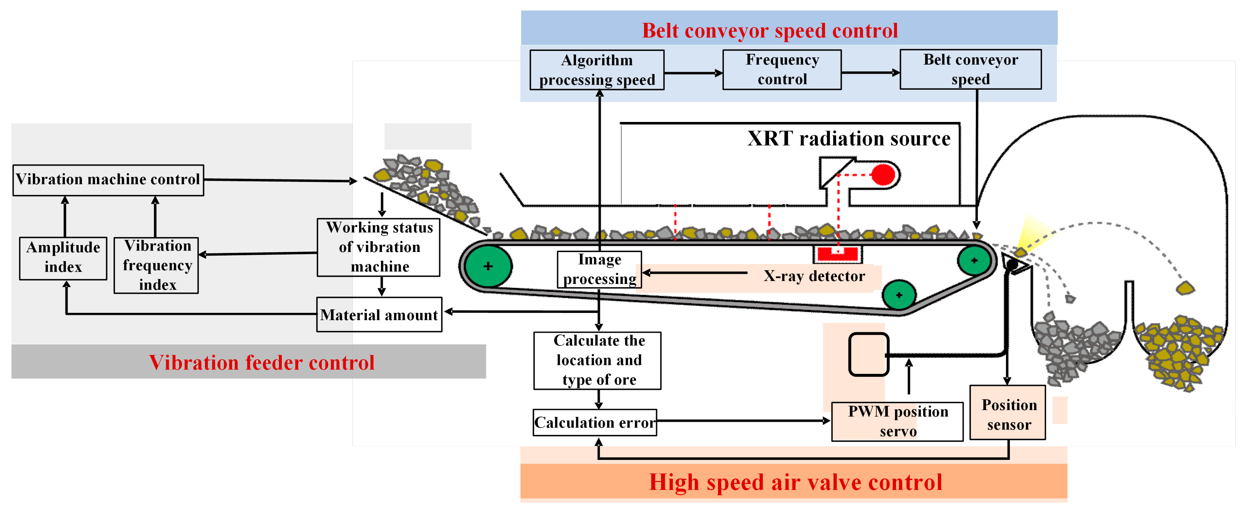
2.1. Materials

In this study, antimony ore was used for experimental verification. Antimony ore samples were collected from industrial partners in Shenyang Mineral Processing Zone, Liaoning, China Province, which is famous for its polymetallic deposits. In order to ensure the effectiveness of the experiment, a standardized preparation scheme was implemented, including jaw crushing (particle size < 10 mm) and rotary splitting, which realized the mineralogical uniformity, which is very important for the consistency of X-ray imaging. According to the economic feasibility and considering the process integrity, the samples are divided into three different categories: (1) concentrate (>25% antimony content), which represents economically feasible ore; (2) medium-grade ore (0.5%–5% antimony), which is a secondary economic material that needs mineral processing; and (3) tailings (<0.05% antimony), which represent the treatment waste stream.
A schematic diagram of a typical X-ray-based antimony ore sorting device is shown in Figure 1. The sorting process is as follows: The original antimony ore is crushed into small stones of uniform size, and then transported by conveyor belt to the pseudo dual energy X-ray identification device. The computer uses high- and low-energy images provided by the X-rays to determine the grade of the antimony ore and transmits its coordinates to an air valve. The air valve adjusts the air pressure based on these coordinates to blow the antimony ore into different sorting bins. In this process, the image processing algorithm’s ability to accurately segment the position of the antimony ore from the X-ray images and correctly classify the ore is essential for ensuring effective sorting.

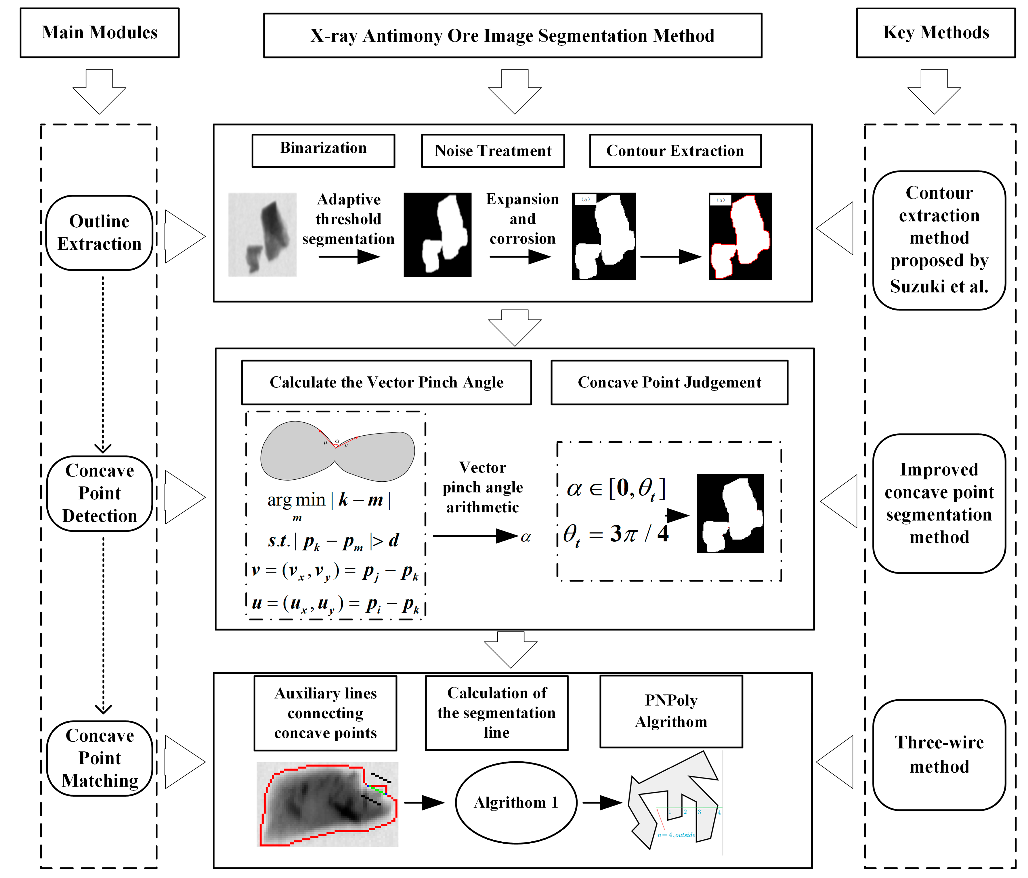
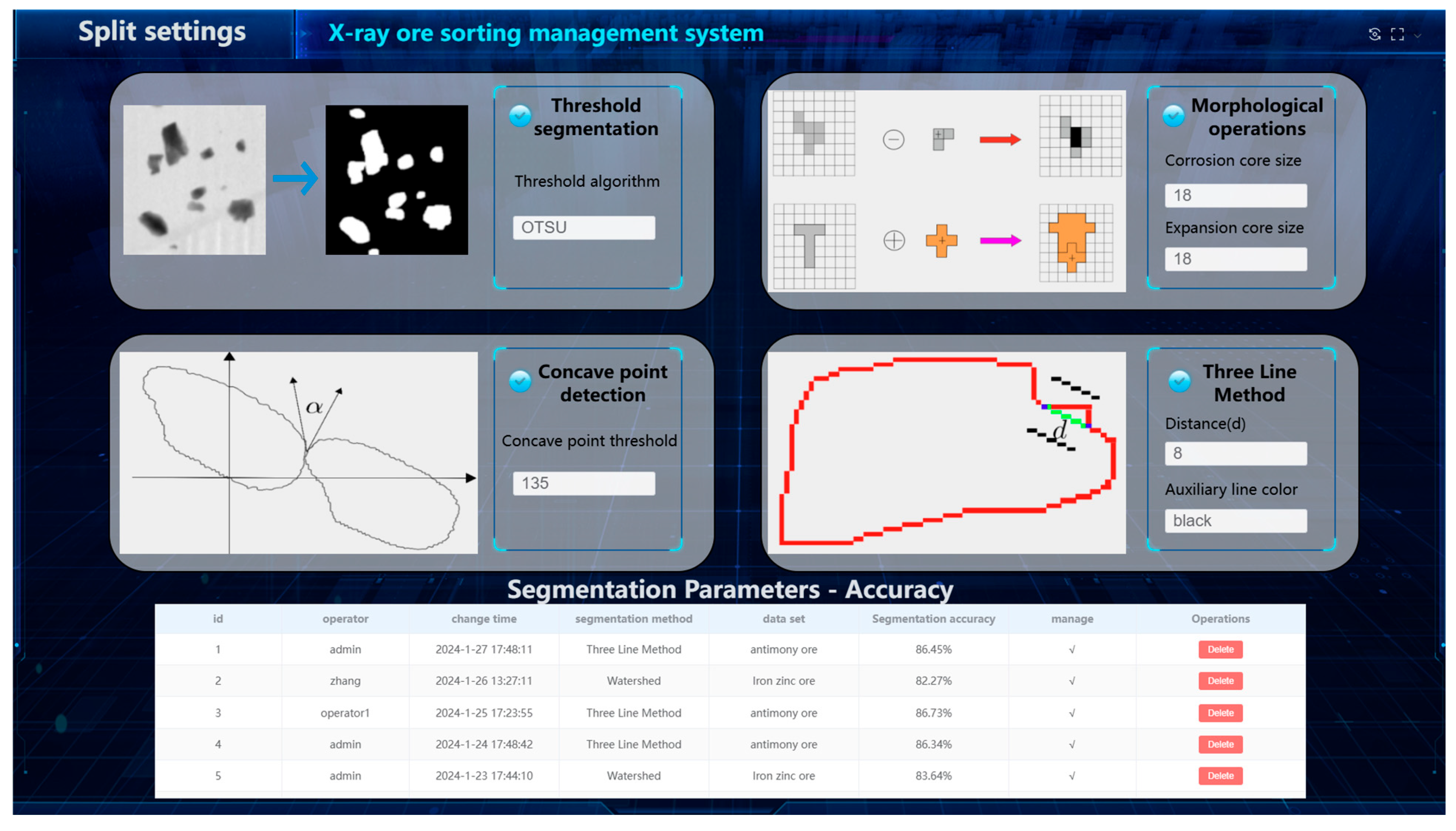
2.2. Design of X-Ray Antimony Ore Image Segmentation Method

Before achieving model classification, it is necessary to ensure that the adherent antimony ores in the collected image data are correctly segmented. This paper employs an X-ray-based antimony ore image segmentation method, which includes a contour extraction module, a concave point detection module, and a concave point matching module. The specific process is shown in Figure 2. The contour extraction module primarily involves image binarization, noise processing, and contour extraction. The concave point detection module mainly determines whether a contour point is a concave point by calculating the concavity of the contour points using the vector method. The concave point matching module is the main contribution of this section. It reduces the probability of over-segmentation by drawing auxiliary lines connecting concave points and determining the relative positions of these auxiliary lines and the antimony ore contours, thereby avoiding the interference of ore boundaries and the influence of concave points on matching.
In the contour extraction module, adaptive threshold segmentation is first used to binarize the image to segmentation-adherent images and to perform an initial segmentation of adherent images. To remove noise points in the antimony ore images, morphological operations such as dilation and erosion are used sequentially to eliminate noise points inside and outside the antimony ore. Finally, the method proposed by Suzuki et al. is used to identify the contour from the denoised binary image [27].
In the concave point detection module, the concavity of contour points is calculated using the vector method to the x-axis θ ( u x , u y ) and θ ( v x , v y ) is computed, and the difference between these results gives the angular difference θ 1 . The angle derived from the function in Equation (1), θ ( x , y ) is measured from the positive direction of the x-axis, with the angle range [ 0 , 2 π ] from 0 ° to counterclockwise, ending at 360 ° .
θ ( x , y ) = arctan ( y x ) x > 0 , y 0 arctan ( y x ) + π x < 0 arctan ( y x ) + 2 π y < 0 , x > 0 π 2 x = 0 , y > 0 3 π 2 x = 0 , y < 0
due to [ 0 , 2 π ] , the results need to be processed using Equation (2) to obtain the actual angle value α .
α = θ 1 + 2 π θ 1 ( 2 π , π ) θ 1 θ 1 [ π , π ] θ 1 2 π θ 1 ( π , 2 π )
We can intuitively determine the convexity and concavity of points on the contour, as well as the degree of concavity and convexity, from the value of α . It is stipulated that only when α [ 0 , θ t ] is considered a concave point. After repeated experiments, we can achieve a good concave point detection effect for our specific antimony ore samples, so this paper chooses θ t = 3 π / 4 as the threshold, and the selection of the threshold will have different effects for different samples.
This part’s main contribution is the concave matching module. It mainly constructs auxiliary lines connecting concave points to determine the distance between the auxiliary lines and the antimony ore contour, avoiding the influence of boundary interference on concave point matching, thus reducing the probability of over splitting. The auxiliary lines of concave point connections are actually parallel line segments to the concave point connections, with the same length as the concave point connections. Therefore, we only need to calculate the concave point coordinates and the coordinates of the end points of the auxiliary lines Δ x and Δ y based on the slope of the concave point connections d and their distance d from the auxiliary lines to ultimately obtain the auxiliary lines. Given the end point coordinates of the concave point connections ( r 0 , c 0 ) , ( r 1 , c 1 ) , we first calculate their slope k using Equation (3).
k = c 1 c 0 r 1 r 0
The absolute value of the difference in distance between the coordinates of the concave point and the coordinates of the endpoints of the auxiliary line can be obtained from the slope and the distance.
Δ x = k d 1 + k 2
Δ y = Δ x k
Translate the endpoint coordinates of the concave point ( r 0 , c 0 ) and ( r 1 , c 1 ) by Δ x and Δ y in the direction of the horizontal and vertical axes to get the endpoint coordinates of the auxiliary lines P 0 , P 1 , N 0 , N 1 on both sides of the concave point.
P 0 = ( r 0 + Δ x , c 0 + Δ y )
P 1 = ( r 1 + Δ x , c 1 + Δ y )
N 0 = ( r 0 Δ x , c 0 Δ y )
N 1 = ( r 1 Δ x , c 1 Δ y )
Connect the endpoints of the auxiliary line P 0 and P 1 to obtain the auxiliary line segment L P ; similarly, connect N 0 and N 1 to obtain the auxiliary line segment L N . By using the above method for each candidate segmentation line, the true segmentation line of adherent antimony ore can be found from the candidate segmentation lines. The detailed description of Algorithm 1 is shown below:
Algorithm 1: Calculate candidate segmentation lines.
Input: The set of concave points on the contour C, the contour.
Output: Collection of segmentation lines L l i s t .
Step 1. For the set of concave points C = { p 1 , p 2 , , p n } get the permutations { p 1 , p 2 } , { p 1 , p 3 } , { p i , p j } , …, { p n 1 , p n }
Step 2. Calculate the distance between elements D = { d 1 , 2 , d 1 , 3 , d i , j ,…, d n 1 , n } ,where d i , j = | p i p j |
Step 3. Find the smallest value d k , q in the set D
Step 4. Remove p k , t ,   p t , q in set D where t = 1 , 2 , , n
Step 5. Repeat steps 3–4, until there are fewer than 2 elements in C
Step 6. For all line L of the C L l i s t do
Plot its auxiliary line at distance d L s i b l i n g s ;
If L s i b l i n g s are all in contours then
Addition L to L l i s t .
End if
End for

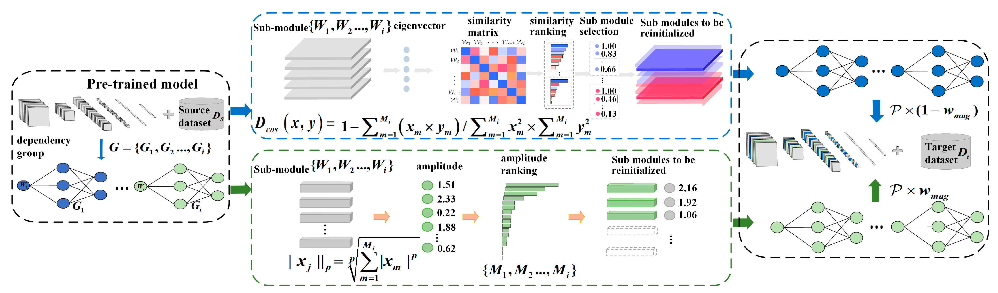
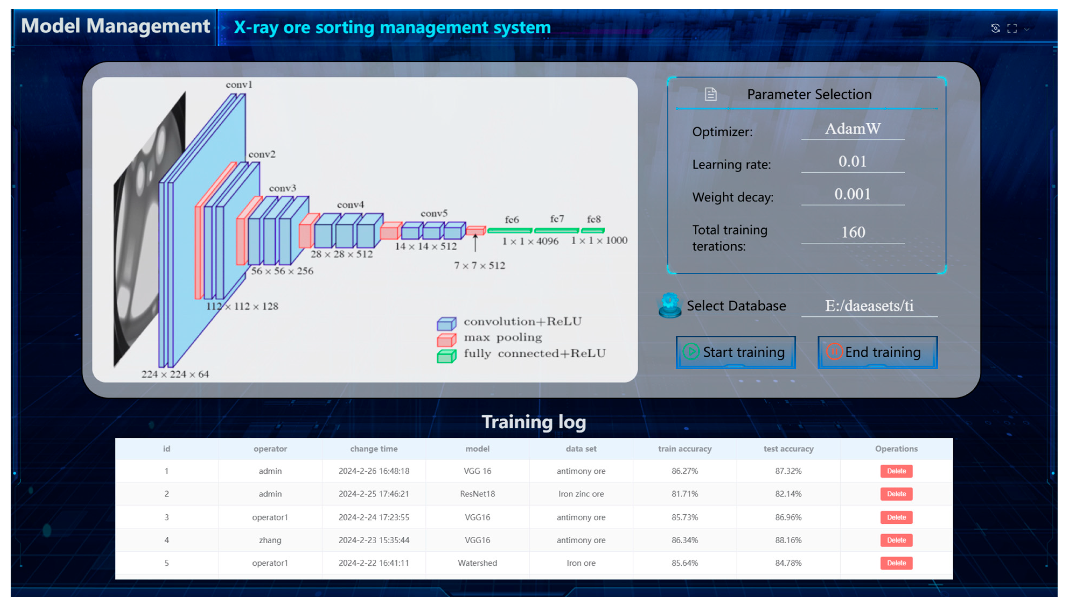
2.3. A Method for Ore Classification Incorporating Transfer Learning and Model Shallow Part Initialization

The schematic diagram of the proposed antimony ore classification model training method is shown in Figure 3. It mainly consists of the following steps: 1. Model pre-training. 2. Partial reinitialization of the pre-trained model. 3. Fine-tuning of the partially initialized model on the target dataset. First, the model needs to be pre-trained on a larger dataset. Next, following the method proposed in Ref. [29], the model’s sub-modules are divided into multiple dependency groups G according to their dependency relationships. These dependency groups are then ranked based on similarity and magnitude of importance evaluation criteria. The less important dependency groups undergo shallow partial reinitialization. In this process, a parameter is introduced to balance the importance and similarity indicators for the partial reinitialization parameter ratio.

2.3.1. Model Pre-Training

First, it is necessary to obtain a pre-trained model from a large dataset. Pre-trained models typically require a large amount of data to learn rich feature representations, and the size of the dataset directly affects the performance of the model. Additionally, the dataset should contain diverse samples so that the model can learn a wide range of features and patterns, which helps the model adapt better to the task of mineral classification. While meeting the requirements for dataset size and diversity, the higher the relevance of the dataset to the target task, the better the performance of the pre-trained model usually is.

2.3.2. Partial Reinitialization of the Pre-Trained Model

In this paper, we adopt the same notation as He et al. [26]. For a neural network with L layers, where N i and N i + 1 represent the number of input and output channels of the K × K th layer, respectively, the K × K convolution kernel of the 1 j N i + 1 th layer can be represented as F i , j N i × K × K . Thus, for the i th convolutional layer, the set of convolution kernels in the network can be represented as 1 j N i + 1 , and its weight values can be represented as W ( i ) N i + 1 × N i × K × K . For simplicity, this paper represents the weight values of the convolution kernel F i , j of the i th layer as a one-dimensional vector X N i + 1 × M i , which means that there are M convolution kernel vectors in the N i + 1 th convolutional layer, and each vector has a size of M i = N i × K × K .
To release more parameters in the shallow layers for learning features that better fit the target dataset, this paper needs to adopt a model pruning approach to find convolutional kernels that can be partially reinitialized. The goal of the algorithm is to iteratively select and partially reinitialize unimportant groups of convolutional kernels. This way, after partial reinitialization, the convolutional kernels that have not been reinitialized can still extract features from the source dataset as effectively as possible, minimizing the loss of accuracy in the partially reinitialized model. This paper uses amplitude and similarity measures, two widely used metrics, to assess the similarity of convolutional kernels.
In the field of model pruning, researchers have long discovered that parameters with smaller weights can be safely pruned without affecting the model’s performance, a principle that also applies to pruning convolutional kernels. Li et al. [23] demonstrated through extensive experiments that convolutional kernels with smaller norms have less impact on the model’s final classification results compared to kernels with larger norms, and thus can be removed. In this paper, we also use the norm of the convolutional kernels as a measure of their importance. M i , as mentioned above, is the vector size of the single-layer convolution kernel. If the convolution kernel of the X j layer is expressed as x 1 × M i , its p norm can be calculated by Equation (10).
| | x j | | p = m = 1 M i | x m | p p
While convolutional kernels with smaller amplitudes can be safely removed as redundant parameters, those with larger amplitudes may also be redundant. He et al. [26,27,28,30] proposed that similarity can also serve as an evaluation metric for the importance of convolutional kernels, in addition to amplitude. Since convolutional kernels with high similarity can extract similar image features, one of them can be safely removed without affecting the model’s performance. Therefore, this paper comprehensively uses both amplitude and similarity as evaluation metrics for the importance of convolutional kernels. Methods for calculating convolutional kernel similarity typically include Euclidean similarity and cosine similarity. This paper selects cosine similarity, as shown in Equation (11), as the evaluation metric.
D c o s x , y = 1 m = 1 M i x m × y m m = 1 M i x m 2 × m = 1 M i y m 2
D c o s x , y is the cosine distance measure, x and y are the two convolution kernel parameter vectors to be compared, and M i is the same as mentioned above.
In this paper, an iterative approach is used to prune convolutional kernels. During each iteration, after measuring the importance of convolutional kernels using Equation (10) or Equation (11), the algorithm selectively reinitializes the least important convolutional kernels in a structured manner. This means that the algorithm not only reinitializes the least important convolutional kernels, but also reinitializes a portion of the parameters corresponding to the subsequent connected convolutional kernels, resulting in a final actual reinitialization rate P r that is higher than the set value P .
To maximize the release of redundant parameters in the convolutional kernels using both amplitude and similarity as metrics for convolutional kernel similarity, this paper uses an initialization rate P to determine when to use amplitude or similarity indicators. The ultimate goal of partially reinitializing the convolutional kernels is to achieve a proportion of free parameters in the shallow layer L s h a l l o w that is greater than or equal to the given initialization rate P through iterative partial reinitialization. The formula for the initialization rate is shown in Equation (12).
P = 1 f f l o p ( W ) f f l o p ( W )
f f l o p ( W ) represents the number of parameters of the trimmed model, and f f l o p ( W ) represents the number of parameters of the pre-trained model.
In the initial stage, this paper uses an amplitude-based importance criterion for reinitialization. After a certain degree of reinitialization, it switches to a similarity-based criterion for partial initialization of the model. This method is chosen because after removing convolutional kernels with smaller amplitudes, those with larger amplitudes may be similar to each other. These similar convolutional kernels can be redundant, as they can be mutually replaceable in feature extraction and processing. Given a magnitude pruning ratio w m a g , approximately P × w m a g proportion of parameters are pruned using the amplitude-based criterion during the algorithm’s execution, while the remaining P × ( 1 w m a g ) are partially reinitialized using the similarity criterion. In this paper, w m a g is set to 0.5 to make both pruning criteria equally effective.
The detailed algorithm for pre-trained model reinitialization is shown in Algorithm 2. Given a pre-trained model M p , a pruning initialization rate P , and an amplitude pruning ratio w m a g , the algorithm iteratively selects unimportant convolutional kernels and obtains their corresponding dependent groups G . It then partially reinitializes all sub-modules in the dependent groups. After calculating the new reinitialization rate P , the algorithm compares P with the target initialization rate P . If it does not meet the criteria, the initialization operation continues until the initialized proportion P is greater than the target initialization rate P , resulting in the final partially initialized model.
Algorithm 2: Pre-trained model reinitialization
Input: Dataset D s , pre-trained model M p , given initialization rate W 1 , magnitude pruning ratio w m a g .
Output: Models after reinitialization M r .
Step 1. Initialization: W W , P 0 , List of trimmed parameters: P l i s t { }
Step 2. Find all submodules W i and their corresponding dependency groups in the shallow module G = { G 1 , G 2 , , G i }
Step 3. While P < P do
If  P P × w m a g  then
For  j in 1 , 2 , , i do
Calculate the magnitude of the convolutional kernel amplitude { M 1 , M 2 , , M i } for each sub-module in the model according to Equation (10) and get the smallest amplitude M m i n
End for
Else
For j in 1 , 2 , , i do
Calculate the similarity matrix S = s 11 s 12 s 1 n s 21 s 22 s 2 n s m 1 s m 2 s m n between the sub-modules according to Equation (11), where s i j denotes the similarity between the i th matrix and the j th matrix.
Sort the items in the similarity matrix in descending order: s 1 , s 2 , , s n .If s 1 = s x y is the maximum of these, then crop out M x and remove the M y , k term in the similarity matrix from the module to be cropped, where k { 1 , 2 , 3 , , n } and M t , y where t { 1 , 2 , , m } . Avoid that M y -related terms are also cropped out.Add M x and the corresponding parameter corresponding to it in the dependency group G to P l i s t .
End for
End if
End while

2.3.3. Reinitialize Model Training

After obtaining the reinitialized model M r with some of the shallow parameters released, the shallow parts of the parameters are assigned one by one to the completely reinitialized model M n to obtain the target model M n with the shallow partially initialized and the deep layer fully initialized, and then the model M n is trained on the target dataset D t to obtain the final fine-tuned model M d . It should be noted that in the traditional deep learning training framework, the model parameters are updated in terms of the complete convolutional layer weights W ( i ) . Therefore, in this paper, the extraction capability of the model obtained by training on the original dataset D s is maintained during the model training process by retaining the shallow part of the uncropped parameters before parameter updating of the model training and restoring the retained parameters after the training.

3. Results and Discussion

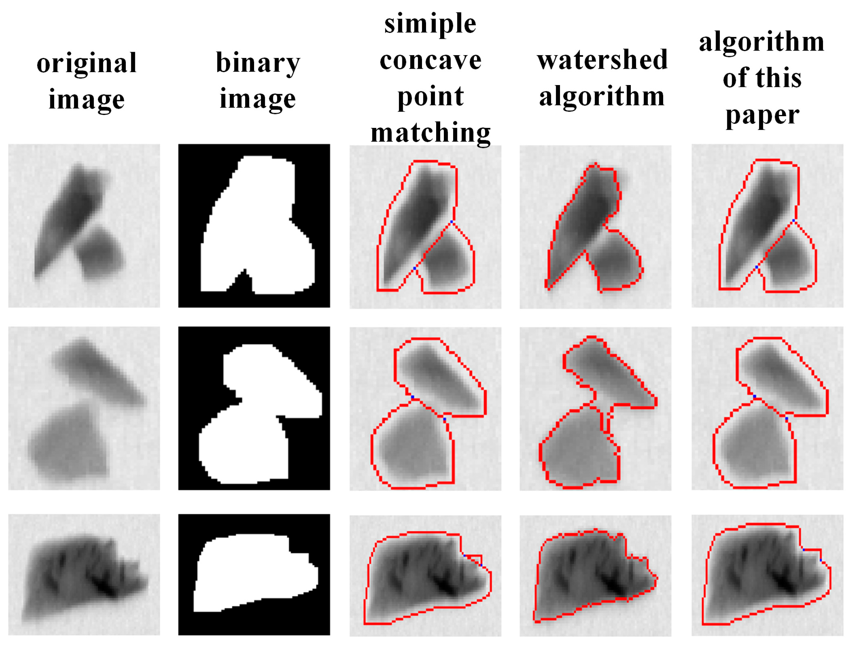
3.1. Experiments on an Improved Antimony Ore Segmentation Method Based on Concave Point Detection

All simulation experiments in this paper are run on a computer equipped with an Intel-i9-12900kx 24 CPU and a GeForce RTX3090 GPU. We verify the image segmentation algorithm using Python 3.8.8 and OpenCV 4.5.5. The PyTorch software 1.12.x library is used to verify the deep learning image classification algorithm.
In order to verify the effect of the algorithm in this paper, this paper selects antimony ore to carry out experiments, and the relevant parameters of the samples are shown in Table 1. This paper selects 119 single channel 512 × 5632 16-bit depth gray images.
In order to better illustrate the problem, this article compares concave point matching based on the trilinear method with simple concave point matching and the watershed algorithm, where the latter two methods rely on distance transformation. All three use exactly the same input dataset. A few images are selected as typical adhesion images to illustrate the segmentation effect. As shown in Figure 4, for antimony ore with a large area of adhesion, the watershed algorithm cannot separate it, and for the cases where the watershed can segment it, there are also cases where the segmentation line is inaccurate. For the case where concave points appear due to the antimony ore edges, simple concave point matching will be over-segmented, while the three-line method proposed in this paper can handle these cases well.
In order to compare the performance of the segmentation algorithms more intuitively, the under-segmentation rate, over-segmentation rate, and the accuracy rate are used as the performance indices to measure the segmentation effect of adherent antimony ore. The segmentation accuracy rate is defined as:
P = R M × 100 %
P represents the segmentation accuracy, R represents the correctly segmented particles, and M represents all particles.
Table 2 quantifies the proposed framework’s superiority, achieving 96.27% segmentation accuracy—3.73% improvement over watershed algorithms (92.54%) and 7.46% enhancement versus simple concave matching (88.81%). Critically, it eliminates over-segmentation artifacts (0% incidence) while maintaining equivalent under-segmentation rates (3.73%) to the baseline method.

3.2. Experimental Validation of Transfer Learning with Shallow Partial Initialization

3.2.1. Experimental Dataset

In order to select a suitable pre-training model dataset, this paper tests the accuracy of the ore classification model without migration learning and with different datasets for pre-training [31,32,33], and the experimental results are as follows.
From Table 3, it can be seen that the ore classification results obtained from different pre-training on different datasets are different, among which, the pre-training using ImageNet dataset has the best results. Therefore, in this paper, we choose the ImageNet pre-trained model as the base model M p in the subsequent re-initialization part.
The antimony dataset is divided into a training set and a test set according to the ratio of 0.8:0.2, as shown in Table 4 below.

3.2.2. Deep Learning Model

This experiment uses VGG16 [34] as the deep learning model used for classification, and the ResNet18 model as the contrast model [35]. VGG16 contains a total of 16 weighting layers, which are 13 convolutional layers { L c 1 , L c 2 , , L c 13 } and { L l 1 , L l 2 , L l 3 } fully connected. The convolutional layers are divided into multiple repetitive units, each containing two or three convolutional blocks using a small 3 × 3 convolutional kernel, followed by a maximum pooling layer. After the convolutional layer, there are three fully connected layers, of which, the first two have 4096 neurons each, and the number of neurons in the last fully connected layer depends on the number of classes in the classification task. On the VGG16 model, the first three convolutional layers L s h a l l o w = { L c 1 , L c 2 , L c 3 } are used in this paper as the target shallow region that is partially reinitialized in this paper. The ResNet18 model includes 18 weight layers, including 17 convolution layers { L c 1 , L c 2 , , L c 17 } and a full connection layer L l 1 . The convolution layer is divided into multiple repeated units, in which pooled layers, convolution cores of size 3 × 3, and convolution cores of size 7 × 7 are mixed. The first three convolution layers are taken as the shallow part L s h a l l o w = { L c 1 , L c 2 , L c 3 } .

3.2.3. Analysis of the Effectiveness of the Classification Algorithm

In order to better illustrate the effectiveness of the antimony mining model training method proposed in this paper, which incorporates migration learning and initialization of the shallow part of the model, as well as the generality of the method, the method introduced in this paper is applied to the VGG16 model and compared to the ResNet18 model, and the accuracy of the two models in the antimony ore dataset is evaluated. The different precision data obtained for a given initialization rate with different precision are listed in Table 5, where D V represents the precision value of the VGG16 model and D R represents the precision value of the ResNet18 model. In Figure 5, the precision value of the VGG16 model is plotted as a line chart, where the precision value is averaged in five experiments.

3.3. Industrial Application Analysis

Although existing ore sorting systems have achieved a certain level of automation and intelligence, they still face significant challenges and limitations in practical applications. These challenges are primarily reflected in two areas: (1) the lack of functionality for algorithm tuning, and (2) the need for improved operation control optimization. In order to solve these limitations, this paper introduced the development of an ore separation system based on X-ray, built on the hardware platform of a company in Shenyang, as illustrated in Figure 6. The newly developed system offers an intuitive user interface that not only includes traditional features such as user management, production statistics, and real-time monitoring, but also incorporates advanced capabilities like algorithm parameter management and operational parameter optimization.

3.3.1. Split Parameter Settings

The segmentation settings interface, as shown in Figure 7, provides a range of parameter selection options, including the threshold algorithm, concave point threshold, distance (d), corrosion core size, expansion core size, auxiliary line color, and segmentation line color. These parameters play a critical role in the performance of the image segmentation algorithm, as they directly influence the segmentation quality and, consequently, the accuracy of ore sorting. Additionally, the system tracks the segmentation accuracy under various parameter configurations, offering users valuable insights to assess the effectiveness of different parameter settings and optimize the sorting process.

3.3.2. Classification Model Management

To ensure the X-ray ore sorting system achieves accurate classification based on the distinct characteristics of different ores, the system features a robust model management interface, as shown in Figure 8. On the left side of the interface, the currently selected model, such as the VGG16 model, is displayed in a schematic form, allowing users to quickly understand the model’s structure and key features. The parameter selection area on the right offers a range of training parameters, including optimizer selection, learning rate, weight decay, and momentum decay rate adjustments. These parameters directly influence the model’s training efficiency and final performance.
Additionally, the model management panel logs detailed training information, such as the session serial number, operator, build time, models used, datasets (training and testing), and the corresponding accuracy metrics, providing valuable insights for performance evaluation.

3.3.3. Real-Time Monitoring

The real-time processing results of the X-ray sorting machine’s image processing algorithm are shown in Figure 9. In the upper-left corner, the original video stream from the X-ray sorting machine is displayed, while the lower-left corner shows the real-time segmentation and classification results. The image is annotated with green and red pixel points, as well as semi-transparent yellow and red masks, to represent the segmentation lines, contours, identified tailings, and identified concentrates within the ore. On the right side, a list displays the coordinates of the center points for the segmented ore images, along with their corresponding classification results.

4. Conclusions

To improve the existing antimony ore image processing methods, this paper proposes a series of solutions. Aiming at the problems of over-segmentation and under-segmentation in antimony ore segmentation, this paper proposes an antimony ore segmentation method based on the improvement of concave point detection, to realize the accurate segmentation of adherent antimony ore. The method mainly uses morphological operations, as well as the trilinear method proposed in this paper for concave point matching, which successfully removes the interference caused by the fine concave points on the antimony ore contour for image segmentation. In order to solve the problem of low performance of applying deep learning to antimony ore classification based on X-ray images, this paper proposes an antimony ore classification model training method that integrates migration learning and initialization of the shallow part of the model to improve the antimony ore classification accuracy. In order to verify the effectiveness of the method introduced in this paper, a series of comparative experiments are carried out, and the experimental results show that the antimony ore segmentation method proposed in this paper achieves accurate segmentation (96.27% correct segmentation rate, Table 2). The antimony ore classification model training method proposed in this paper can effectively release some redundant parameters of the pre-training model, and has better classification performance on the target dataset (86.76% accuracy, Table 5). Both methods are superior to traditional methods.
An X-ray ore sorting system software, tailored for on-site applications, has been successfully developed. This system offers a range of features, including algorithm management, equipment control, real-time monitoring, historical data analysis, and log recording. Practical implementation at beneficiation sites has demonstrated that the system effectively addresses existing challenges in ore sorting, significantly enhancing process efficiency and enabling better management of the entire ore sorting operation.

Author Contributions

L.W.: model conception, supervision; C.D.: formula derivation, design of experiments; H.H.: data generation, data analysis; H.W.: paper editing, model optimization; W.D.: result analysis. All authors have read and agreed to the published version of the manuscript.

Funding

This work was financially supported by the National Natural Science Foundation of China (52304309), Key Research and Development Project of Liaoning Province (2024JH2/102400026), Basic Research Program of Jiangsu (BK20241636) and the Fundamental Research Funds for the Central Universities of China (2024QN11074).

Data Availability Statement

The data presented in this study are available on request from the corresponding author due to patent protection period.

Conflicts of Interest

The authors declare no conflicts of interest.

References

  1. Qin, X.; Deng, J.; Lai, H.; Zhang, X. Beneficiation of Antimony Oxide Ore: A Review. Russ. J. Non-Ferr. Met. 2017, 58, 321–329. [Google Scholar] [CrossRef]
  2. Jung, D.; Choi, Y. Systematic Review of Machine Learning Applications in Mining: Exploration, Exploitation, and Reclamation. Minerals 2021, 11, 148. [Google Scholar] [CrossRef]
  3. Bhuiyan, I.U.; Mouzon, J.; Hedlund, J.; Forsberg, F.; Sjödahl, M.; Forsmo, S.P.E. Consideration of X-Ray Microtomography to Quantitatively Determine the Size Distribution of Bubble Cavities in Iron Ore Pellets. Powder Technol. 2013, 233, 312–318. [Google Scholar] [CrossRef]
  4. Von Ketelhodt, L.; Bergmann, C. Dual Energy X-Ray Transmission Sorting of Coal. J. South. Afr. Inst. Min. Metall. 2010, 110, 371–378. [Google Scholar]
  5. Otsu, N. A Threshold Selection Method from Gray-Level Histograms. IEEE Trans. Syst. Man Cybern. 1979, 9, 62–66. [Google Scholar] [CrossRef]
  6. Wang, Y. Overview of Image Segmentation Methods Based on Deep Learning; SPIE: Bellingham, WA, USA, 2024; p. 13184. [Google Scholar]
  7. Rosenfeld, A. The Max Roberts Operator Is a Hueckel-Type Edge Detector. IEEE Trans. Pattern Anal. Mach. Intell. 1981, PAMI-3, 101–103. [Google Scholar] [CrossRef]
  8. Khan, J.F.; Bhuiyan, S.M.A.; Adhami, R.R. Image Segmentation and Shape Analysis for Road-Sign Detection. IEEE Trans. Intell. Transport. Syst. 2011, 12, 83–96. [Google Scholar] [CrossRef]
  9. Gao, W.; Zhang, X.; Yang, L.; Liu, H. An Improved Sobel Edge Detection. In Proceedings of the 2010 3rd International Conference on Computer Science and Information Technology, Chengdu, China, 9–11 July 2010; Volume 5, pp. 67–71. [Google Scholar] [CrossRef]
  10. Er-sen, L.; Shu-long, Z.; Bao-shan, Z.; Yong, Z.; Chao-gui, X.; Li-hua, S. An Adaptive Edge-Detection Method Based on the Canny Operator. In Proceedings of the 2009 International Conference on Environmental Science and Information Application Technology, Wuhan, China, 4–5 July 2009; Volume 1, pp. 465–469. [Google Scholar] [CrossRef]
  11. Pham, D.L.; Xu, C.; Prince, J.L. Current methods in medical image segmentation. Annu. Rev. Biomed. Eng. 2000, 2, 315. [Google Scholar] [CrossRef]
  12. Tremeau, A.; Borel, N. A Region Growing and Merging Algorithm to Color Segmentation. Pattern Recognit. 1997, 30, 1191–1203. [Google Scholar] [CrossRef]
  13. Chandra, J.N.; Supraja, B.S.; Bhavana, V. A Survey on Advanced Segmentation Techniques in Image Processing Applications. In Proceedings of the 2017 IEEE International Conference on Computational Intelligence and Computing Research (ICCIC), Computational Intelligence and Computing Research (ICCIC), Coimbatore, India, 14–16 December 2017; pp. 1–5. [Google Scholar] [CrossRef]
  14. Chien, S.Y.; Huang, Y.W.; Chen, L.G. Predictive Watershed: A Fast Watershed Algorithm for Video Segmentation. IEEE Trans. Circuits Syst. Video Technol. 2003, 13, 453–461. [Google Scholar] [CrossRef]
  15. Yao, Y.; Wu, W.; Yang, T.; Liu, T.; Chen, W.; Chen, C.; Li, R.; Zhou, T.; Sun, C.; Zhou, Y.; et al. Head Rice Rate Measurement Based on Concave Point Matching. Sci. Rep. 2017, 7, 41353. [Google Scholar] [CrossRef] [PubMed]
  16. Song, H.; Zhao, Q.; Liu, Y. Splitting Touching Cells Based on Concave-Point and Improved Watershed Algorithms. Front. Comput. Sci. Sel. Publ. Chin. Univ. 2014, 8, 156–162. [Google Scholar] [CrossRef]
  17. Jin, C.; Wang, K.; Han, T.; Lu, Y.; Liu, A.; Liu, D. Segmentation of Ore and Waste Rocks in Borehole Images Using the Multi-Module Densely Connected U-Net. Comput. Geosci. 2022, 159, 105018. [Google Scholar] [CrossRef]
  18. Cai, Y.; Xu, D.; Shi, H. Rapid Identification of Ore Minerals Using Multi-Scale Dilated Convolutional Attention Network Associated with Portable Raman Spectroscopy. Spectrochim. Acta Part A Mol. Biomol. Spectrosc. 2022, 267, 120607. [Google Scholar] [CrossRef]
  19. Qiu, J.; Zhang, Y.; Fu, C.; Yang, Y.; Ye, Y.; Wang, R.; Tang, B. Study on Photofluorescent Uranium Ore Sorting Based on Deep Learning. Miner. Eng. 2024, 206, 108523. [Google Scholar] [CrossRef]
  20. Huang, J.-T.; Li, J.; Yu, D.; Deng, L.; Gong, Y. Cross-Language Knowledge Transfer Using Multilingual Deep Neural Network with Shared Hidden Layers. In Proceedings of the 2013 IEEE International Conference on Acoustics, Speech and Signal Processing (ICASSP), Vancouver, BC, Canada, 26–31 May 2013; pp. 7304–7308. [Google Scholar] [CrossRef]
  21. Garg, S.; Singh, P. Transfer Learning Based Lightweight Ensemble Model for Imbalanced Breast Cancer Classification. IEEE/ACM Trans. Comput. Biol. Bioinf. 2023, 20, 1529–1539. [Google Scholar] [CrossRef]
  22. Zhou, W.; Wang, H.; Wan, Z. Ore Image Classification Based on Improved CNN. Comput. Electr. Eng. 2022, 99, 107819. [Google Scholar] [CrossRef]
  23. Li, H.; Kadav, A.; Durdanovic, I.; Samet, H.; Graf, H.P. Pruning Filters for Efficient ConvNets. arXiv 2016, arXiv:1608.08710. [Google Scholar]
  24. Liu, Z.; Li, J.; Shen, Z.; Huang, G.; Yan, S.; Zhang, C. Learning Efficient Convolutional Networks through Network Slimming. In Proceedings of the 2017 IEEE International Conference on Computer Vision (ICCV), Venice, Italy, 22–29 October 2017; pp. 2755–2763. [Google Scholar] [CrossRef]
  25. Lin, M.; Ji, R.; Wang, Y.; Zhang, Y.; Zhang, B.; Tian, Y.; Shao, L. HRank: Filter Pruning Using High-Rank Feature Map. In Proceedings of the 2020 IEEE/CVF Conference on Computer Vision and Pattern Recognition (CVPR), Seattle, WA, USA, 13–19 June 2020; pp. 1526–1535. [Google Scholar] [CrossRef]
  26. He, Y.; Liu, P.; Wang, Z.; Hu, Z.; Yang, Y. Filter Pruning via Geometric Median for Deep Convolutional Neural Networks Acceleration. In Proceedings of the 2019 IEEE/CVF Conference on Computer Vision and Pattern Recognition (CVPR), Computer Vision and Pattern Recognition (CVPR), Long Beach, CA, USA, 15–20 June 2019; pp. 4335–4344. [Google Scholar] [CrossRef]
  27. Suzuki, S.; Be, K. Topological Structural Analysis of Digitized Binary Images by Border Following. Comput. Vis. Graph. Image Process. 1985, 30, 32–46. [Google Scholar] [CrossRef]
  28. Skala, V. Point-in-Convex Polygon and Point-in-Convex Polyhedron Algorithms with O(1) Complexity Using Space Subdivision. AIP Conf. Proc. 2016, 1738, 480034. [Google Scholar] [CrossRef]
  29. Fang, G.; Ma, X.; Song, M.; Bi Mi, M.; Wang, X. DepGraph: Towards Any Structural Pruning. In Proceedings of the 2023 IEEE/CVF Conference on Computer Vision and Pattern Recognition (CVPR), Vancouver, BC, Canada, 17–24 June 2023; pp. 16091–16101. [Google Scholar] [CrossRef]
  30. He, Y.; Liu, P.; Zhu, L.; Yang, Y. Filter Pruning by Switching to Neighboring CNNs With Good Attributes. IEEE Trans. Neural Netw. Learn. Syst. 2023, 34, 8044–8056. [Google Scholar] [CrossRef] [PubMed]
  31. Nesteruk, S.; Agafonova, J.; Pavlov, I.; Gerasimov, M.; Dimitrov, D.; Kuznetsov, A.; Kadurin, A.; Latyshev, N.; Plechov, P. MineralImage5k: A Benchmark for Zero-Shot Raw Mineral Visual Recognition and Description. Comput. Geosci. 2023, 178, 105414. [Google Scholar] [CrossRef]
  32. Kermany, D.S.; Liang, H.; Dong, J.; Pei, J.; Zhu, J.; Hewett, S.; Dong, J.; Fu, X.; Huu, V.A.N.; Zhang, E.D.; et al. Identifying Medical Diagnoses and Treatable Diseases by Image-Based Deep Learning. Cell 2018, 172, 1122–1131.e9. [Google Scholar] [CrossRef]
  33. Deng, J.; Dong, W.; Socher, R.; Li, L.-J.; Li, K.; Fei-Fei, L. ImageNet: A Large-Scale Hierarchical Image Database. In Proceedings of the 2009 IEEE Conference on Computer Vision and Pattern Recognition, Miami, FL, USA, 20–25 June 2009; pp. 248–255. [Google Scholar] [CrossRef]
  34. Pu, Y.; Apel, D.B.; Szmigiel, A.; Chen, J. Image Recognition of Coal and Coal Gangue Using a Convolutional Neural Network and Transfer Learning. Energies 2019, 12, 1735. [Google Scholar] [CrossRef]
  35. Ma, L.; Hu, Y.; Meng, Y.; Li, Z.; Chen, G. Multi-Plant Disease Identification Based on Lightweight ResNet18 Model. Agronomy 2023, 13, 2702. [Google Scholar] [CrossRef]
Figure 1. Antimony ore sorting device.
Minerals 15 00483 g001
Figure 2. X-ray antimony ore image segmentation method [27].
Minerals 15 00483 g002
Figure 3. Training method combining transfer learning and shallow partial initialization.
Minerals 15 00483 g003
Figure 4. Comparison of segmentation results of different algorithms.
Minerals 15 00483 g004
Figure 5. VGG16 classification accuracy changes with clipping rate.
Minerals 15 00483 g005
Figure 6. System working principle.
Minerals 15 00483 g006
Figure 7. Segmentation settings.
Minerals 15 00483 g007
Figure 8. Model management.
Minerals 15 00483 g008
Figure 9. Real-time monitoring.
Minerals 15 00483 g009
Table 1. Parameters of samples.
Types of Antimony OreWeightGrade
High-grade ore1.91 kg26.83%
Medium-grade ore 11.7 kg4.74%
Medium-grade ore 24.8 kg0.556%
Tailings17.9 kg0.024%
Table 2. The accuracy rate of different algorithms.
MethodUnder-Segmentation (%)Over-Segmentation (%)Right Segmentation (%)
Simple concave point matching3.737.4688.81
Watershed algorithm5.222.2492.54
Algorithm of this article3.73096.27
Table 3. Migration effect of different datasets.
DatasetAccuracyTransfer Effect
-85.762-
Mineral85.456Negative
Chest X-Ray85.672Negative
Cifar1085.852Positive
ImageNet86.43Positive
Table 4. Antimony ore dataset.
ClassesTraining Image NumberTest Image Number
Concentrate952239
Tailings3464867
Table 5. Classification accuracy of antimony ore between VGG16 and ResNet18.
P 00.10.20.30.40.50.60.7
P r 00.200.360.520.640.740.840.90
D V 86.43 ± 0.5786.61 ± 0.5386.38 ± 0.3986.76 ± 0.2186.70 ± 0.3186.63 ± 0.2386.68 ± 0.4286.50 ± 0.52
D R 85.37 ± 0.3985.44 ± 0.6785.58 ± 0.3785.37 ± 0.2885.09 ± 0.4685.35 ± 0.5285.33 ± 0.4785.12 ± 0.49
Disclaimer/Publisher’s Note: The statements, opinions and data contained in all publications are solely those of the individual author(s) and contributor(s) and not of MDPI and/or the editor(s). MDPI and/or the editor(s) disclaim responsibility for any injury to people or property resulting from any ideas, methods, instructions or products referred to in the content.

