Abstract
Maceral identification in images obtained with an immersive microscopy is one of the most important techniques for coal quality characterization. The objective of this paper is to explore the potential of semantic segmentation for the classification of liptinite macerals within microscope images. The following U-Net-based architectures were proposed for the task: a U-Net with a varying depth and feature map numbers, a U-Net extended with a proposed feature map attention mechanism, and a U-Net architecture with an encoder part replaced with a ResNet backbone. Two resolutions of input images were examined: 256 × 256 and 512 × 512 pixels. The training was conducted using constant and scheduled learning rate values. The results show a superior performance of the networks using a ResNet-based encoder, with the best IoU measure, equal 0.91, obtained with ResNet50. The other networks achieved worse results, but attention-supported U-Nets were considerably better than the basic versions. Both training approaches (constant and scheduled learning rates) yielded comparable results. The best results were better than those reported in the literature for other architectures of deep neural networks. It was also observed that the images presenting the greatest challenges to the networks were highly imbalanced, with the liptinite present only in a small area of the image. The architectures employing ResNet-based encoders were the only ones capable of surmounting these challenges.
1. Introduction
The organic matter of hard coal includes macerals of the vitrinite, liptinite, and inertinite groups. Individual macerals are formed from plant remains subjected to various coalification and transformation processes. Their physical and chemical properties change during the coalification process. Macerals are the basic, microscopically distinguishable components of hard coal. They are equivalents of minerals occurring in mineral rocks, with the difference being that they do not have a crystalline form and have a very diverse chemical composition [1,2,3,4,5,6].
Hard coals are heterogeneous in terms of chemical composition. This results from the diversity of plant material from which individual macerals were created and the variability of conditions in the biochemical and geochemical phases to which the plant material was subjected [2,6,7].
Petrographic studies of hard coal are important. They allow for determining the physicochemical and technological properties of hard coals [2,3,4,5,6,7,8,9]. Petrographic components are responsible for the properties of hard coals and their behavior in various coal processing technologies [2,6,9,10,11,12,13,14,15,16,17,18,19].
Knowledge of the content of macerals in hard coals is important when designing coal enrichment processes [12,13,20], and selecting coal for the gasification process [16,21,22,23] and combustion [6,13,15,24]. The petrographic composition of coal is also an essential parameter for composing coking mixtures and for forecasting the quality of coke [6,14]. The individual features that distinguish individual types of macerals include, among others: specific density, content of volatile parts, content of carbon, hydrogen, nitrogen, and oxygen elements [25,26].
Macerals are distinguished under a microscope, based on various physical features, namely color, reflectivity, and morphology [3,4,5,6]. Analyses of the petrographic composition and degree of coal organic matter carbonization, based on the vitrinite reflectivity index, have been used in Poland since the 1950s. Methods of petrographic analysis are based on microscopic identification of petrographic components by humans, which is laborious and requires extensive knowledge.
In the petrographic structure of hard coals, macerals of the vitrinite and inertinite groups predominate. Their total share in the structure of the organic matter of coal can reach up to 90% by volume. The content of liptinite group macerals in hard coals is small; it can reach up to 15% by volume, rarely up to 30% by volume [6,7,8,9]. Despite this, liptinite macerals can significantly affect the physicochemical and technological properties of coal. They show a high content of the element carbon. In a given coal, liptinite shows the highest content of volatile parts and the highest combustion heat of all macerals.
In hard coals, there are three types of liptinite group macerals: sporinite, cutinite, and resinite. In the microscopic image, the color of liptinite macerals varies from orange-brown or dark brown in low-coal coals to gray and light gray in coking coals. Their texture is also varied. It can be vermicular, ribbon-like, thread-like, oval, or irregular [6].
Sporinite represents spore skins. It consists of megaspores (as presented in Figure 1, Figure 2 and Figure 3) and smaller microspores (see Figure 3 and Figure 4). They are made of an organic substance with a complex chemical composition, resistant to the decomposition processes. In the microscopic image, they have oval, elliptical, and vermicular forms, strongly flattened. In reflected light, sporinite in weakly coals shows a brown color, often with orange internal reflections. In higher coals, its color changes to gray.
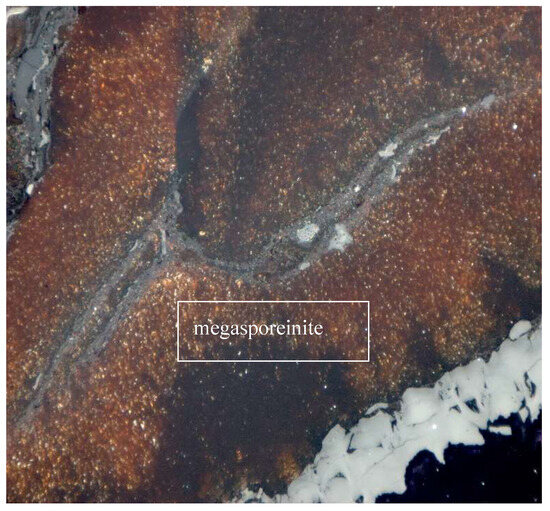
Figure 1.
Lipinite—megasporeinite. Oil immersion, magnification 500×.
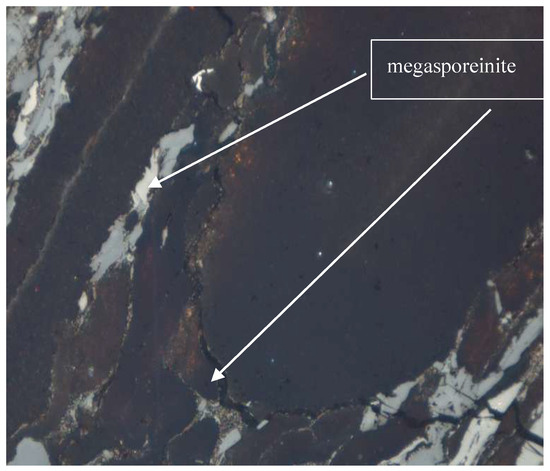
Figure 2.
Lipinite—megasporeinite. Oil immersion, magnification 500×.
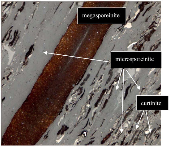
Figure 3.
Lipinite—megasporeinite, microsporeinite and curtinite. Oil immersion, magnification 500×.
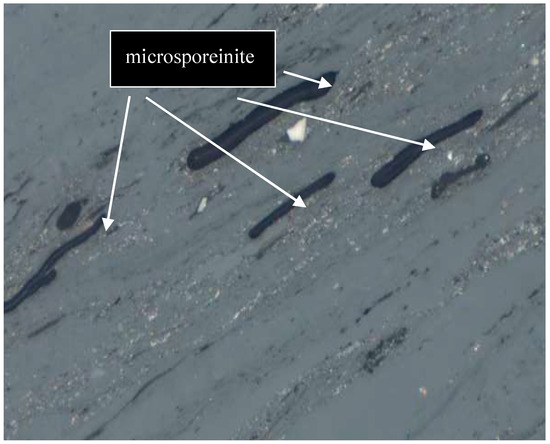
Figure 4.
Liptynite—microsporeinite. Oil immersion, magnification 500×.
Cutinite, on the other hand, represents leaf epithelium (cuticle) or needle epithelium as presented in Figure 3 and Figure 5. The upper leaf cuticle is thicker and serrated on one side, while the lower leaf cuticle is thinner and has slits. In reflected light, the color of cutinite is dark gray to light gray.
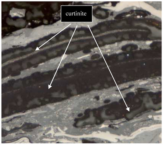
Figure 5.
Lipinite—curtinite. Oil immersion, magnification 500×.
Resinite is formed from plant resins and essential oils transformed into resins. It occurs very rarely in hard coals. Most often in the form of fillings of telinite cells, streaks, or lenses. In a microscopic image, in reflected light, it is dark gray and darker than sporanite and cutinite. It occurs very rarely.
The image processing and analyzing approach has been used with success in many applications, in fields such as biology, medicine, industry, and many others. There are also applications in discovering information on microscopic petrographic photographs [27]. The coal petrography and supporting discovery of solid fuels properties. The approach taken covers a wide area of ideas: from an investigation into a reflectance histogram, through the thresholding and segmentation based on color space [28], to the extensive use of color and texture features along with machine learning (ML) methods [29].
The Generative Adversarial networks (GAN) were used for resolution enhancement of coal microphotographs [25,30]. Usage of wide residual blocks along with multiscale attention allowed for obtaining more than satisfactory results. A very interesting attempt at using generative AI for enhancing and augmentation of training image sets was presented by Ma et al. [31]. The diffusion model was applied to generate artificial training images. The results were more than promising. The research of collotelinite (vitrinite) segmentation on microphotographs was made by Santos et al. [32]. The authors used Mask R-CNN for segmentation and then the reflectance of segmented maceral was determined by analyzing the gray level. There were reported applications of U-Net-based [33] architecture deep networks for macerals and intrusion detection on microphotographs [34,35,36]. Iwaszenko and Róg used a simplified U-Net architecture for maceral segmentation with good results for inertinite and vitrinite, and satisfactory (but not overwhelming) results for liptinite [34]. Fan et al. investigated the application of different modifications of U-Net for vitrinite, inertinite, and liptinite segmentation. The best results were obtained for U-Net with a ResNet [37] background and TransUNet [38,39]. However, the authors report liptinite as the most difficult maceral for segmentation. Wang et al. compared three different network architectures for semantic segmentation: U-Net, SegNet [40], and DeepLabV3+ [41]. The best results were achieved for the last architecture, and can be recognized as a reference for the automatic maceral groups segmentation.
Our work concentrates on liptinite segmentation on the microscopic images. The choice of liptinite as the only maceral group considered in the study was dictated by the observed difficulty in achieving an effective segmentation of it compared to other maceral groups (vitrinite, inertinite). Such a conclusion appears in previous works, although it is not always formulated directly [34,36,42]. In this paper, the focus is on U-type architecture. While networks of this type have been considered in previous works, the topic of studying their effectiveness in the context of liptinite appears to be open and promising for future research. The efficacy of networks based on this architecture in other applications suggests the potential for achieving high-fidelity segmentation of liptinite through the selection of network components and an appropriate training procedure. The research work carried out and presented in this article has confirmed this conjecture.
The selected deep network architectures based on U-Net were considered in the research, varying in depth and number of filters. The networks were trained “from scratch”, but commonly used backbone features extractors like ResNet were also examined (in different versions). An adjusted training procedure was proposed. The idea behind it was to pre-train the network from scratch using macerals easier to segment and then use them as initialization for liptinite segmentation.
2. Materials and Methods
2.1. Image Acquisition
For the purposes of this study, medium-sized samples for testing were taken in accordance with the ISO 18283:2006 standard Hard coal and coke—Manual sampling.
Samples of coal were obtained from the Polish Upper Silesian Coal Basin. The degree of carbonization of the organic substance of the collected coals, determined on the basis of the vitrinite reflectance index, did not exceed 0.75%.
Then, analytical samples with a grain size of less than 1 mm were prepared from the collected samples, from which microscopic briquettes were later prepared according to the PN-ISO standard ISO 7404-2:2009 Methods for the petrographic analysis of bituminous coal and anthracite—Part 2: Method of preparing coal samples.
Data on the tested coal samples (rank, the origin of the samples, and macerals compositions) are presented in Table 1. The microscopic specimens were prepared via immersion of coal dust in a mixture of epoxy resin and hardener, obtained by mixing the components in a ratio of 8:1. The immersed microscopic specimens were left for at least 24 h until solidification. The solidified specimens were polished using a Struers LaboForce-3 grinding/polishing machine.

Table 1.
Data on the tested coal samples.
A Zeiss Axio Imager Z 2 m microscope (Figure 6) was used for the study. A magnification of 500 times and white light reflected in oil immersion (refractive index n = 1.5180) were used. Surfaces, on which the photographs were taken using an Axiocam 506 color camera, were selected. The set of microscope photographs obtained shows different macerals from the liptinite group, for which a mask set was developed. In the petrographic analysis, the participation of macerals groups is most important.
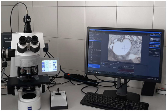
Figure 6.
Microscope Zeiss Axio Imager Z 2 m.
2.2. Images Preprocessing
Gathered visual information originated from two different microscopes (see section above). The sizes of acquired images varied from 1600 × 1200 pixels to 2752 × 2208 pixels. All images represented were taken with the same magnification—500×. To unify the input image dataset, all images were rescaled so that the width remained at 1600 pixels. Such resizing ensured the same size of the sample area represented by one pixel, with a size of 0.15652 × 0.15652 μm. Rescaling was performed using a Lanczos resampler [43]. No exposure corrections were made. Then, the image set was split into square tiles 512 × 512 pixels each. The resulting input set consisted of 590 images. It was divided into training and test sets in the proportion of 4:1. The images were normalized to fit the 0–1 interval. The normalization was performed per channel.
2.3. Training Procedure
The training procedure used images from the training set. To mitigate the overfitting and increase the trained networks’ generalization capabilities, an augmentation technique was used. However, the augmentation operations were limited to the operations that did not require image re-rasterization. Moreover, emphasis was placed on the use of transformations that could potentially generate images similar to those obtained during the image acquisition process. Say the transformations were chosen from the following set:
- Horizontal flip;
- Vertical flip;
- Rotation by angle 90°, 180°, 270°;
During the training phase, each image was subjected to one of the aforementioned transformations. The specific transformation was selected at random. Subsequently, with a probability of 0.5, the image underwent the transformation or remained unchanged. Depending on the experiment, the images were rescaled to 256 × 256 pixels or left in their original size (512 × 512). For the augmentation workflow, the Albumentations open-source library was used [44]. The testing set was not augmented in any way.
The training procedure assumed training the model for an arbitrarily chosen number of epochs. A series of preliminary experiments were conducted to determine the range of epochs that would yield the anticipated outcomes. The underlying assumption was that a point would be reached at which the network would exhibit indications of overfitting, as evidenced by the discrepancy in loss, IoU, and accuracy between training and test image sets. The findings indicated that, in our particular case, 800 epochs constituted the optimal training range. There were no automatic early stopping conditions applied. During the training, the binary cross entropy loss function was used:
where stands for the loss function, , are true and predicted class (, , and N is the batch size. As the input dataset was unbalanced (there were much more pixels belonging to the background than to the liptinite), the weighted form of the binary cross entropy function was used. The model quality was assessed using two measures: IoU (Intersection over Union—Jaccard index) and accuracy:
The symbol denote a set of pixels representing ground truth on an image, while the symbol represents the set of image pixels classified as belonging to the sought object by the segmentation model. Similarly, the symbols TP, TN, FP, FN are true positive (foreground pixel classified as foreground), true negative (background pixel classified as background), false positive (background pixel classified as foreground), and false negative (foreground pixel classified as background). The value used for estimating the effectiveness of the model is the average computed on all images from the test set.
The ADAM [45] algorithm was used for loss function minimization. During training, two strategies for the learning rate value estimation were considered. The first assumed keeping the learning rate value constant during the training process, while the second lowered the learning rate by half every 100 epochs. Loss function, accuracy, and IoU were monitored for both training and test sets during training procedure.
2.4. Deep Network Architectures
The research was focused on a deep convolutional networks, belonging to the U-Net-originating networks family. The base U-Net network, previously designed for medical images semantic segmentation, consists of two branches: an encoder and a decoder. The important architecture detail, which differs U-Net from other encoder–decoder architectures is the existence of so-called skip connections: the links between corresponding layers in the encoder and decoder parts. They are responsible for transferring, in the form of feature maps, the spatial information from the encoder to the decoder, which would be lost otherwise. The conducted research considered the following architectures:
- U-Net (three variants with varying depths were examined);
- U-Net with channel attention (three variants with varying depths were examined);
- U-Net with ResNet backbone (five variants of ResNet backbones were examined).
A detailed description of the network architectures is presented in the subsections below. Each deep network variant was trained for squared tiles of sizes 512 × 512 pixels and 256 × 256 pixels. In the case of larger resolutions, no resizing was applied to the input data, while the smaller ones were resized versions of the bigger ones. Differentiations of the tile sizes were aimed at investigating potential resizing and resolution influence on segmentation results.
2.4.1. U-Net Architecture
The architecture of the used U-Net deep network is depicted in Figure 7. Both encoder and decoder parts extensively use convolutional neural networks. For the experiments, the depth of the network was changed from 4 to 6 sections composing the encoder and decoder blocks. The number of filters started at 16 on the shallowest layer, going up to 128, 256, and 512 in the deepest one (depending on the tested network depth). ReLU activation was used everywhere except the network output, where the sigmoid function was used instead. The overall depth of the network was lower than that originally proposed by Ronneberger [33]. The limitation was applied because of the size of the input image—at each level, the size of feature maps was halved in each dimension, so the deepest feature maps’ size determined the reasonable depth of the network.
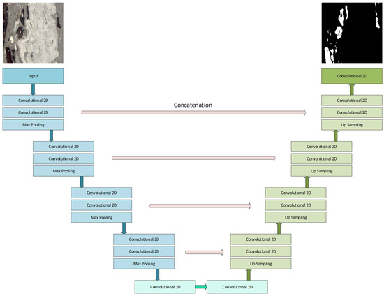
Figure 7.
U-Net deep network architecture.
2.4.2. U-Net with Channel Attention Architecture
For checking if slight attention can have an observable effect on liptinite segmentation effectiveness, a simple mechanism for channel-wise attention was proposed. The architecture of the network was modified on the concatenation paths by adding a vector of trainable weights. The weights were supposed to favor some of the concatenated feature maps while inhibiting the others. The structure of the proposed mechanism is depicted in Figure 8. Similarly to the case described in the previous section, three depths of the network were considered (from 128 to 512 filters in the deepest layer). The proposed attention mechanism is simple. At each level of the U-Net structure, the features maps, before concatenating with the corresponding layer in the decoder branch, were multiplied by a vector of attention coefficients α:
where is a tensor of features at level i, is the resulting tensor of features, and is attention coefficients vector for layer i. The operator is a multiplication—each features map from the features tensor is multiplied by the corresponding element of the attention coefficients’ vector (the operator resembles the well-known Hadamard product). The attention coefficients vector is subject to training.
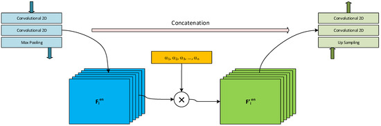
Figure 8.
U-Net with simple attention—the idea of the attention mechanism was used. The attention coefficients, α1, α2, …, αn, are used for the multiplication of the feature maps (each coefficient is used for the whole map, no spatial attention is used).
2.4.3. U-Net with ResNet Backbone Architecture
The third of the investigated architectures used the encoder build with the usage of ResNet blocks. The encoder branch in each architecture consisted of four ResNet blocks, while the decoder had the same construction as the first and second architectures (up-sampling and convolutional layers). There were five different U-Net—ResNet configurations, which differed with the type of ResNet blocks used: ResNet18, ResNet34, ResNet50, ResNet101, and ResNet152. In each case, pre-trained ResNet parts were used. However, they were not frozen, and their weights were modified during training.
The complete list of deep network architectures is presented in Table 2 Each of the networks was subject to training with the 256 × 256 resolution, as well as the 512 × 512 resolution, with the same procedure. All networks were implemented using pytorch. The computations were conducted on PC running a Microsoft Windows operating system. The computer was equipped with an Intel Core i7-12700H 2.70 GHz processor, 32 GB of RAM, and NVIDIA RTX3080Ti, 16 GB VRAM graphics card.
Table 2.
Networks architectures used for liptinite segmentation experiments.
3. Results
The results present the best values obtained during the training procedure. First, the most effective approach to the training was established by the comparison of the results obtained with training using the constant learning rate coefficient to the scheduled learning rate training. The constant rate was chosen from the set of trials. The chosen value was different for the networks used, but fell between 10−3 and 10−4. For the scheduled learning rate corrections, the best results were achieved when the initial learning rate started with 10−3 and was halved every 100 epochs. In each case, the assumed number of epochs was equal to 800. However, when the signs of the lack of convergence were identified, the training was manually halted to conserve resources (only a few cases exhibited these characteristics). The results obtained for each of the networks and learning rate schedules are presented in Table 3. The typical charts presenting the loss function values were presented in Figure 9, and the values for IoU for such cases were presented in Figure 10. It can be observed that symptoms of overfitting are easier to spot on the IoU chart.
Table 3.
The results of liptinite segmentations for constant and scheduled learning rates.
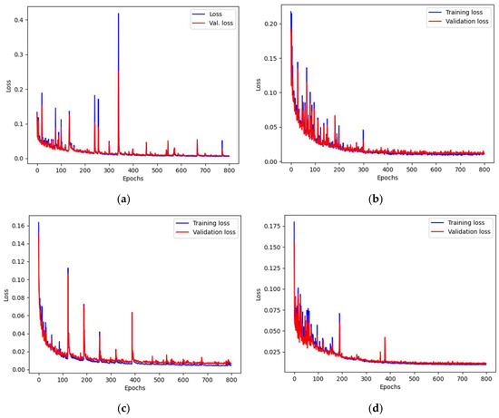
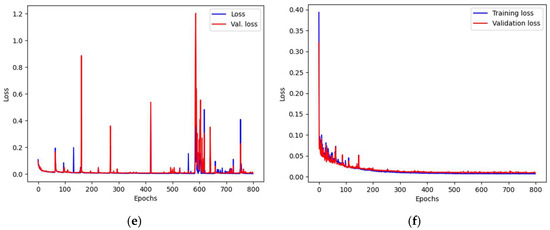
Figure 9.
The train and validation loss function values during model training. Charts (a,c,e) present the constant learning rate training, while charts (b,d,f) show the case of the scheduled learning rate approach. The architectures are as follows: (a,b) UN2; (c,d) SU2; (e,f) UR3. All networks were trained on 512 × 512 images.
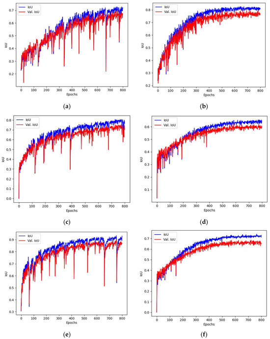
Figure 10.
The training and validation of IoU values during model training. Charts (a,c,e) present constant learning rate training, while charts (b,d,f) show the case of a scheduled learning rate approach. The architectures are as follows: (a,b) UN2; (c,d) SU2; (e,f) UR3. All networks were trained on 512 × 512 images.
The trained models were used for the computation of a set of segmentation quality measures. The IoU, acc (accuracy), rcl (recall), prc (precision), and F1 measures were used. The recall, precision, and F1 were calculated using the following formulas:
The obtained results are presented in Table 4. All measures were computed for each architecture as well as the image sizes. The table presents the best results achieved. For each model, the visualization of image segmentation was made for comparison with the ground truth. The typical segmentation results are depicted in Figure 11.
Table 4.
Network architectures and their best results. The best results in each column were marked in bold.
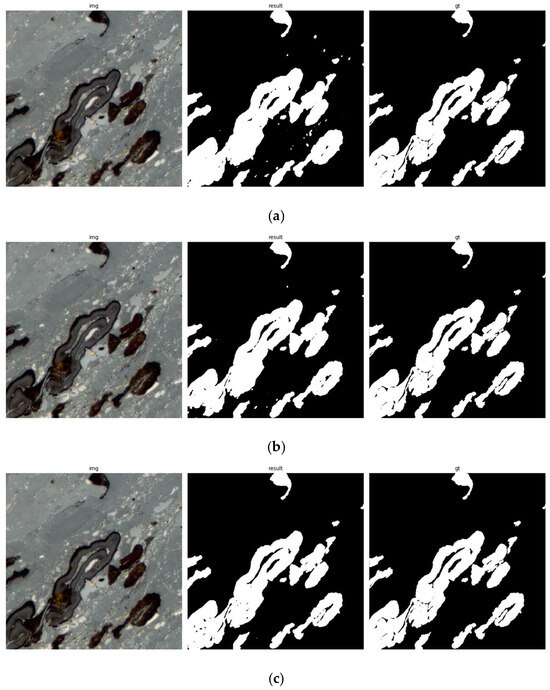
Figure 11.
The segmentation results for the selected trained networks: (a) UN2; (b) SU2; (c) UR3. All networks were trained on 512 × 512 images. The left column shows the input image, the right ground truth, and the middle segmentation results.
4. Discussion
In recent years, semantic segmentation has been a subject of research in the field of petrography [27,31,32,46]. Our research addresses the niche of petrography, important in the determination of the properties of coal, a sedimentary rock with a wide usage in the industry [47]. Our previous research [34] and other studies [29,36,42] show that vitrinite, liptinite, and inertinite expose various challenges for automatic segmentation. Among the three, liptinite was the most demanding and caused the most difficulties [34,36]. Therefore, the presented work focuses particularly on the liptinite, investigating the possibility of increasing the effectiveness of segmentation with the use of various deep network architectures (but still following the general U-Net architectural paradigm). In the following part of the discussion, the potential reasons for liptinite segmentation difficulties are considered, the influence of the network training protocol on the results is analyzed, and finally, the comparison of the achieved results with the results reported in the literature is presented.
4.1. Liptinite Segmentation Analysis
The liptinite was recognized as the most difficult one for segmentation out of all three maceral groups. Some of the researchers mention it directly [34,36], while in other research it can be observed in the measures used for segmentation description [42]. The hypothesis of the cause of the phenomenon was formulated by Fan et al. [36]. The authors postulate that the problem with segmentation is caused by its usual occurrence as worm-like structures on the vitrinite [5]. The other reason suggested is its lower presence compared to the other maceral groups, leading to a higher imbalance within the data, and therefore to difficulties in training. Following the presented hypothesis, the imbalance ratio was determined for the training set, yielding 11.218, which shows that the positive class (liptinite) is indeed in the vast minority. The imbalance problem was addressed by the application of weighted binary cross-entropy as a loss function:
where is the weight used for correcting the classes imbalance. The training procedure, with the loss function described by Equation (5), showed a much better convergence than the training with ordinary cross-entropy function [34]. The above is a point towards the confirmation of the hypothesis.
To further investigate the source of the possible poor performance of the proposed networks, the trained models were used to segment images from the test set, while simultaneous computations of the segmentation quality measures (IoU, acc, prc, rcl, F1) for each of the images. For each model, the worst cases were identified and analyzed. There were two crucial questions, for which answers were sought:
- Does the effectiveness of segmentation depend on network architecture?
- Are there any easily visible structure/texture properties that can explain the problems with segmentation?
If the answer to the first question is negative, worse performance should be observed for the same image no matter which network architecture is used, and the order of the images sorted according to the selected effectiveness measure should be almost the same for each model. Otherwise, if the network architecture is crucial for performance (its influence on performance is stronger than the image properties), it should be observed that both the worst-performing image, and the images’ order are strongly connected with the network architecture.
The investigations on the obtained data showed that, to a certain level, both effects can be observed. However, the dominant is the influence of the image itself. There were images causing problems for every network architecture tested. This is especially true for the images that resulted in the poorest segmentation. It seemed that these two images caused problems for every network architecture tested. The results for those images are presented in Figure 12. While more differences were observed for the subsequent problematic images, the group of the ‘difficult’ ones can be identified.
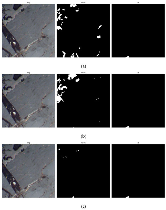
Figure 12.
The segmentation results for the most difficult image: (a) UN2; (b) SU2; (c) UR3. All networks were trained on 512 × 512 images. The left column shows the input image, the right shows the ground truth, and the middle shows the segmentation results. All network architectures performed poorly for the image, though the URx architectures struggled less.
Analyzing the results for the worst cases, it may be observed that most difficulties were caused by the images with only a tiny area occupied by segmented liptinite. The problems arose when the image structure was complicated—where there are many areas similar in shape and size, among which only one or two are actually liptinite. Though most of such images turned out to be difficult for segmentation for each architecture, it has to be noted that ResNet-based architectures performed better, even segmenting the image correctly, as presented in Figure 13. In general, the networks trained for higher-resolution images performed better.
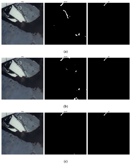
Figure 13.
The segmentation results for another difficult image: (a) UN2; (b) SU2; (c) UR3. All networks were trained on 512 × 512 images. The left column shows the input image, the right shows the ground truth, and the middle shows the segmentation results. The URx network’s result was much better than the other networks’.
4.2. Training Procedure Analysis
During the experiments, two training procedures were investigated and their influence on the results was analyzed. The first approach focused on networks trained using a constant learning rate, while during the second approach, the training rate was halved every 100 epochs. The value of the learning rate in the first approach was determined using a grid search. The training was limited to 200 epochs, and the used values formed a series of 10−2, 5 × 10⁻³, 10−3, 5 × 10⁻⁴, 10−4, 10−5. The selection criterium for the value used during further training was to achieve the highest IoU measure after 200 epochs. Once the starting value was established, it was used as the constant learning rate for the training for 800 epochs, and also as an initial value for the training using a scheduled learning rate. Taking into consideration that the ADAM optimizer performs the lr adaptation itself, the used learning rate established the range within which the adaptation was made [45]. The results show that generally comparable results can be achieved for both methods. However, elaborating on the correct value of the learning rate for the URx architectures turned out to be tricky. Either the low convergence or halting of learning was observed, depending on the value used. In the case of UNx and SUx, the effect was less prominent. It has to be pointed out that, during the training of RUx networks, the pre-trained ResNet backbones were used. However, the backbone was not frozen during the training, allowing for adjustment of its weights as necessary. In conclusion, it is more profitable to use learning rate scheduling than a constant value. It allows comparable results to training with constant lr. While it is still a question of how to choose the initial value and scheduling algorithm, it turned out to be less rigorous than in the case of constant lr.
4.3. Results Analysis
The results of the experiments show that the best results, in the IoU measure, were obtained for the networks with ResNet encoders. The results for the best architecture, UR3, trained on 512 × 512 images, were as high as 0.9156 in terms of IoU. The same network was also superior in terms of accuracy (0.9974) and F1 (0.9522). The obtained result was better than that achieved in earlier experiments. The results reported in [42], which can be used as a reference for the base values for the maceral identification, reveal the best IoU for liptinite at a level of 0.83. This value was obtained for DeepLabV3+ network. It is worth noting that none of “classic” U-Net architectures (UNx, SUx) were able to achieve better results. On the other hand, the networks with ResNet-based encoders were close to or better than this result. It is known from the literature that liptinite is more difficult to segment due to its form and visual properties in microscopic images [34,36,42]. Therefore, only more sophisticated architectures, with a greater ability for visual feature extraction proved to be successful in its segmentation. On the other hand, even the U-Net architectures can be expected to deliver reasonably good and practically usable results.
The application of a simple, map-oriented attention mechanism implemented in SUx networks turned out to be moderately successful. On the one hand, it allowed for achieving better results for almost all tested cases. On the other, the improvement was not good enough to overcome the results for the URx architectures or the best values reported for DeepLabV3+. Nevertheless, these networks are reasonably good at liptinite segmentation and efficient in terms of computation and memory requirements, so in cases where only limited hardware resources are available, they are still a good choice.
5. Conclusions
Identification of macerals in microscopic images is one of the methods of coal quality assessment. The process is usually difficult, and the involvement of experienced domain experts is crucial to achieve a good quality of the results. An attempt of using deep learning networks for the semantic segmentation of one of the maceral groups, the liptinite, was made. The liptinite was chosen as the most difficult for semantic segmentation. The U-Net-based architectures were used for the segmentation. Three groups of networks were examined: a classic U-Net architecture, but with a varying depth, a U-Net architecture with feature map simple attention mechanism implemented, and a U-Net architecture using a ResNet backbone in the encoder branch. The results show that the best results were achieved using the last approach, when the encoder was based on the ResNet50 network. The results were superior, and good enough to consider the architecture as a tool for potential automatic segmentation of liptinite. The other network architectures achieved worse results but were also much more efficient in terms of memory consumption and computation power requirements. The achieved results showed that even difficult macerals, such as liptinite can be effectively segmented using U-Net-based architectures. It was also shown that the most difficult images for the segmentation are those which contain a tiny amount of liptinite in them. Only the most complex architectures (ResNet-based) were capable of successfully segmentingsuch cases. In the case of this particular architecture, the best value of the IoU measure observed was equal to 0.91. The presented results can justify stating that the domain experts can be effectively supported by computer vision tools in the identification and segmentation of maceral groups in microscopic images.
Author Contributions
Conceptualization, S.I. and L.R.; methodology, S.I. and L.R.; software, S.I.; validation, S.I. and L.R.; formal analysis, S.I.; investigation, S.I.; resources, L.R.; data curation, S.I.; writing—original draft preparation, S.I. and L.R.; writing—review and editing, S.I.; visualization, S.I.; supervision, S.I.; project administration, L.R.; funding acquisition, L.R. All authors have read and agreed to the published version of the manuscript.
Funding
This research was funded by the Ministry of Science and Higher Education, Republic of Poland, grant number 111 85011 (Statutory Activity of the GIG National Research Institute).
Data Availability Statement
The data presented in this study are available on request from the corresponding author due to proprietary data are used in the research.
Conflicts of Interest
The authors declare no conflicts of interest.
References
- Dai, S.; Hower, J.C.; Finkelman, R.B.; Graham, I.T.; French, D.; Ward, C.R.; Eskenazy, G.; Wei, Q.; Zhao, L. Organic Associations of Non-Mineral Elements in Coal: A Review. Int. J. Coal Geol. 2020, 218, 103347. [Google Scholar] [CrossRef]
- Hower, J.C.; Eble, C.F.; O’Keefe, J.M. Phyteral Perspectives: Every Maceral Tells a Story. Int. J. Coal Geol. 2021, 247, 103849. [Google Scholar] [CrossRef]
- for Coal, I.C. The New Vitrinite Classification (ICCP System 1994). Fuel 1998, 77, 349–358. [Google Scholar]
- Sỳkorová, I.; Pickel, W.; Christanis, K.; Wolf, M.; Taylor, G.; Flores, D. Classification of Huminite—ICCP System 1994. Int. J. Coal Geol. 2005, 62, 85–106. [Google Scholar] [CrossRef]
- Pickel, W.; Kus, J.; Flores, D.; Kalaitzidis, S.; Christanis, K.; Cardott, B.; Misz-Kennan, M.; Rodrigues, S.; Hentschel, A.; Hamor-Vido, M.; et al. Classification of Liptinite–ICCP System 1994. Int. J. Coal Geol. 2017, 169, 40–61. [Google Scholar] [CrossRef]
- Kruszewska, K.; Dybowa-Jachowicz, S. Draft of Coal Petrology; Publishing House of the University of Silesia: Katowice, Poland, 1997. [Google Scholar]
- O’Keefe, J.M.; Bechtel, A.; Christanis, K.; Dai, S.; DiMichele, W.A.; Eble, C.F.; Esterle, J.S.; Mastalerz, M.; Raymond, A.L.; Valentim, B.V.; et al. On the Fundamental Difference between Coal Rank and Coal Type. Int. J. Coal Geol. 2013, 118, 58–87. [Google Scholar]
- Parzentny, H.R.; Róg, L. Dependences between Certain Petrographic, Geochemical and Technological Indicators of Coal Quality in the Limnic Series of the Upper Silesian Coal Basin (USCB), Poland. Arch. Min. Sci. 2020, 65, 665–684. [Google Scholar]
- de Vasconcelos, L.S. The Petrographic Composition of World Coals. Statistical Results Obtained from a Literature Survey with Reference to Coal Type (Maceral Composition). Int. J. Coal Geol. 1999, 40, 27–58. [Google Scholar] [CrossRef]
- Denge, E.; Baiyegunhi, C. Maceral Types and Quality of Coal in the Tuli Coalfield: A Case Study of Coal in the Madzaringwe Formation in the Vele Colliery, Limpopo Province, South Africa. Appl. Sci. 2021, 11, 2179. [Google Scholar] [CrossRef]
- Suárez-Ruiz, I.; Ward, C.R. Basic Factors Controlling Coal Quality and Technological Behavior of Coal. In Applied Coal Petrology; Elsevier: Amsterdam, The Netherlands, 2008; pp. 19–59. [Google Scholar]
- Cutruneo, C.M.; Oliveira, M.L.; Ward, C.R.; Hower, J.C.; de Brum, I.A.; Sampaio, C.H.; Kautzmann, R.M.; Taffarel, S.R.; Teixeira, E.C.; Silva, L.F. A Mineralogical and Geochemical Study of Three Brazilian Coal Cleaning Rejects: Demonstration of Electron Beam Applications. Int. J. Coal Geol. 2014, 130, 33–52. [Google Scholar] [CrossRef]
- Méndez, L.; Borrego, A.; Martinez-Tarazona, M.; Menéndez, R. Influence of Petrographic and Mineral Matter Composition of Coal Particles on Their Combustion Reactivity. Fuel 2003, 82, 1875–1882. [Google Scholar] [CrossRef]
- Jelonek, I.; Jelonek, Z. The Influence of Petrographic Properties of Bituminous Coal on the Quality of Metallurgical Coke. Zesz. Nauk. Inst. Gospod. Surowcami Miner. Pol. Akad. Nauk 2017, 100, 49–65. [Google Scholar]
- Jelonek, I.; Mirkowski, Z. Petrographic and Geochemical Investigation of Coal Slurries and of the Products Resulting from Their Combustion. Int. J. Coal Geol. 2015, 139, 228–236. [Google Scholar] [CrossRef]
- Bielowicz, B. Petrographic Characteristics of Coal Gasification and Combustion By-Products from High Volatile Bituminous Coal. Energies 2020, 13, 4374. [Google Scholar] [CrossRef]
- Fender, T.D.; Rouainia, M.; Van Der Land, C.; Jones, M.; Mastalerz, M.; Hennissen, J.A.; Graham, S.P.; Wagner, T. Geomechanical Properties of Coal Macerals; Measurements Applicable to Modelling Swelling of Coal Seams during CO2 Sequestration. Int. J. Coal Geol. 2020, 228, 103528. [Google Scholar] [CrossRef]
- Misra, B.K.; Singh, B.D. Liptinite Macerals in Singrauli Coals, India: Their Characterization and Assessment. J. Palaeosci. 1993, 42, 1–13. [Google Scholar] [CrossRef]
- Kruszewska, K.; Szwed-Lorenz, J. Petrographic Basis of the Variability of Coal Quality in Deposit. Sci. Pap. Silesian Univ. Technol. 2005, 268. [Google Scholar]
- Hower, J.C.; Ban, H.; Schaefer, J.L.; Stencel, J.M. Maceral/Microlithotype Partitioning through Triboelectrostatic Dry Coal Cleaning. Int. J. Coal Geol. 1997, 34, 277–286. [Google Scholar] [CrossRef]
- Bielowicz, B. Petrographic Composition of Coal from the Janina Mine and Char Obtained as a Result of Gasification in the CFB Gasifier. Gospod. Surowcami Miner.-Miner. Resour. Manag. 2019, 35, 99–116. [Google Scholar] [CrossRef]
- Bielowicz, B.; Misiak, J. The Impact of Coal’s Petrographic Composition on Its Suitability for the Gasification Process: The Example of Polish Deposits. Resources 2020, 9, 111. [Google Scholar] [CrossRef]
- Róg, L. Vitrinite Reflectance as a Measure of the Range of Influence of the Temperature of a Georeactor on Rock Mass during Underground Coal Gasification. Fuel 2018, 224, 94–100. [Google Scholar] [CrossRef]
- Mirkowski, Z.; Jelonek, I. Petrographic Composition of Coals and Products of Coal Combustion from the Selected Combined Heat and Power Plants (CHP) and Heating Plants in Upper Silesia, Poland. Int. J. Coal Geol. 2019, 201, 102–108. [Google Scholar] [CrossRef]
- Jasieńko, S.; Róg, L. Pertographic Constitution, Physical, Chemical and Technological Properties of the Fractions Separated from Flame Coal and Gas Flame Coal Using Enrichment in Heavy Liquids. Int. Conf. Coal Sci. 1993, 1, 377–380. [Google Scholar]
- Jasienko, S.; Róg, L. Petrographic Constitution, Physical, Chemical and Technological Properties of the Fractions Isolated from Metacoking Coal and Semicoking Coal by the Method of Separation in Heavy Liquids. Coal Sci.-Proc. Eighth Int. Conf. Coal Sci. 1995, 24, 263–266. [Google Scholar]
- Saxena, N.; Day-Stirrat, R.J.; Hows, A.; Hofmann, R. Application of Deep Learning for Semantic Segmentation of Sandstone Thin Sections. Comput. Geosci. 2021, 152, 104778. [Google Scholar] [CrossRef]
- Jiu, B.; Huang, W.; Shi, J.; Hao, R. A Method to Extract the Content, Radius and Specific Surface Area of Maceral Compositions in Coal Reservoirs Based on Image Modeling. J. Pet. Sci. Eng. 2021, 201, 108419. [Google Scholar] [CrossRef]
- Skiba, M.; Młynarczuk, M. Identification of Macerals of the Inertinite Group Using Neural Classifiers, Based on Selected Textural Features. Arch. Min. Sci. 2018, 63, 827–837. [Google Scholar] [CrossRef]
- Zou, L.; Xu, S.; Zhu, W.; Huang, X.; Lei, Z.; He, K. Improved Generative Adversarial Network for Super-Resolution Reconstruction of Coal Photomicrographs. Sensors 2023, 23, 7296. [Google Scholar] [CrossRef]
- Ma, Z.; He, X.; Kwak, H.; Gao, J.; Sun, S.; Yan, B. Enhancing Rock Image Segmentation in Digital Rock Physics: A Fusion of Generative Ai and State-of-the-Art Neural Networks. arXiv 2023, arXiv:2311.06079. [Google Scholar]
- Santos, R.B.M.; Augusto, K.S.; Iglesias, J.C.Á.; Rodrigues, S.; Paciornik, S.; Esterle, J.S.; Domingues, A.L.A. A Deep Learning System for Collotelinite Segmentation and Coal Reflectance Determination. Int. J. Coal Geol. 2022, 263, 104111. [Google Scholar] [CrossRef]
- Ronneberger, O.; Fischer, P.; Brox, T. U-Net: Convolutional Networks for Biomedical Image Segmentation. In Proceedings of the International Conference on Medical Image Computing and Computer-Assisted Intervention, Munich, Germany, 5–9 October 2015; Springer: Berlin/Heidelberg, Germany, 2015; pp. 234–241. [Google Scholar]
- Iwaszenko, S.; Róg, L. Application of Deep Learning in Petrographic Coal Images Segmentation. Minerals 2021, 11, 1265. [Google Scholar] [CrossRef]
- Iwaszenko, S.; Szymańska, M.; Róg, L. A Deep Learning Approach to Intrusion Detection and Segmentation in Pellet Fuels Using Microscopic Images. Sensors 2023, 23, 6488. [Google Scholar] [CrossRef] [PubMed]
- Fan, J.; Du, M.; Liu, L.; Li, G.; Wang, D.; Liu, S. Macerals Particle Characteristics Analysis of Tar-Rich Coal in Northern Shaanxi Based on Image Segmentation Models via the U-Net Variants and Image Feature Extraction. Fuel 2023, 341, 127757. [Google Scholar] [CrossRef]
- He, K.; Zhang, X.; Ren, S.; Sun, J. Deep Residual Learning for Image Recognition. In Proceedings of the IEEE Conference on Computer Vision and Pattern Recognition, Las Vegas, NV, USA, 27–30 June 2016; pp. 770–778. [Google Scholar]
- Chen, J.; Lu, Y.; Yu, Q.; Luo, X.; Adeli, E.; Wang, Y.; Lu, L.; Yuille, A.L.; Zhou, Y. Transunet: Transformers Make Strong Encoders for Medical Image Segmentation. arXiv 2021, arXiv:2102.04306. [Google Scholar]
- Fang, J.; Yang, C.; Shi, Y.; Wang, N.; Zhao, Y. External Attention Based TransUNet and Label Expansion Strategy for Crack Detection. IEEE Trans. Intell. Transp. Syst. 2022, 23, 19054–19063. [Google Scholar] [CrossRef]
- Badrinarayanan, V.; Kendall, A.; Cipolla, R. Segnet: A Deep Convolutional Encoder-Decoder Architecture for Image Segmentation. IEEE Trans. Pattern Anal. Mach. Intell. 2017, 39, 2481–2495. [Google Scholar] [CrossRef] [PubMed]
- Yang, Z.; Peng, X.; Yin, Z. Deeplab_v3_Plus-Net for Image Semantic Segmentation with Channel Compression. In Proceedings of the 2020 IEEE 20th International Conference on Communication Technology (ICCT), Nanning, China, 28–31 October 2020; IEEE: New York, NY, USA, 2020; pp. 1320–1324. [Google Scholar]
- Wang, Y.; Bai, X.; Wu, L.; Zhang, Y.; Qu, S. Identification of Maceral Groups in Chinese Bituminous Coals Based on Semantic Segmentation Models. Fuel 2022, 308, 121844. [Google Scholar] [CrossRef]
- Turkowski, K. Filters for Common Resampling Tasks. In Graphics Gems; Academic Press Inc.: Cambridge, MA, USA, 1990; pp. 147–165. [Google Scholar]
- Buslaev, A.; Parinov, E.; Khvedchenya, E.; Iglovikov, V.I.; Kalinin, A.A. Albumentations: Fast and Flexible Image Augmentations. arXiv 2018, arXiv:1809.06839. [Google Scholar] [CrossRef]
- Kingma, D.P.; Ba, J. Adam: A Method for Stochastic Optimization. arXiv 2017, arXiv:1412.6980. [Google Scholar]
- Ye, P.; Yu, B.; Zhang, R.; Chen, W.; Li, Y. Development and Application of a More Refined Process for Extracting Rock Crack Width Information Based on Artificial Intelligence. Res. Sq. 2023. [Google Scholar]
- Voncken, J. The Origin and Classification of Coal. In Geology of Coal Deposits of South Limburg, The Netherlands; Springer: Berlin/Heidelberg, Germany, 2020; pp. 25–40. ISBN 978-1-4939-8930-0. [Google Scholar]
Disclaimer/Publisher’s Note: The statements, opinions and data contained in all publications are solely those of the individual author(s) and contributor(s) and not of MDPI and/or the editor(s). MDPI and/or the editor(s) disclaim responsibility for any injury to people or property resulting from any ideas, methods, instructions or products referred to in the content. |
© 2025 by the authors. Licensee MDPI, Basel, Switzerland. This article is an open access article distributed under the terms and conditions of the Creative Commons Attribution (CC BY) license (https://creativecommons.org/licenses/by/4.0/).