Machine Learning Approaches for Predicting the Elastic Modulus of Basalt Fibers Combined with SHapley Additive exPlanations Analysis

Abstract

The elastic modulus of basalt fibers is closely associated with their chemical composition. In this study, eight machine learning models were developed to predict the elastic modulus, with hyper-parameter tuning implemented through the GridSearchCV technique. Model performance was evaluated using the coefficient of determination (R²), root-mean-square error (RMSE), and mean absolute error (MAE). SHAP analysis was employed to uncover the relevance of oxide compositions and their interactions with the elastic modulus. Among these models, the Categorical Boosting algorithm exhibited the best results, with an R² of 0.9554, an RMSE of 4.7556, and an MAE of 2.0323. SHAP analysis indicated that CaO had the most significant influence on elastic modulus predictions. The importance of other oxides was ranked as follows: SiO₂, Al₂O₃, MgO, K₂O, Na₂O, Fe₂O₃, FeO, and TiO². Additionally, SHAP analysis determined oxide ranges for positive elastic modulus prediction. This research provides new insights into leveraging machine learning to optimize the mechanical properties of basalt fibers.

1. Introduction

Basalt fibers, recognized as a high-performance fiber material, have gained considerable attention for their superior mechanical strength, thermal resistance, and commendable chemical stability [1]. These fibers are produced from natural basalt rocks through a melt-spinning process and comprise chemicals like SiO₂, Al₂O₃, CaO, MgO, FeO, and Fe₂O₃ [2]. The elastic modulus of basalt fibers denotes the ratio of incremental stress to incremental strain during the phase of elastic deformation when the fiber is subjected to external force [3,4]. This ratio serves as a critical indicator of the basalt fiber’s rigidity and capacity to resist deformation under stress. In scenarios requiring the endurance of high loads, such as high-strength composite materials [5,6] and reinforced concrete [7,8], a high elastic modulus is essential. Furthermore, the advantages of basalt fibers, including their low production costs [9] and eco-friendliness [10], render them a compelling substitute for reinforcement materials in various industrial applications.

Basalt fiber-reinforced composites are produced by adding basalt fibers as reinforcement into the matrix of composite materials. These reinforced composites include basalt fiber-reinforced cement and basalt fiber-reinforced polymer composites [11], which generally exhibit excellent mechanical properties, chemical stability, and durability [12]. Tumadhir et al. analyzed the elastic modulus of basalt fiber-reinforced concrete with different basalt fiber volume fractions (0.1%, 0.2%, 0.3%, and 0.5%) [13]. The results indicated that the elastic modulus reached its maximum value at a volume fraction of 0.3%. Ayub et al. discovered that the elastic modulus of concrete increases with the addition of basalt fiber volume fraction, with the optimal basalt fiber content being between 1% and 3% [14]. Elmahdy et al. conducted research on the elastic modulus of basalt and glass–epoxy composites under various strain rates. Across all tested strain rates, the elastic modulus of basalt–epoxy composites surpassed that of glass–epoxy composites, with a difference ranging from 3.7% to 41% [14]. In a comparative study by Lopresto et al., the Young’s modulus of basalt composites was found to be 45% higher than glass composites [15]. Obviously, the elastic modulus of basalt fiber has a significant effect on the elastic modulus of reinforced composites.

Previous studies have shown that the elastic modulus of basalt fibers is closely related to their chemical composition. The primary chemical composition of SiO₂, Al₂O₃, CaO, MgO, FeO, and Fe₂O₃ has various effects on the lattice structure, which, in turn, affects the elastic modulus of the basalt fibers and, consequently, the mechanical properties of basalt-reinforced composites. Ding et al. compared the elastic modulus of basalt fibers and glass fibers, finding that the elastic modulus of basalt fibers is approximately 18% higher than that of glass fibers [16]. Research from Deák et al. shown that SiO₂ and Al₂O₃ are the main components of basalt fibers, and increasing their content can enhance the elastic modulus of basalt fibers [17]. The sum of the content of SiO₂ and Al₂O₃ has a high correlation with the elastic modulus of basalt fibers, with a correlation coefficient of up to 0.80. Oxides formed from ions with a greater ionic radius and lower charges, like Na⁺, K⁺, and Ba²⁺, do not favor the enhancement of the elastic modulus. On the other hand, oxides consisting of ions with a smaller ionic radius and higher polarization abilities, such as Li⁺, Be²⁺, Mg²⁺, AI³⁺, and Ti⁴⁺, contribute to an increased elastic modulus [18].

Machine learning is an effective tool for predicting the mechanical properties of basalt-reinforced materials and reinforced concrete. Wei et al. utilized an Artificial Neural Network (ANN) model to predict the alkali resistance of basalt fibers. The input variables for the model included the content of Si, Al, Fe, Ca, Mg, K, Na, Ti, and Zr in both basalt and glass fibers, with the output variable being the tensile strength retention rate. The optimized ANN model achieved an R² value of 0.92 on the test set [19]. Sun et al. developed three different eXtreme Gradient Boosting (XGBoost) models to predict the split tensile strength of basalt fiber-reinforced coral aggregate concrete. The ESOA-XGBoost (egret swarm optimization XGBR) performed best, with an R² of 0.9633 [20]. Alarfaj et al. compared the performance of five machine learning models in predicting the splitting tensile strength of fiber-reinforced recycled aggregate concrete, and the deep neural network showed the best performance, with the highest R² value of 0.94 [21]. A review study by Machello et al. found that various machine learning algorithms can generally predict the mechanical properties of fiber-reinforced polymer (FRP) composites accurately with minimal error. It also pointed out that more experimental data are needed in future studies to enhance the current database and improve the performance of these machine learning models [22]. It is clear that machine learning can be used to reveal the relationship between the chemical composition of basalts and their elastic modulus.

This study evaluates the performance of eight machine learning models (Multiple Linear Regression (MLR), K-Nearest Neighbors (KNN), decision tree (DT), Support Vector Regression (SVR), and ANN, as well as ensemble machine learning models such as Random Forest (RF, based on the Bagging algorithm), XGBoost (based on the Boosting algorithm), and Categorical Boosting (CatBoost, based on the Boosting algorithm)) in predicting the elastic modulus of basalt fibers. The chemical components SiO₂, Al₂O₃, TiO₂, Fe₂O₃, CaO, Na₂O, MgO, FeO, and K₂O are used as input variables, with the elastic modulus as the output variable. The coefficient of determination (R²), root-mean-square error (RMSE), and mean absolute error (MAE) serve as evaluation metrics for assessing the predictive accuracy of the models. SHapley Additive exPlanations (SHAP) is applied to analyze the significance of each input variable in the optimal model and the dependence relationship between variables. This study presents a cost-effective and efficient approach for predicting the mechanical properties of basalt fibers based on their chemical composition, showcasing the potential of machine learning in the industrial production of basalt fibers.

2. Materials and Methods

2.1. Data Pre-Processing

The data utilized in this study comprise experimental and literature data. Among them, 92 sets of experimental data were provided by Sichuan Sizhong Basalt Fiber Technology Research Co., Ltd. The remaining 85 literature datasets were primarily sourced from studies published between 2008 and 2023 [16,17,23,24,25,26,27,28,29,30,31,32,33,34,35,36,37,38,39,40,41,42], retrieved through keyword combinations (“chemical composition” with “basalt fiber” or “basalt”) in Elsevier, Springer, Wiley, and related databases. This timeframe was selected to analyze recent advancements in the study of elastic modulus of basalt fiber and its chemical composition, as well as to explore the relationship between them. All literature data were entirely based on peer-reviewed publications focused on the chemical compositions of basalt and their corresponding fiber strengths. The data comprised input variables and output variables. The input variables encompassed the chemical components of SiO₂, Al₂O₃, TiO₂, Fe₂O₃, CaO, Na₂O, MgO, FeO, and K₂O, while the output variable was the elastic modulus of basalt fibers. The chemical analyses predominantly employed Chemical analysis, ICP-OES, XRF, and EDS to quantify oxides. The elastic modulus of basalt fibers typically refers to the tangent modulus (Young’s Modulus) measured under uniaxial tension, following testing standards including ISO 9163:2005(E) [43], EN ISO 5079:1999 [44], the German standard DIN 65382 [45], GB/T 7690.1-2001 [46], GB/T 38897-2020 [47], GB/T3362-82 [48], ASTM C1557-14 [49], and ASTM D 3379-75 [50]. Analytical methods for chemical composition and elastic modulus in the literature are summarized in

Table A1. Analytical methods for chemical composition and elastic modulus in the literature.

Analytical Methods for Chemical Composition	Analytical Methods for Elastic Modulus	Fiber or Roving	References
Chemical analysis (ASTMC169-92)	ISO 9163:2005(E)	roving	[16]
ICP-OES	EN ISO 5079:1999	fiber	[17]
ICP-OES	German standard DIN 65382	fiber	[23]
EDS	GB/T 7690.1-7690.6-2001	fiber	[24]
XRF	ISO 5079	fiber	[25]
GB/T 1549-2008	GB/T 38897-2020	fiber	[26]
XRF	ISO 5079	fiber	[27]
Not mentioned	Not mentioned	fiber	[28]
XRF	ISO 5079	fiber	[29]
Not mentioned	Not mentioned	fiber	[30]
ICP	GB/T3362-82	roving	[31]
Not mentioned	Not mentioned	fiber	[32]
Not mentioned	Not mentioned	fiber	[33]
Not mentioned	Not mentioned	fiber	[34]
ICP	ASTM C1557–14	fiber	[35]
XRF	ASTM D 3379-75	fiber	[36]
Not mentioned	Not mentioned	fiber	[37]
Not mentioned	Not mentioned	fiber	[38]
Not mentioned	Not mentioned	fiber	[39]
Not mentioned	Not mentioned	fiber	[40]
XRF	Not mentioned	fiber	[41]
Not mentioned	Not mentioned	fiber	[42]

(Appendix B).

It should be noted that the adoption of different analytical methods (Chemical analysis, ICP-OES, XRF, and EDS) across literature studies indeed introduces systematic variations in measured chemical compositions, while the elastic modulus between single basalt and fiber rovings are indeed different, which may affect the development of machine learning models. However, because different testing methods were used in different studies, it was hard to unify the testing methods when collecting these data, which can lead to systematic variations in the measured values. Rigorous data cleaning was conducted on all collected data, which involved removing outliers and inputting missing values. Outlier removal was performed using the Z-score method, through which outliers were identified and eliminated from the dataset. The Z-score for each data point was calculated using the formula

$$\mathrm{Z}={\displaystyle \frac{x-\mu }{\sigma }}$$

(1)

where $x$ represents the data point, $\mu$ is the mean of the dataset, and $\sigma$ is the standard deviation. A threshold of $\mathrm{Z}$ > 3 was set, meaning any data point with a $\mathrm{Z}$-score greater than 3 or less than −3 was classified as an outlier and excluded from the analysis. This threshold was selected based on field-specific conventions and dataset characteristics. The missing values were imputed with the mean value of the remaining variables, which is a commonly adopted method. Following data cleaning, the input variables were standardized, namely normalized to the range of [0, 1], to ensure that all data were on the same scale.

2.2. Machine Learning Models

Representative machine learning models including MLR, KNN, DT, SVR, ANN, RF, XGBoost, and CatBoost were selected for training and testing in this study. An overview of each model’s algorithm, along with its basic principles, advantages, and disadvantages, is provided in Appendix A.

2.3. Hyper-Parameter Optimization

The empirical results suggest that for traditional machine learning applications with limited datasets (e.g., sample sizes below 10,000), a 70:30 training–test split often achieves optimal balance, enabling reliable evaluation of model generalizability. Therefore, the preprocessed data were divided into a training set (70%) and a testing set (30%) to ensure that the models could perform well on unseen data. GridSearchCV was employed for hyper-parameter optimization of each machine learning model. This method involves setting a series of candidate hyper-parameter values and combining them with cross-validation to identify the optimal combination of hyper-parameters that maximizes model performance. This step is crucial for improving the generalization ability and prediction accuracy of the models.

2.4. Model Performance Evaluation

The evaluation metrics R², RMSE, and MAE were employed to compare the performance of the model on both the training and testing sets after hyper-parameter optimization. These metrics provide a comprehensive evaluation of the model’s predictive accuracy and stability. R² provides an overall measure of model performance, while RMSE and MAE offer more specific indications of the magnitude of prediction errors. The coefficient of determination, R², primarily assesses the degree of fit between the model predicted values and the actual observed values, with a value closer to 1 indicating a better fit of the model.

$$R^2=1-{\displaystyle \frac{SSE}{SST}}$$

(2)

SSE (Sum of Squares due to Error) represents the sum of squared residuals, which is the sum of the squares of the differences between the predicted values and the actual observed values. SST (Total Sum of Squares) denotes the total sum of squared deviations, which is the sum of the squares of the differences between the actual observed values and their mean. The coefficient of determination can also be expressed by the following formula.

$$R^2=1-{\displaystyle \frac{\sum _{i=1}^m{(y_i-{\widehat{y}}_i)}^2}{\sum _{i=1}^m{(y_i-{\overline{y}}_i)}^2}}$$

(3)

RMSE is the square root of the ratio of the sum of the squared deviations between the observed values and the actual observed values to the number of observations, m.

$$\mathrm{R}\mathrm{M}\mathrm{S}\mathrm{E}=\sqrt{{\displaystyle \frac{1}{m}}{\sum }_{i=1}^m{(y_i-{\widehat{y}}_i)}^2}$$

(4)

MAE is the average of the absolute values of the differences between all predicted values and actual observed values.

$$\mathrm{M}\mathrm{A}\mathrm{E}={\displaystyle \frac{1}{m}}{\sum }_{i=1}^m|y_i-{\widehat{y}}_i|$$

(5)

In Equations (3)–(5) mentioned above,$y_i$ represents the actual value at the i-th observation point, ${\widehat{y}}_i$ denotes the predicted value at the i-th observation point, and ${\overline{y}}_i$ indicates the average of the actual values across all observation points.

2.5. Interpretability Analysis

SHAP is a machine learning interpretation tool grounded in the Shapley value from game theory, capable of quantifying each input variable’s contribution to model prediction [51]. It serves as an effective approach for addressing complex, black-box problems and is applicable to nearly all supervised machine learning models. A significant advantage of the SHAP method is that it provides both global and local explanations. The global explanation can identify which input variables most strongly affect model predictions, while the local explanation helps reveal which input variables significantly influence predictions at specific data points. Additionally, SHAP offers a suite of powerful visualization tools to aid in comprehending and interpreting complex machine learning models. This study uses SHAP to analyze the significance of each oxide in the input variables for the basalt elastic modulus, identify how input variables affect the basalt elastic modulus at various values, and uncover any possible nonlinear relationships or interactions between input variables and the basalt elastic modulus.

3. Results

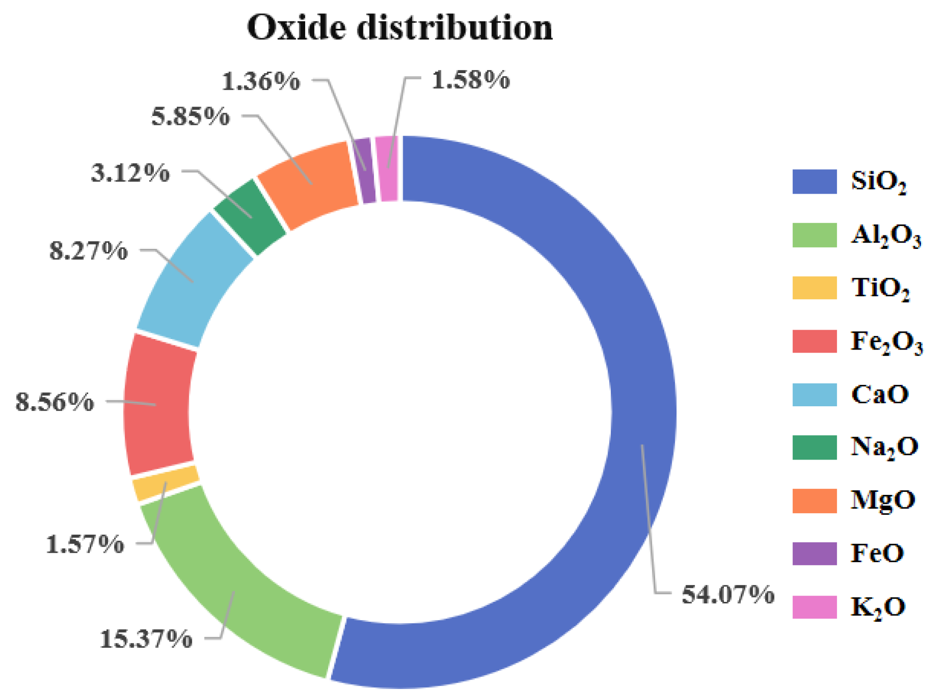
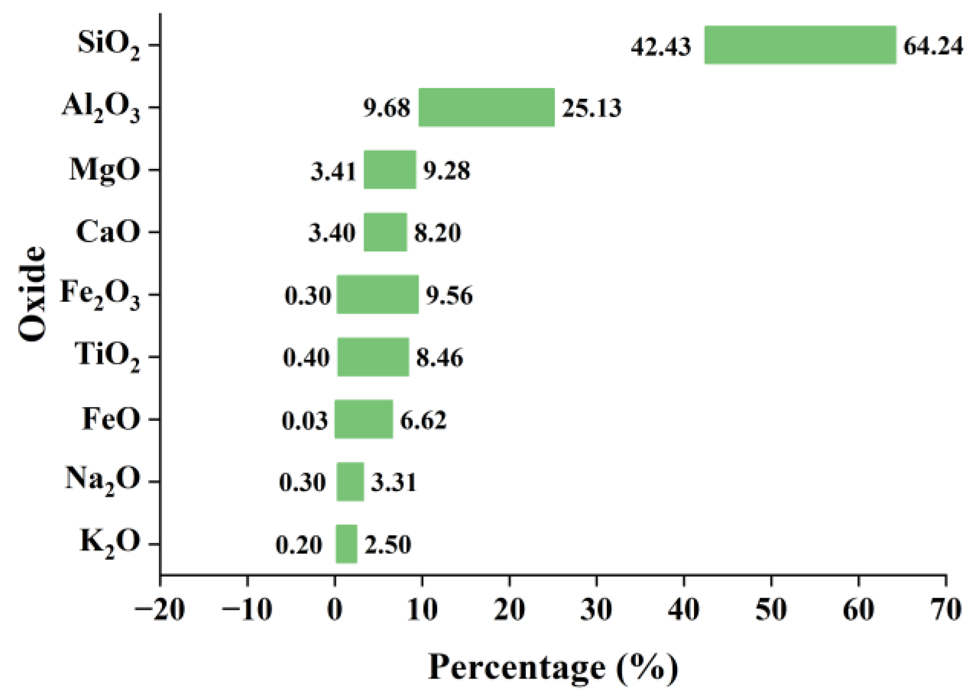
3.1. Description of Variables and Correlation Analysis

The elastic modulus of basalt fibers is closely correlated to their oxide composition.

Table 1. The range, mean, and variance of the input variables.

Input Variable	Minimum–Maximum	Mean	Standard Deviation
SiO2/wt%	42.43–66.90	54.07	4.54
Al2O3/wt%	8.70–25.60	15.37	3.75
TiO2/wt%	0.00–8.46	1.57	1.31
Fe2O3/wt%	0.30–19.34	8.56	3.65
CaO/wt%	3.20–18.91	8.27	2.26
Na2O/wt%	0.20–14.00	3.12	1.75
MgO/wt%	1.70–19.44	5.85	2.69
FeO/wt%	0.00–6.62	1.36	1.86
K2O/wt%	0.00–9.35	1.58	1.18

summarizes the range, mean, and variance of the input variables (oxides), while Figure 1 presents a pie chart depicting the average percentage of each oxide in the database. Among all oxides, SiO₂ is the most abundant, with content ranging from 42.43% to 66.90% and an average of 54.07%. Following SiO₂, Al₂O₃ shows content ranging from 8.70% to 25.60% and an average of 15.37%. These oxides form the structural backbone of basalt fibers, acting as network formers that provide the fundamental mechanical properties. Other oxides are generally regarded as network modifiers, which alter the network structure of basalt fibers and significantly influence their mechanical behavior.

Table 1 also reveals that SiO₂ and Al₂O₃ exhibit relatively small standard deviations, indicating that the primary components of basalt fiber exhibit minimal fluctuation in content, whereas other oxides have broader distribution ranges. Figure 2 provides a Pearson correlation coefficient (PCC) heatmap illustrating the relationships between each oxide and the elastic modulus. The absolute PCC values for SiO₂-Fe₂O₃, SiO₂-Al₂O₃, and Al₂O₃-CaO are 0.62, 0.51, and 0.43, respectively, while the correlations among other variables remain below 0.40. This indicates a weak correlation among the input variables, which is favorable for constructing a stable machine learning model.

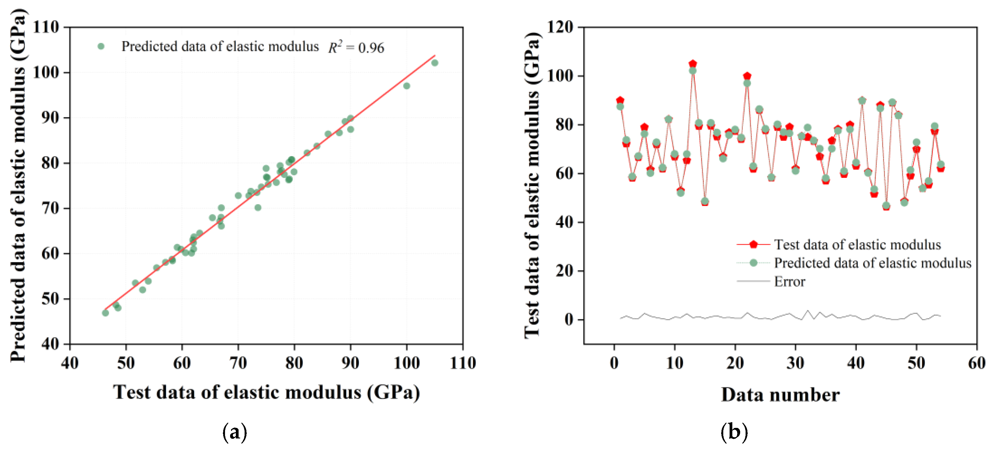
3.2. Model Performance

To obtain the best performance for each model, grid search combined with k-fold cross-validation (k = 5) was employed to determine the optimal combination of model parameters. The coefficient of determination (R²), root-mean-square error (RMSE), and mean absolute error (MAE) were introduced to evaluate the performance of each model in predicting the elastic modulus of basalt fiber. Smaller RMSE and MAE values indicate better predictive accuracy of the model, while an R² value closer to 1 signifies a stronger fit to the test set. The hyper-parameter ranges and optimal parameters for each model are shown in

Table A2. The hyper-parameters ranges and the optimum values.

Model	Hyper-Parameter	Range	Optimum
MLR	-	-	-
KNN	n_neighbors	[1, 50]	22
	weights	[’uniform’, ’distance’]	uniform
	metric	[’euclidean’, ’manhattan’, ’minkowski’]	minkowski
DT	criterion	[’squared_error’, ’friedman_mse’, ’absolute_error’, ’poisson’]	squared_error
	max_depth	[1, 100]	4
	min_samples_split	[2, 20]	2
	min_samples_leaf	[1, 20]	1
	max_features	[None, ’sqrt’, ’log2’]	None
SVR	C	[0.1, 1, 10, 100, 1000]	1.0
	kernel	[’linear’, ’poly’, ’rbf’, ’sigmoid’]	rbf
	gamma	[’scale’, ’auto’]	scale
ANN	hidden_layer_sizes	[(50,50), (100, 100), (100, 50)]	(100, 100)
	activation	[’identity’, ’logistic’, ’tanh’, ’relu’]	relu
	solver	[’lbfgs’, ’sgd’, ’adam’]	adam
	learning_rate	[’constant’, ’invscaling’, ’adaptive’]	constant
	alpha	[0.0001, 0.02, 0.05]	0.02
RF	n_estimators	[10, 300]	141
	max_depth	[1, 100]	12
	min_samples_split	[2, 10]	2
	min_samples_leaf	[1, 10]	1
XGBoost	n_estimators	[50, 500]	86
	learning_rate	[0.01, 0.1, 0.2, 0.3]	0.1
	max_depth	[3, 10]	6
	subsample	[0.5, 1.0]	0.9
	gamma	[0, 10]	0
CatBoost	iterations	[50, 1000]	1000
	learning_rate	[0.01, 0.02, 0.03, 0.04, 0.05, 0.06, 0.07, 0.08, 0.09, 0.1, 0.2, 0.3]	0.03
	depth	[3, 10]	7
	l2_leaf_reg	[1, 10]	3
	bagging_temperature	[0, 1]	1
	random_strength	[1, 10]	1

(Appendix B). The performance of each model is shown in

Table 2. The performance of each model.

Model	Training Data			Test Data
	R2	RMSE	MAE	R2	RMSE	MAE
MLR	0.2951	10.3082	8.0533	0.1703	11.6958	8.7801
KNN	0.5318	8.4015	5.4992	0.4270	9.7199	6.8333
DT	1.0000	0.0407	0.0052	0.0516	12.5045	8.1983
SVR	0.1854	11.0816	8.6477	0.1099	12.1137	9.1008
ANN	0.9856	1.2547	0.3789	0.9209	5.3056	2.5518
RF	0.9184	3.5075	2.3776	0.3916	10.0152	6.4477
XGBoost	1.0000	0.0408	0.0058	0.9390	4.9997	2.2462
CatBoost	0.9993	0.3207	0.2613	0.9554	4.7556	2.0323

and Figure 3.

The R² values of the models DT, ANN, XGBoost, and CatBoost on the training set are nearly 1, accompanied by lower RMSE and MAE values, indicating strong performance during training. On the test set, the CatBoost model achieves an R² of 0.9554, an RMSE of 4.7556, and an MAE of 2.0323, demonstrating the lowest error and the highest degree of fit. Although the R², RMSE, and MAE values of XGBoost are comparable to those of CatBoost, the latter outperforms XGBoost in terms of overall error reduction and predictive accuracy. The ranking of predictive accuracy among the models is as follows: CatBoost, XGBoost, ANN, KNN, RF, MLR, SVR, and DT. CatBoost’s superior performance is attributed to its ability to handle nonlinear relationships, work effectively with small datasets, minimize overfitting, and automatically optimize hyper-parameters. These advantages position it as the best-performing model in this study, surpassing other tree-based algorithms such as RF and DT. Furthermore, the study highlights CatBoost’s strong adaptability to small datasets, further demonstrating its robustness in predictive tasks. Overall, these findings confirm that the CatBoost model delivers the highest predictive accuracy among all models evaluated.

Figure 4a shows a linear regression plot comparing the actual values to the predicted values of the CatBoost model on the test set. Figure 4b illustrates the test set data, predicted values, and corresponding absolute errors. The results reveal strong alignment between the actual and predicted values, with relatively small discrepancies. Specifically, the mean error for the elastic modulus is only 1.19, underscoring the CatBoost model’s accuracy. These findings demonstrate the model’s effectiveness in predicting the elastic modulus of basalt fibers based on their chemical composition.

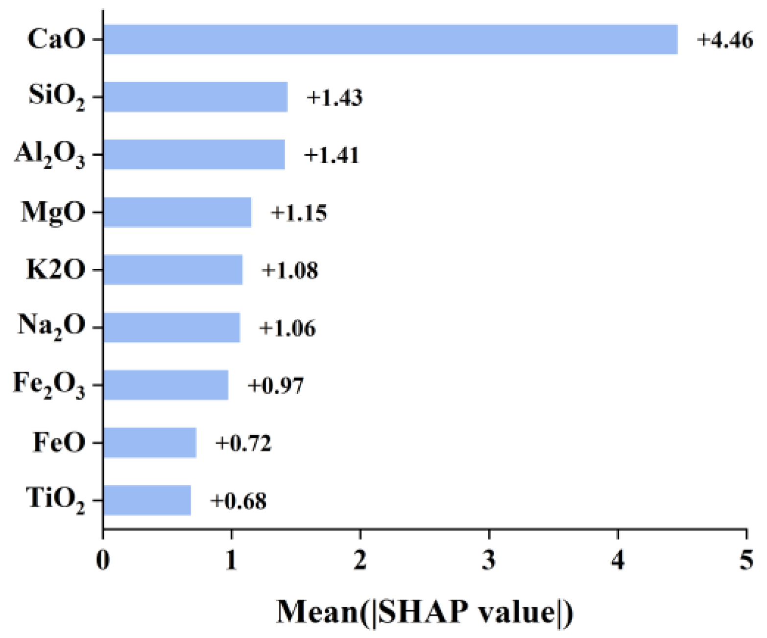
3.3. SHAP Interpretation

The evaluation of model performance demonstrates that the CatBoost model achieves the highest accuracy in the elastic modulus prediction task. However, its complexity poses challenges in understanding and interpreting its behavior during model training, testing, and internal decision-making processes. This lack of interpretability limits the model’s transparency and credibility in practical applications. To address this limitation, this study utilizes the SHAP method to compute the specific contribution (SHAP value) of each input variable to the elastic modulus of basalt. By quantifying the importance of each oxide, SHAP provides consistent, fair, and interpretable insights, enhancing the model’s transparency and practical utility.

Figure 5 demonstrates the importance of each oxide in predicting the elastic modulus, ranked by their average absolute SHAP values. In descending order of importance, the key oxides are CaO, SiO₂, Al₂O₃, MgO, K₂O, Na₂O, Fe₂O₃, FeO, and TiO₂. Notably, CaO has the most pronounced influence on the elastic modulus, a phenomenon not previously observed in previous studies. In the melt state during fiber formation, divalent CaO plays a critical role as a network modifier, significantly enhancing ionic mobility. Meanwhile, Ca²⁺ ions, characterized by their large ionic radius and moderate charge, are effective in balancing basalt network charges [18,52]. Their presence facilitates the incorporation of additional atoms into the fiber structure, forming stable R-O ionic bonds that aggregate the network structure and enhance the elastic modulus. SiO₂ and Al₂O₃ follow CaO in importance, contributing significantly to the elastic modulus as they form the structural backbone of basalt fibers, endowing them with their fundamental mechanical properties. MgO has a similar role to CaO, yet due to the smaller ionic radius of Mg²⁺, it generates a higher electric field intensity. This characteristic promotes the polymerization of polyhedral structures disrupted by alkali metals in the glass network, further improving the fiber’s elastic modulus. The SHAP values for K₂O, Na₂O, and Fe₂O₃ are comparable, reflecting their similar influence on the elastic modulus. Similarly, FeO and TiO₂ exhibit the lowest SHAP values, indicating their minimal impact, likely due to their relatively low concentrations in the dataset. It is noteworthy that the SHAP values for SiO₂, Al₂O₃, MgO, K₂O, Na₂O, Fe₂O₃, FeO, and TiO₂ are only 1/7 to 1/3 of that for CaO. This underscores the role of CaO as a network modifier, significantly enhancing network polymerization and thereby improving the fiber’s elastic modulus. Thus, optimizing the CaO percentage emerges as a critical strategy for enhancing the elastic modulus of basalt fibers.

Pearson correlation analysis reveals that the input variables exhibit relatively weak intercorrelations. Consequently, univariate dependency analysis is employed to visualize the impact of individual variables on the machine learning model’s prediction results. Figure 6 illustrates the relationship between the oxide and the elastic modulus, where the x-axis represents the input variable values and the y-axis represents the SHAP values. This figure effectively highlights whether a specific oxide has a positive or negative influence on the elastic modulus prediction. For instance, in the case of CaO, when the SHAP value exceeds 0, the corresponding range of CaO content is [3.40, 8.20]. Within this range, the predicted elastic modulus of basalt fibers increases. Figure 7 summarizes the positive contributions of each input variable to the predicted elastic modulus of basalt fibers.

4. Conclusions

This study constructed eight machine learning prediction models, namely MLR, KNN, DT, SVR, ANN, RF, XGBoost, and CatBoost, to assess the elastic modulus of basalt fiber based on oxide composition. SHAP analysis was conducted to examine the relevance and interaction of oxide composition on the elastic modulus. The following are the main conclusions.

(1)

The correlation among the oxide variables is weak, and there is no significant linear correlation with the elastic modulus.

(2)

The CatBoost model performed best for elastic modulus prediction, scoring 0.9554, 4.7556, and 2.0323 of R², RMSE, and MAE, respectively.

(3)

The SHAP results revealed a ranking of the input variable importance for the XGBR model of, in descending order, CaO > SiO₂ > Al₂O₃ > MgO > K₂O > Na₂O > Fe₂O₃ > FeO > TiO₂.

(4)

The calcium oxide content has a significant impact on the elastic modulus of basalt fibers, indicating that adjusting the calcium oxide content is an important approach to improving the elastic modulus of basalt fibers.

References

1. Dhand, V.; Mittal, G.; Rhee, K.Y.; Park, S.J.; Hui, D. A short review on basalt fiber reinforced polymer composites. Compos. B Eng. 2015, 73, 166–180. [Google Scholar] [CrossRef]
2. Ivanitskii, S.G.; Gorbachev, G.F. Continuous basalt fibers: Production aspects and simulation of forming processes. I. State of the art in continuous basalt fiber technologies. Powder Metall. Met. Ceram. 2011, 50, 125. [Google Scholar] [CrossRef]
3. Shi, F.J. A study on structure and properties of basalt fiber. Appl. Mech. Mater. 2012, 238, 17–21. [Google Scholar]
4. Antunes, P.; Domingues, F.; Granada, M.; André, P. Mechanical Properties of Optical Fibers; INTECH Open Access Publisher: London, UK, 2012. [Google Scholar]
5. Li, G.; Chen, Y.; Wei, G. Continuous fiber reinforced meta-composites with tailorable Poisson’s ratio and effective elastic modulus: Design and experiment. Compos. Struct. 2024, 329, 117768. [Google Scholar]
6. Bi, C.; Tang, G.H.; He, C.B.; Yang, X.; Lu, Y. Elastic modulus prediction based on thermal conductivity for silica aerogels and fiber reinforced composites. Ceram. Int. 2022, 48, 6691–6697. [Google Scholar]
7. Alshahrani, A.; Kulasegaram, S.; Kundu, A. Elastic modulus of self-compacting fibre reinforced concrete: Experimental approach and multi-scale simulation. Case Stud. Constr. Mater. 2023, 18, e01723. [Google Scholar] [CrossRef]
8. Wang, Y.; Hu, S.; Sun, X. Experimental investigation on the elastic modulus and fracture properties of basalt fiber-reinforced fly ash geopolymer concrete. Constr. Build. Mater. 2022, 338, 127570. [Google Scholar] [CrossRef]
9. Asadi, A.; Baaij, F.; Mainka, H.; Rademacher, M.; Thompson, J.; Kalaitzidou, K. Basalt fibers as a sustainable and cost-effective alternative to glass fibers in sheet molding compound (SMC). Compos. B Eng. 2017, 123, 210–218. [Google Scholar]
10. Jagadeesh, P.; Rangappa, S.M.; Siengchin, S. Basalt fibers: An environmentally acceptable and sustainable green material for polymer composites. Constr. Build. Mater. 2024, 436, 136834. [Google Scholar]
11. Khandelwal, S.; Rhee, K.Y. Recent advances in basalt-fiber-reinforced composites: Tailoring the fiber-matrix interface. Compos. B Eng. 2020, 192, 108011. [Google Scholar]
12. Guo, Z.S.; Hao, N.; Wang, L.M.; Chen, J.X. Review of Basalt-Fiber-Reinforced Cement-based Composites in China: Their Dynamic Mechanical Properties and Durability. Mech. Compos. Mater. 2019, 55, 107–120. [Google Scholar] [CrossRef]
13. Tumadhir, M. Borhan Thermal and mechanical properties of basalt fibre reinforced concrete. Int. J. Civ. Environ. Eng. 2013, 7, 334–337. [Google Scholar]
14. Wang, D.; Ju, Y.; Shen, H.; Xu, L. Mechanical properties of high performance concrete reinforced with basalt fiber and polypropylene fiber. Constr. Build. Mater. 2019, 197, 464–473. [Google Scholar]
15. Lopresto, V.; Leone, C.; De Iorio, I. Mechanical characterisation of basalt fibre reinforced plastic. Compos. B Eng. 2011, 42, 717–723. [Google Scholar]
16. Ding, L.; Liu, Y.; Liu, J.; Wang, X. Correlation analysis of tensile strength and chemical composition of basalt fiber roving. Polym. Compos. 2019, 40, 2959–2966. [Google Scholar] [CrossRef]
17. Deák, T.; Czigány, T. Chemical Composition and Mechanical Properties of Basalt and Glass Fibers: A Comparison. Text. Res. J. 2009, 79, 645–651. [Google Scholar]
18. Wu, Z.; Liu, J.; Chen, X. Continuous Basalt Fiber Technology; Chemical Industry Press Co., Ltd.: Beijing, China, 2020; p. 238. [Google Scholar]
19. Wei, C.; Zhou, Q.; Deng, K.; Lin, Y.; Wang, L.; Luo, Y.; Zhang, Y.; Zhou, H. Alkali resistance prediction and degradation mechanism of basalt fiber: Integrated with artificial neural network machine learning model. J. Build. Eng. 2024, 86, 108850. [Google Scholar]
20. Sun, Z.; Li, Y.; Yang, Y.; Su, L.; Xie, S. Splitting tensile strength of basalt fiber reinforced coral aggregate concrete: Optimized XGBoost models and experimental validation. Constr. Build. Mater. 2024, 416, 135133. [Google Scholar]
21. Alarfaj, M.; Qureshi, H.J.; Shahab, M.Z.; Javed, M.F.; Arifuzzaman, M.; Gamil, Y. Machine learning based prediction models for spilt tensile strength of fiber reinforced recycled aggregate concrete. Case Stud. Constr. Mater. 2024, 20, e02836. [Google Scholar]
22. Machello, C.; Bazli, M.; Rajabipour, A.; Rad, H.M.; Arashpour, M.; Hadigheh, A. Using machine learning to predict the long-term performance of fibre-reinforced polymer structures: A state-of-the-art review. Constr. Build. Mater. 2023, 408, 133692. [Google Scholar] [CrossRef]
23. Eduard, K.; Rainer, G.; Jona, S. Basalt, glass and carbon fibers and their fiber reinforced polymer composites under thermal and mechanical load. AIMS Mater. Sci. 2016, 3, 1561–1576. [Google Scholar]
24. Wei, B.; Cao, H.; Song, S. Tensile behavior contrast of basalt and glass fibers after chemical treatment. Mater. Des. 2010, 31, 4244–4250. [Google Scholar] [CrossRef]
25. Sergey, I.G.; Evgeniya, S.Z.; Sergey, S.P.; Bogdan, I.L. Correlation of the chemical composition, structure and mechanical properties of basalt continuous fibers. AIMS Mater. Sci. 2019, 6, 806–820. [Google Scholar]
26. Wang, L. Study on Effect of Basalt Fiber Component on Elastic Modulus. Master of Thesis, Southeast University, Nanjing, China, 2021. [Google Scholar]
27. Kuzmin, K.L.; Gutnikov, S.I.; Zhukovskaya, E.S.; Lazoryak, B.I. Basaltic glass fibers with advanced mechanical properties. J. Non-Cryst. Solids 2017, 476, 144–150. [Google Scholar] [CrossRef]
28. Manylov, M.S.; Gutnikov, S.I.; Lipatov, Y.V.; Malakho, A.P.; Lazoryak, B.I. Effect of deferrization on continuous basalt fiber properties. Mendeleev Commun. 2015, 25, 386–388. [Google Scholar] [CrossRef]
29. Kuzmin, K.L.; Zhukovskaya, E.S.; Gutnikov, S.I.; Pavlov, Y.V.; Lazoryak, B.I. Effects of Ion Exchange on the Mechanical Properties of Basaltic Glass Fibers. Int. J. Appl. Glass Sci. 2016, 7, 118–127. [Google Scholar] [CrossRef]
30. Wu, Z.; Liu, J.; Jiang, M.; Wang, Y.; Lei, L. A High-Temperature Resistant Basalt Fiber Composition. China Patent CN 201410139342.1, 6 January 2016. [Google Scholar]
31. Wei, B. Evaluation of Basalt Fiber and Its Hybrid Reinforced Composite Performance. Master’ Thesis, Harbin Institute of Technology, Harbin, China, 2008. [Google Scholar]
32. Wang, X.; Sun, K.; Shao, J.; Ma, J. Fracture properties of graded basalt fiber reinforced concrete: Experimental study and Mori-Tanaka method application. Constr. Build. Mater. 2023, 398, 132510. [Google Scholar] [CrossRef]
33. Ramachandran, B.E.; Velpari, V.; Balasubramanian, N. Chemical durability studies on basalt fibres. J. Mater. Sci. 1981, 16, 3393–3397. [Google Scholar] [CrossRef]
34. Dong, J.F.; Wang, Q.Y.; Guan, Z.W.; Chai, H.K. High-temperature behaviour of basalt fibre reinforced concrete made with recycled aggregates from earthquake waste. J. Build. Eng. 2022, 48, 103895. [Google Scholar] [CrossRef]
35. Xing, D.; Chang, C.; Xi, X.Y.; Hao, B.; Zheng, Q.; Gutnikov, S.I.; Lazoryak, B.I.; Ma, P.C. Morphologies and mechanical properties of basalt fibre processed at elevated temperature. J. Non-Cryst. Solids 2022, 582, 121439. [Google Scholar] [CrossRef]
36. Nasir, V.; Karimipour, H.; Taheri-Behrooz, F.; Shokrieh, M.M. Corrosion behaviour and crack formation mechanism of basalt fibre in sulphuric acid. Corros. Sci. 2012, 64, 1–7. [Google Scholar]
37. Li, R.; Gu, Y.; Zhang, G.; Yang, Z.; Li, M.; Zhang, Z. Radiation shielding property of structural polymer composite: Continuous basalt fiber reinforced epoxy matrix composite containing erbium oxide. Compos. Sci. Technol. 2017, 143, 67–74. [Google Scholar]
38. Ahmad, M.R.; Chen, B. Effect of silica fume and basalt fiber on the mechanical properties and microstructure of magnesium phosphate cement (MPC) mortar. Constr. Build. Mater. 2018, 190, 466–478. [Google Scholar]
39. Vejmelková, E.; Koňáková, D.; Scheinherrová, L.; Doleželová, M.; Keppert, M.; Černý, R. High temperature durability of fiber reinforced high alumina cement composites. Constr. Build. Mater. 2018, 162, 881–891. [Google Scholar] [CrossRef]
40. Qin, J.; Qian, J.; Li, Z.; You, C.; Dai, X.; Yue, Y.; Fan, Y. Mechanical properties of basalt fiber reinforced magnesium phosphate cement composites. Constr. Build. Mater. 2018, 188, 946–955. [Google Scholar] [CrossRef]
41. Tang, C.; Jiang, H.; Zhang, X.; Li, G.; Cui, J. Corrosion Behavior and Mechanism of Basalt Fibers in Sodium Hydroxide Solution. Materials 2018, 11, 1381. [Google Scholar] [CrossRef]
42. Li, M.; Gong, F.; Wu, Z. Study on mechanical properties of alkali-resistant basalt fiber reinforced concrete. Constr. Build. Mater. 2020, 245, 118424. [Google Scholar] [CrossRef]
43. ISO 9163:2005(E); Textile Glass—Rovings—Manufacture of Test Specimens and Determination of Tensile Strength of Impregnated Rovings. International Organization Standardization: Brussels, Belgium, 2005.
44. ISO/DIS 5079(en); Textile Fibres—Determination of Breaking Force and Elongation at Break of Individual Fibres. International Organization Standardization: Brussels, Belgium, 1999.
45. DIN 65382; Aerospace; Reinforcement Fibres for Plastics; Tensile Test of Impregnated Yarn Test Specimens. German Institute for Standardisation: Berlin, Germany, 1988.
46. GB/T 7690.1−2001; Reinforcements—Test Method for Yarns—Part 1: Determination of Linear Density. Standardization Administration of China: Beijing, China, 2001.
47. GB/T 38897−2020; Non-Destructive Testing—Measurement Method for Material Elastic Modulus and Poisson’s Ratio Using Ultrasoinc Velocity. Standardization Administration of China: Beijing, China, 2020.
48. GB/T 3362−2017; Test Methods for Tensile Properties of Carbon Fiber Multifilament. Standardization Administration of China: Beijing, China, 2017.
49. ASTM, C1557−14; Standard Test Method for Tensile Strength and Young’s Modulus of Fibers. American Society Testing and Materials: West Conshohocken, PA, USA, 2014.
50. ASTM, D3379-75; Standard Test Method for Tensile Strength and Young’s Modulus for High-Modulus Single-Filament Materials. American Society Testing and Materials: West Conshohocken, PA, USA, 1989.
51. Lundberg, S.M.; Lee, S.I. A unified approach to interpreting model predictions. In Proceedings of the 31st International Conference on Neural Information Processing Systems, Long Beach, CA, USA, 4–9 December 2017; Curran Associates Inc.: Red Hook, NY, USA, 2017; pp. 4768–4777. [Google Scholar]
52. Cao, H.; Yan, Y.; Yue, L.; Zhao, J. Basalt Fiber; National Defense Industry Press: Beijing, China, 2017; p. 188. [Google Scholar]
Figure 1. Pie chart of average oxide percentage.
Minerals 15 00387 g001
Figure 2. Pearson correlation coefficient heatmap of variables.
Minerals 15 00387 g002
Figure 3. Performance of each model in training data and test data.
Minerals 15 00387 g003
Figure 4. Comparison of predicated data and test data. (a) Linear regression plot comparing the actual values to the predicted values of the CatBoost model on the test set. (b) The test set data, predicted values, and the corresponding absolute errors.
Minerals 15 00387 g004
Figure 5. Feature importance of input variables.
Minerals 15 00387 g005
Figure 6. Dependence plot of input variables.
Minerals 15 00387 g006
Figure 7. The ranges within which the input variables positively contribute to the TS.
Minerals 15 00387 g007