Article

Correlation and Knowledge-Based Joint Feature Selection for Copper Flotation Backbone Process Design

1
College of Electrical Engineering and Automation, Shandong University of Science and Technology, Qingdao 266590, China
2
College of Information Science and Engineering, Northeastern University, Shenyang 110004, China
*
Author to whom correspondence should be addressed.
Minerals 2025, 15(4), 353; https://doi.org/10.3390/min15040353
Submission received: 17 February 2025 / Revised: 21 March 2025 / Accepted: 24 March 2025 / Published: 27 March 2025

Abstract

:
The intelligentization of flotation design plays a crucial role in enhancing industrial competitiveness and resource efficiency. Our previous work established a mapping relationship between the flotation backbone process graph and label vectors, enabling an intelligent design of the copper flotation backbone process through multilabel classification. Due to the insufficient quantity of training samples in historical databases, traditional feature selection methods perform poorly, owing to insufficient learning. To address the label-specific feature selection problem for this design, this study proposes correlation and knowledge-based joint feature selection (CK-JFS). In this proposed method, label correlations ensure that features specific to strongly related labels are prioritized, while domain knowledge further refines the selection process by applying specialized knowledge to copper flotation. This mode of data and knowledge integration significantly reduces the reliance of label-specific feature selection on the number of training samples. The results demonstrate that CK-JFS achieves significantly higher accuracy and computational efficiency compared to traditional multilabel feature selection algorithms in the context of copper flotation backbone process design.

1. Introduction

Copper flotation plays a vital role in mineral processing and has long been a key focus of academic research [1,2]. Our previous study [3,4] mentioned that copper flotation backbone process design refers to training a multilabel classifier using a copper flotation history database such that the classifier can convert the input features of a new copper flotation sample into a prediction label vector. The prediction label vector can be transformed into a flotation backbone process diagram. The offline modeling and online application process of the intelligent design system are shown in Figure 1. A multilabel classifier usually suffers from “the curse of dimensionality”, which increases computational costs and model complexity [5]. Feature selection is an effective tool for preventing overfitting and improving the accuracy of model performance [6,7,8,9,10]. The input features of a new copper flotation sample were obtained by detecting the natural properties of copper ore. Thus, screening unnecessary features can save human labor and financial resources consumed in the detection process. This study filters the original features before training the multilabel model, which is highlighted in the blue box in Figure 1.
Previously, multilabel feature selection has primarily selected the common feature space shared by all sublabels [11,12,13,14,15], but the discriminative features are different for each label. Therefore, label-specific features have been proposed. Label-specific feature selection refers to learning discriminative features relative to each label from the original features. The objective function of efficient and robust feature selection introduces the L21 norm based on the loss function to guide feature sparsity and realize the selection (ERFS) [16] of label-specific features. Studies [17,18,19] have reported that exploiting label correlation can improve multilabel classifier performances, such as learning label-specific features (LLSF) [20] and joint feature selection and classification (JFSC) [21]. By incorporating a feature-sharing function into the objective function of a linear classifier, LLSF prevents two weakly correlated labels from sharing similar label-specific features. JFSC introduces the Fisher discriminant method based on LLSF to realize a large inter-class distance between positive and negative examples and a small inner-class distance between positive and negative examples. However, the label correlation functions of LLSF and JFSC cannot punish the condition in which the label-specific features of two strongly correlated labels are dissimilar. Furthermore, current multilabel feature selection algorithms cannot use domain knowledge. In the design of the copper flotation process, although there is a certain accumulation of domain knowledge, it is not exhaustive, and the number of historical database cases is limited. The combination of data and knowledge is expected to overcome the difficulty of “insufficient learning” and significantly improve the effect of label-specific feature selection.
In response to the deficiencies of the existing methods described above, the novel contributions of this paper are as follows: (1) the proposed CK-JFS utilizes the label correlation of training set samples through a correlation-based function, which renders the label-specific features of two strongly correlated labels similar; (2) the proposed CK-JFS fully utilizes domain knowledge. The knowledge-based function makes the label-specific features conform to the domain knowledge.
The remainder of this paper is organized as follows: In Section 2, we introduce the application background and theoretical basis of the proposed CK-JFS. In Section 3, we elaborate on the objective function and optimization method of the proposed CK-JFS. In Section 4, empirical evaluations are presented to demonstrate the superiority of the proposed CK-JFS by comparing it with benchmark multilabel feature selection algorithms. Finally, the conclusions are presented in Section 5.

2. Preliminaries

2.1. Notations

The original features are all detected as natural properties of copper ores in historical copper flotation samples. Suppose that N samples and M original features are present. Denote the feature matrix as X = [x1:, x2:, …, xN:]T R N×M, where xn: = [Xn1, Xn2, …, XnM] ∈ R M is the feature vector of sample n. In the design of the copper flotation backbone process as a multilabel problem, each copper flotation sample can be assigned with multiple sublabels simultaneously [22,23]. Let Y = [y1:, y2:, …, yN:]T ∈ {−1,1}N×K be the label matrix, where K is the label number, and yn: = [Yn1, Yn2, …, YnK] ∈ {−1,1}1×K is the label vector of sample n. Ynk is the value of sample n at label k. If the sample n is positive at the label k, Ynk = 1; otherwise, Ynk = −1. Our purpose with the proposed CK-JFS is to optimize the coefficient matrix W = [w:1, w:2, …, w:K] ∈ R M×K, where w:k = [W1k, W2k, …, WMk] ∈ R 1 is the coefficient vector of label k, and Wmk is the coefficient of feature m to label k. A larger absolute value of Wmk means that the feature m is more important for the label k.
The historical database of N = 228 copper flotation samples was provided by a certain research institute. The samples have M = 85 original features and K = 15 sublabels.

2.2. Sublabels

Three tasks must be completed in the design: the product scheme, the flotation scheme, and the grinding scheme. The product scheme includes four sublabels, which indicate the presence of molybdenum, lead, zinc, and sulfur concentrates in the product. The flotation scheme includes six sublabels, which indicate whether copper requires asynchronous flotation and whether molybdenum, lead, zinc, sulfur, and copper require mixed flotation. The grinding scheme includes five sublabels, which indicate whether the grinding stage of molybdenum is more than two and whether the grinding stages of lead, zinc, sulfur, and copper exceed one. As aforementioned, the three tasks contain 15 sublabels [4]. Because each sublabel is a binary classification problem, samples that do not belong to a positive class are considered negative classes.

2.3. Original Features

Eighty-five original features are listed in Table 1. These features include chemical composition, phase analysis, ore content, gangue content, symbiosis relationship, and particle size. Among these, the symbiotic relationship is not a numerical feature that must be converted into numerical features. Thus, we used 0 to denote the symbiosis between the ore and gangue and 1 to denote that between the ore and other ores.

3. Proposed Approach

3.1. Objective Function

Aiming at local correlation and domain knowledge sensitivity, we optimize W such that the objective function, as shown in Equation (1), is minimized, where λ1, λ2, λ3, and λ4 are hyperparameters. The larger the W m k is, the more important feature m is to label k.
O b j ( W ) = 1 2 L ( W ) + λ 1 W 1 + λ 2 2 F ( W ) + λ 3 4 Ψ ( W ) + λ 4 Φ ( W )

3.1.1. Non-Unique Terms

The first three items in Equation (1) are consistent with JFSC. The least-square loss has been widely used as a loss function, which can be illustrated as X W Y F 2 , where F denotes the Frobenius norm of the matrix. W 1 is employed to model the sparsity of label-specific features, where 1 denotes the L1 norm of the matrix. The Fisher discriminant F(W) is used to maximize the inter-class distances and minimize the intra-class distance. Suppose that P k = x n : Y n k = 1 is a positive set and N k = x n : Y n k = 1 is a negative set. x ¯ k + = [ x ¯ k 1 + , x ¯ k 2 + , , x ¯ k M + ] and x ¯ k = [ x ¯ k 1 , x ¯ k 2 , , x ¯ k M ] are the mean vectors of positive and negative sets in the original feature space, where x ¯ k m + = 1 P k x n : P k X n m and x ¯ k m = 1 N k x n : N k X n m . S k + 2 = w : k T d i a g ( s k + ) w : k and S k 2 = w : k T d i a g ( s k ) w : k are the intra-class distance of positive samples and negative samples, respectively, where s k + and s k are calculated via Equations (2) and (3). S k 2 = w : k T d i a g ( s k ) w : k is the inter-class distance between positive and negative samples, where s k is calculated using Equation (4).
s k + = x n : P k ( x n : x ¯ k + ) ( x n : x ¯ k + )
s k = x n : N k ( x n : x ¯ k ) ( x n : x ¯ k )
s k = ( x ¯ k + x ¯ k ) ( x ¯ k + x ¯ k )
The derivative of L(W) with respect to W can be calculated using Equation (5), and the derivative of F(W) with respect to W can be calculated using Equation (6), where C ∈ R M×K with column vector c:k is defined in Equation (7).
L ( W ) W = 2 ( X T X W X T Y )
F ( W ) W = 2 C W
c : k = s k + + r k s k P k s k

3.1.2. Unique Terms

The last two terms of Equation (1) are unique to the proposed CK-JFS. For machine learning with small samples, weak label correlation often originates from noise and is not worth utilizing. The correlation-based function Ψ ( W ) is used to replace the correlation-based function in JFSC because the proposed Ψ ( W ) uses strong correlation, while the latter uses strong correlation. In addition, the knowledge-based function Φ ( W ) is introduced into the objective function to fully utilize the domain knowledge.

3.2. Correlation-Based Function

To render the prediction of two strongly positively correlated labels consistent to the extent possible, and the prediction of two strongly negatively correlated labels opposite to the extent possible, the correlation-based function is introduced.
To filter out weak label correlations, a correlation threshold, θ, is employed as a hyperparameter. Set a prediction matrix, F = XW. Set a diagonal matrix, A(1) ∈ R K×K, with element A(1)kk defined as Equation (8), where Cor(k, k’) is the Pearson correlation coefficient between labels k and k’, as shown in Equation (9).
A ( 1 ) k k = C o r ( k , k ) k k and C o r ( k , k ) > θ C o r ( k , k ) k k and C o r ( k , k ) < θ 0 otherwise
C o r ( k , k ) = C o r ( k , k ) = n = 1 N ( Y n k y : k ¯ ) ( Y n k y : k ¯ ) n = 1 N ( Y n k y : k ¯ ) 2 n = 1 N ( Y n k y : k ¯ ) 2
When Cor(k, k’) > θ, labels k and k’ are regarded as positively correlated, their corresponding prediction vectors f:k and f:k are similar, and the value of FnkFnk is expected to be close to 0; when Cor(k’, k) < −θ, labels k and k’ are regarded as negatively correlated, their corresponding prediction vectors, f:k and f:k, are opposite, and the value of Fnk + Fnk is expected to be close to 0. Therefore, the correlation-based function Ψ ( W ) can be formulated as Equations (10)–(12), where the diagonal matrix A(2) ∈ R K×K with element A(2)kk is defined via Equation (12).
Ψ ( W ) = k , k = 1 K ψ k k ( W )
ψ k k ( W ) = A ( 1 ) k k f : k + A ( 2 ) k k f : k 2 2
A ( 2 ) k k = 1 C o r ( k , k ) θ 1 otherwise
The correlation-based function can be revised as Equation (13), where the diagonal matrix D(A1) R K×K with element D(A1)kk is defined as Equation (14), where the diagonal matrix A ( 3 ) = A ( 1 ) A ( 2 ) .
Ψ ( W ) = k , k = 1 K ψ k k ( W ) = k , k = 1 K A ( 1 ) k k f : k + A ( 2 ) k k f : k F 2 = k , k = 1 K A ( 1 ) k k ( f : k + A ( 2 ) k k f : k ) T ( f : k + A ( 2 ) k k f : k ) = k , k = 1 K A ( 1 ) k k ( f : k T f : k + A ( 2 ) k k f : k T f : k + A ( 2 ) k k f : k T f : k + ( A ( 2 ) k k ) 2 f : k T f : k ) = 2 ( k = 1 K f : k T f : k D ( A 1 ) k k + k , k = 1 K A ( 3 ) k k f : k T f : k ) = 2 ( Tr ( F T F D ( A 1 ) ) + Tr ( F T F A ( 3 ) )
D ( A 1 ) k k = k = 1 K A ( 1 ) k k
The derivative of the correlation-based function with respect to the coefficient matrix is calculated according to Equation (15).
Ψ ( W ) W = 2 ( Tr ( F T F D ( A 1 ) ) W + Tr ( F T F A ( 3 ) ) W = 2 ( 2 X T X W D ( A 1 ) + 2 X T X W A ( 3 ) ) = 4 X T X W ( D ( A 1 ) + A ( 3 ) )

3.3. Knowledge-Based Function

Some domain knowledge in copper flotation has been established. For example, if the zinc concentrate is subjected to bulk flotation, the sulfur concentrate is also subjected to bulk flotation. That can be rewritten as k = 9 and k’ = 8. If Yn8 = 1, Fn9 is expected to be close to 1.
The knowledge-based function Φ ( W ) can be formulated as Equations (16) and (17). ωnkk is used to determine whether the condition for the impact of label k’ on label k is satisfied. If the condition is satisfied, ωnkk = 1; otherwise, ωnkk = 0. νnkk(W) is used to measure the gap between the predicted value and domain knowledge.
Φ ( W ) = n = 1 N k , k = 1 K ϕ n k k ( W )
ϕ n k k ( W ) = ω n k k ν n k k ( W )
ωnkk is defined in Equations (18) and (19). The knowledge-based impacts can be divided into the following two situations: (a) when label k’ is a positive class, ωnkk = 1, and otherwise, ωnkk = 0; (b) when label k’ is a negative class, ωnkk = 1, and otherwise, ωnkk = 0. Thus, we set B(1)kk = 1 in situation (1) and set B(1)kk = −1 in situation (2). In example (1), B(1)98 = 1 and ω n 98 = 1 2 ( 1 + Y n 8 ) . Notably, B(1)∈ R K×K with element B(1)kk is defined as Equation (19).
ω n k k = 1 2 ( 1 + B ( 1 ) k k Y n k )
B ( 1 ) k k = 1 situation ( a ) 1 situation ( b )
νnkk(W) is defined by Equations (20) and (21). If the impact renders label k positive, we set B(2)kk = −1 to render Fnk close to 1. If the impact renders label k negative, we set B(2)kk = 1 to make Fnk close to −1. In the example, B(1)98 = −1 and ν n 98 ( W ) = ( 1 F n 9 ) 2 . Notably, B(2) ∈ R K×K with element B(2)kk is defined as Equation (21).
ν n k k ( W ) = ( 1 + B ( 2 ) k k F n k ) 2
B ( 2 ) k k = 1 the   impact   make   label   k   to   be   positive 1 otherwise
The knowledge-based function can be expressed using Equation (22), where the diagonal matrix B ( 3 ) = B ( 1 ) B ( 2 ) .
Φ ( W ) = 1 2 k , k = 1 K ( 1 ( N * 1 ) + B ( 1 ) k k y : k ) T ( ( 1 ( N * 1 ) + B ( 2 ) k k f : k ) ( 1 ( N * 1 ) + B ( 2 ) k k f : k ) ) = 1 2 k , k = 1 K ( 1 ( N * 1 ) + B ( 1 ) k k y : k ) T ( 1 ( N * 1 ) + 2 B ( 2 ) k k f : k + f : k f : k ) = 1 2 k , k = 1 K ( N + 2 B ( 2 ) k k f : k T 1 ( N * 1 ) + 1 ( 1 * N ) ( f : k f : k ) + B ( 1 ) k k y : k T 1 ( N * 1 )   + 2 B ( 3 ) k k f : k T y : k + B ( 1 ) k k y : k T ( f : k f : k ) ) = 1 2 ( N K 2 + Tr ( Y T 1 ( N * K ) B ( 1 ) T ) + 2 Tr ( F T 1 ( N * K ) B ( 2 ) T )   + K Tr ( ( F F ) 1 ( K * N ) ) + 2 Tr ( F T Y B ( 3 ) T ) + Tr ( ( F F ) B ( 1 ) Y T ) )
Set G = 1 ( K * N ) ( F F )   R K×K, and its diagonal element Gkk is calculated using Equation (23). Tr ( G ) W   R M×K with element is calculated using Equation (24). Set a matrix H(1) R M×K, and its row vector h(1)m: R K is defined by Equation (25). Thus, the third term in Equation (22) with respect to the coefficient matrix is obtained using Equation (26).
G k k = n = 1 N F n k 2
( Tr ( G ) W ) m k = k = 1 K G k k W m k = n = 1 N X n m 2 W m k 2 W m k = 2 n = 1 N X n m 2 W m k
h ( 1 ) m : = n = 1 N X n m 2 1 ( 1 * K )
K Tr ( G ) W = 2 K H ( 1 ) W
Set J = B ( 1 ) Y T ( F F )   R K×K, and its diagonal element Jkk is calculated using Equation (27). Tr ( J ) W   R M×K with element is calculated as Equation (28). Set a matrix, H(2) R M×K, and its element is defined as Equation (29). Thus, the fourth term in Equation (22) with respect to the coefficient matrix is obtained using Equation (30).
J k k = n = 1 N k = 1 K B ( 1 ) k k Y n k F n k 2
( Tr ( J ) W ) m k = k = 1 K J k k W m k = n = 1 N k = 1 K B ( 1 ) k k Y n k X n m 2 W m k 2 W m k = 2 n = 1 N k = 1 K B ( 1 ) k k Y n k X n m 2 W m k
H ( 2 ) m k = n = 1 N k = 1 K B ( 1 ) k k Y n k X n m 2
Tr ( J ) W = 2 H ( 2 ) W
The derivative of the knowledge-based function with respect to the coefficient matrix is obtained using Equation (31), and Φ ( W ) W   R M×K.
Φ ( W ) W = Tr ( F T 1 ( N * K ) B ( 2 ) T ) W + Tr ( F T Y B ( 3 ) T ) W + 1 2 ( Tr ( G ) W + Tr ( J ) W ) = X T 1 ( N * K ) B ( 2 ) T + X T Y B ( 3 ) T + ( K H ( 1 ) + H ( 2 ) ) W

3.4. Optimization via Accelerated Proximal Gradient

The objective function is convex but nonsmooth because of the L1 norm. We address this issue using the accelerated proximal gradient method [24], which can be expressed using Equation (32), where g(W) is a smooth part, and h(W) is a non-smooth part. g(W) and h(W) can be defined as Equations (33) and (34), respectively.
min { o b j = g ( W ) + h ( W ) }
g ( W ) = 1 2 L ( W ) + λ 2 2 F ( W ) + λ 3 4 Ψ ( W ) + λ 4 Φ ( W )
h ( W ) = λ 1 W 1
The derivative of the smooth part with respect to the coefficient matrix is obtained using Equation (35), and g ( W )   R M×K.
g ( W ) = 1 2 L ( W ) W + λ 2 2 F ( W ) W + λ 3 4 Ψ ( W ) W + λ 4 Φ ( W ) W = X T X W X T Y + λ 2 C W + λ 3 X T X W ( D ( A 1 ) + A ( 3 ) T )   + λ 4 ( X T 1 ( N × K ) B ( 2 ) T + X T Y B ( 3 ) T + ( K H ( 1 ) + H ( 2 ) W )
The further Lipschitz continuity of the smooth part is proven using Equation (36), where Δ W = W 1 W 2 .
  g ( W 1 ) g ( W 2 ) F 2 = X T X Δ W + λ 2 C Δ W + λ 3 X T X Δ W ( D ( A 1 ) + A ( 3 ) T ) + λ 4 ( K H ( 1 ) + H ( 2 ) ) Δ W ) F 2 Δ W F 2 ( X T X F 2 + λ 2 max { C m k 2 } + λ 3 X T X F 2 D ( A 1 ) + A ( 3 ) T F 2   + λ 4 ( max { K H ( 1 ) m k 2 } + max { H ( 2 ) m k 2 } )
Therefore, the Lipschitz constant Lf is obtained via Equation (37).
L f = X T X F 2 + λ 2 max { C m k 2 } + λ 3 X T X F 2 D ( A 1 ) + A ( 2 ) A ( 3 ) T F 2 + λ 4 ( max { K H ( 1 ) m k 2 } + max { H ( 2 ) m k 2 } )
In the accelerated proximal gradient method, the proximal gradient is iterated as shown in Equations (38) and (39). The proximal operator associated with h(W) = λ 1 W 1 is the soft-thresholding operator as expressed in Equation (40).
W ( t ) = W t + b t 1 1 b t ( W t W t 1 )
W t + 1 = p r o x L f , h ( W ( t ) 1 L f g ( W ( t ) ) )
( p r o x L f , h ( W ) ) m k = W m k λ 1 L f W m k λ 1 L f 0 W m k λ 1 L f W m k + λ 1 L f W m k λ 1 L f
Algorithm 1 provides the optimization process of the proposed CK-JFS.
Algorithm 1 Optimization process of CK-JFS
Input: training set{X, Y}, hyperparameter λ1, λ2, λ3, λ4, θ, η.
Initialization:
t 1
b 0 , b 1 1
W 0 , W 1 ( X T X + η I ) 1 X T Y
calculate the matrix C as Equation (7)
calculate the diagonal matrix A(1) as Equation (8)
calculate the diagonal matrix A(2) as Equation (12)
calculate the diagonal matrix D(A1) as Equation (14)
calculate the matrix B(1) as Equation (19)
calculate the matrix B(2) as Equation (21)
calculate the matrix g ( W ) as Equation (35)
repeat
        update Wt as Equation (39)
         b t + 1 1 + 4 b t 1 2 + 1 2
         t t + 1
until stop criterion reached
W W t
Output: W
In addition to being a multilabel feature selection algorithm, CK-JFS can be used as a multilabel classifier. The trained coefficient matrix W can be used directly for multilabel classification. For a new copper flotation sample, i, if Fik = xi:w:k exceeds the classification threshold of label k, the prediction value Preik = 1; otherwise, Preik = −1.

4. Experiments

Owing to the small number of samples in the copper flotation database, leave-one-out cross-validation was adopted. Each sample in the database was used as the only test sample in turn, and the other samples were used as the training set. The number of training and testing sets was equal to the number of samples in the database. Because the knowledge-based function was set according to the domain knowledge of copper flotation, the experiments used only the copper flotation database.

4.1. Label-Specific Feature Selection

In this section, the area under the curve (AUC), which is the area under the receiver operating characteristic curve (ROC), was employed as the label-specific feature selection metric. The ROC is a probability curve that presents the relationships between the true positive rates and the false positive rate with different classification thresholds. A large AUC implies high classifier performance.
The label-specific features of each label were selected in parallel to Algorithm 1. For label k, W m k represents the importance of feature m to label k. Hence, all elements in the coefficient vector w:k are sorted according to their absolute values, and the features with higher importance are preferred. As the number of features increases, the AUC first increases and then decreases because extremely few features will lead to insufficient useful information, and extremely many features will lead to redundancy. The number with the maximum AUC is considered the optimal feature number of label k, and the corresponding features are considered label-specific features of label k. The results of the different feature numbers for each label are shown in Figure 2. The selection results of the label-specific features are presented in Table 2. The number in the third column represents the serial number m corresponding to the feature, and the front feature is significantly important to the label.
As presented in Table 2, the union of the label-specific features is [1, 2, 3, 4, 5, 7, 8, 9, 11, 12, 13, 14, 16, 17, 20, 21, 22, 23, 24, 25, 26, 27, 28, 29, 36, 37, 42, 43, 45, 46, 55, 56, 57, 59, 60, 63, 66, 69, 72, 74, 75, 77, 78, 81]. The number of union features is 44, 41 less than the number of original features. For a new copper flotation sample, only 44 natural properties must be detected and input into the trained multilabel classifier, reducing manpower and saving financial resources consumed in the detection.

4.2. Benchmark Multilabel Feature Selection Algorithm

To evaluate the feature selection effect of the proposed CK-JFS on the copper flotation backbone flowchart recommendation, we compared it with the following multilabel feature selection algorithms. Except for the F-score, the others are ablation experiments of CK-JFS.
AllFea: the label-specific features of each label are original features without any selection.
F-score [25]: for each label, a high F-score indicates that the feature exhibits a significant difference between positive samples and negative samples and a small difference between positive samples or negative samples.
LLSF [20]: by incorporating label correlations into the objective function of a linear classifier, two weakly correlated labels cannot share similar label-specific features.
JFSC [21]: a Fisher discriminant is introduced based on LLSF to realize a large inter-class distance between positive and negative samples and a small intra-class distance for the positive and negative samples.
C-JFS: The correlation-based function is introduced into the objective function. Unlike CK-JFS, C-JFS has no knowledge-based function.
K-JFS: The knowledge-based function is introduced into the objective function. Unlike CK-JFS, K-JFS has no correlation-based function.

4.3. Experimental Result

The multilabel feature selection algorithm performances of five evaluation metrics are displayed in Table 3, Table 4, Table 5, Table 6 and Table 7, where the columns indicate the different multilabel feature selection algorithms, and the rows indicate the different classifiers and decision tasks. The classifiers include multilabel k-nearest neighbor (MLKNN) [26], multilabel support vector machine (MLSVM) [27], CK-JFS, classification tree (CT) [28], and extreme gradient boosting (XGBoost) [29]. The latter two classifiers are transformed into multilabel classifiers using a classifier chain (CC) [30]. We rank the performance of the algorithms for each metric and highlight the best performance in a bold font.
Using 75 cases (five metrics × five classifiers × three tasks), as presented in Table 3, Table 4, Table 5, Table 6 and Table 7, the following conclusions are drawn.
(1)
AllFea performs best in 1 case and worst in 51 cases. This is because dimension disasters reduce the performance of the classifier, indicating the necessity of feature selection.
(2)
F-score performs best in 1 case and worst in 12 cases. Although the F-score reduces the feature dimensions, it does not use the correlation between labels.
(3)
LLSF, JFSC, and C-JFS perform best in two, five, and eight cases, respectively, because they use label correlations; however, they do not use domain knowledge.
(4)
K-JFS performs best in 17 cases because it uses domain knowledge, but it does not use label correlation.
(5)
The proposed CK-JFS achieves the best performance in 41 cases and is ranked second in 20 cases. This is because the algorithm not only utilizes domain knowledge but also utilizes label correlation. The fusion of data and domain knowledge notably mitigates the reliance on label-specific feature selection on the quantity of training samples, enabling the proposed method to achieve superior performance under small-sample conditions.
(6)
Thus, the proposed CK-JFS outperforms the benchmark multilabel feature selection algorithms.

4.4. Hypothesis Test

The Bonferroni–Dunn test [31] and t-test [32] are used in this paper to analyze the performance of the benchmark algorithms.

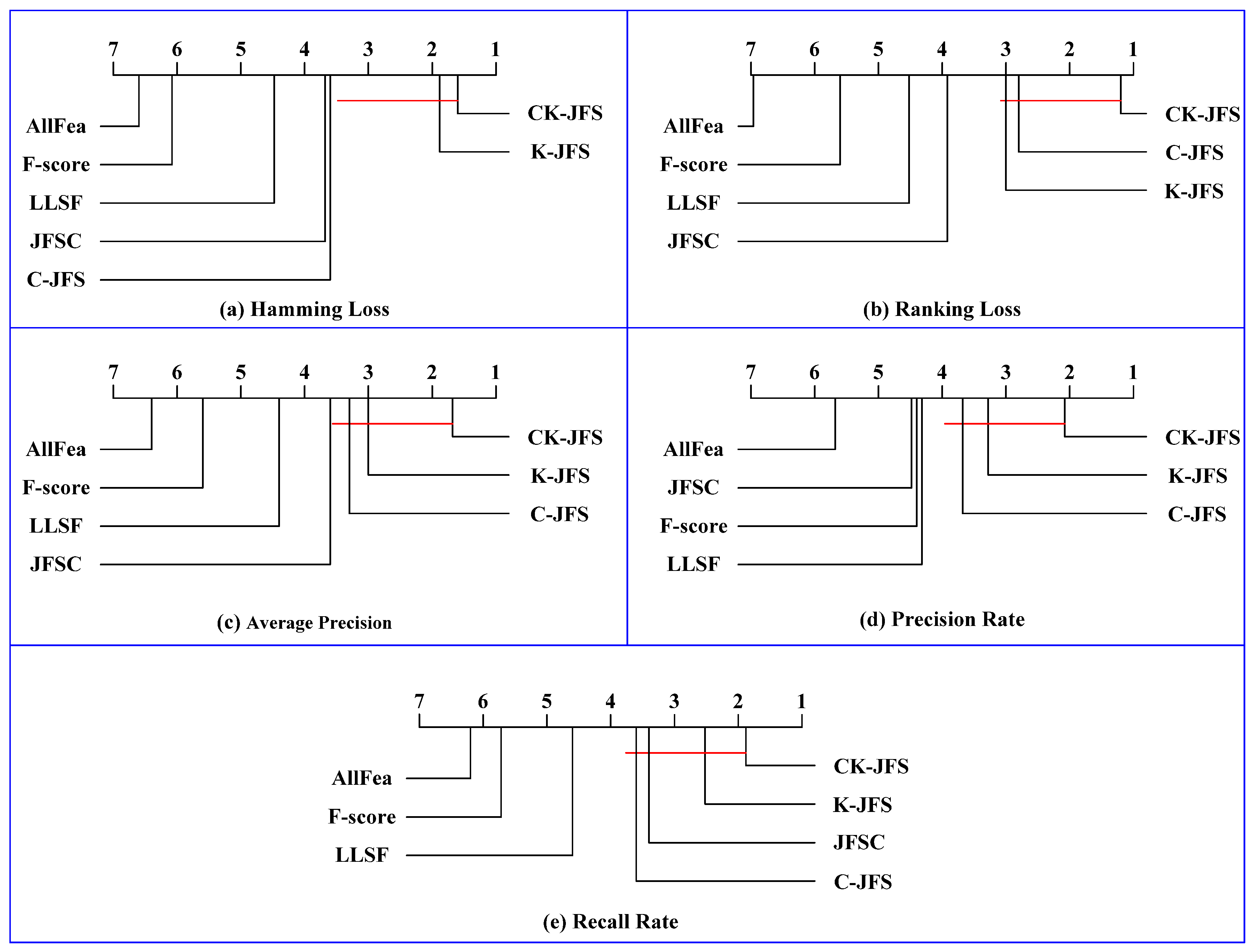
4.4.1. Bonferroni–Dunn Test

To determine the superiority of the proposed CK-JFS, the Bonferroni–Dunn test is executed. The critical distance (CD) is defined by Equation (41). We can obtain qα = 2.394 and CDα = 1.888 at the significance level α = 0.1.
C D α = q α G ( G + 1 ) 6 D
Using the proposed CK-JFS as the control algorithm, the CD diagrams for each metric are obtained, as in Figure 3. In each sub figure, the average ranking of each algorithm is indicated along the axis, and the red line in represents CDα.
Using Figure 1, the following conclusions are drawn:
(1)
The average rankings of the proposed CK-JFS on all metrics are marked on the rightmost side of the axis, indicating that the proposed CK-JFS achieves superior performance over the entire metric to those of the benchmark algorithms.
(2)
CK-JFS achieves statistically superior performance to that of the benchmark algorithms AllFea, F-score, and LLSF.
(3)
CK-XGBoost does not achieve superior performance to that of JFSC in recall rates, but it achieves superior performance to that of JFSC in the other four metrics.
(4)
CK-JFS achieves a superior performance to that of C-JFS in terms of the Hamming loss, but it does not achieve superior performance to that of C-JFS in the other four metrics.
(5)
The statistical differences between CK-JFS and K-JFS cannot be proven for all metrics.

4.4.2. T-Test

A paired t-test was adopted for algorithms that were not proven to be significantly different from CK-JFS in the Bonferroni–Dunn test. The original hypothesis of the paired t-test is that “two algorithms have the equal performance”. We calculated τt using Equation (42), where μ and σ are the mean and the standard deviations, respectively, of the differences in the metrics between the proposed CK-JFS and a benchmark algorithm.
τ t = D μ σ
The results of the paired t-test between the proposed CK-JFS and the benchmark algorithms are present in Table 8, where the blank space indicates that the algorithm has been proven to be significantly different from CK-JFS for the metric in the Bonferroni–Dunn test. Suppose a significance level of α = 0.1. If the p-value < 0.1, the original hypothesis is rejected.
Table 8 indicates that, except for K-JFS with the recall rate (bold significant), the other algorithms are significantly different from CK-JFS.

5. Conclusions

This study has presented a novel approach to addressing the challenge of multilabel feature selection in copper flotation backbone process design. The proposed correlation and knowledge-based joint feature selection (CK-JFS) method integrates two critical components: the correlation-based function that prioritizes features associated with strongly related labels and the knowledge-based function that incorporates domain-specific insights for flotation optimization. The results demonstrate the effectiveness of CK-JFS in enhancing feature selection processes within the context of flotation design.
From a theoretical perspective, the proposed method overcomes the challenge of insufficient learning for small-sample cases. The integration of data and knowledge serves to alleviate the dependence of label-specific feature selection on the volume of training samples. Furthermore, it establishes a novel framework for enhancing the efficacy of small-sample machine learning. From an applied perspective, the proposed method contributes to the broader field of artificial intelligence applications in mineral processing, offering a promising framework for improving operational efficiency and decision-making in complex industrial systems.
However, this study only applies to multilabel classification and not to multilabel regression. Overcoming this limitation will be the subject of our future work.

Author Contributions

Conceptualization, F.W.; methodology, F.W.; software, H.D.; validation, H.D.; formal analysis, H.D.; investigation, F.W.; resources, D.H.; data curation, D.H.; writing—original draft preparation, H.D.; writing—review and editing, H.D.; visualization, F.W.; supervision, Y.L.; project administration, D.H.; funding acquisition, Y.L. All authors have read and agreed to the published version of the manuscript.

Funding

This work was supported by the Key Technologies Research and Development Program of China (2021YFF0602404; 2021YFC2902703), the National Natural Science Foundation of China (Grant No. 62073060; 61973057; 62173078), and the Innovative Research Group Project of the National Natural Science Foundation of China (Grant No. 61621004), for which the authors express their appreciation.

Data Availability Statement

The original contributions presented in this study are included in the article. Further inquiries can be directed to the corresponding author.

Conflicts of Interest

The authors declare no conflict of interest.

References

  1. Feng, Q.; Zhang, Y.; Zhang, G.; Han, G.; Zhao, W. A novel sulfidization system for enhancing hemimorphite flotation through Cu/Pb binary metal ions. Int. J. Min. Sci. Technol. 2024, 34, 1741–1752. [Google Scholar] [CrossRef]
  2. Shen, Q.; Wen, S.; Hao, J.; Feng, Q. Flotation separation of chalcopyrite from pyrite using mineral fulvic acid as selective depressant under weakly alkaline conditions. Trans. Nonferrous Met. Soc. China 2025, 35, 313–325. [Google Scholar] [CrossRef]
  3. Dong, H.; Wang, F.; He, D.; Liu, Y. The intelligent decision-making of copper flotation backbone process based on CK-XGBoost. Knowl.-Based Syst. 2022, 243, 108429. [Google Scholar] [CrossRef]
  4. Dong, H.; Wang, F.; He, D.; Liu, Y. Decision system for copper flotation backbone process. Eng. Appl. Artif. Intell. 2023, 123, 106410. [Google Scholar] [CrossRef]
  5. Siblini, W.; Kuntz, P.; Meyer, F. A Review on Dimensionality Reduction for Multi-label Classification. IEEE Trans. Knowl. Data Eng. 2019, 33, 839–857. [Google Scholar] [CrossRef]
  6. Dong, H.; Sun, J.; Sun, X.; Ding, R. A many-objective feature selection for multi-label classification. Knowl.-Based Syst. 2020, 208, 106456. [Google Scholar] [CrossRef]
  7. Liu, J.; Li, Y.; Weng, W.; Zhang, J.; Chen, B.; Wu, S. Feature selection for multi-label learning with streaming label. Neurocomputing 2020, 387, 268–278. [Google Scholar] [CrossRef]
  8. Liu, J.; Lin, Y.; Li, Y.; Weng, W.; Wu, S. Online multi-label streaming feature selection based on neighborhood rough set. Pattern Recognit. 2018, 84, 273–287. [Google Scholar] [CrossRef]
  9. Huang, J.; Li, G.; Huang, Q.; Wu, X. Learning label specific Features and Class-Dependent Labels for Multi-Label Classification. IEEE Trans. Knowl. Data Eng. 2016, 28, 3309–3323. [Google Scholar] [CrossRef]
  10. Zhao, Z.; Morstatter, F.; Sharma, S.; Alelyani, S.; Anand, A.; Liu, H. Advancing Feature Selection Research–ASU Feature Selection Repository; Technical Report; Arizona State University: Tempe, AZ, USA, 2011. [Google Scholar]
  11. Yu, K.; Yu, S.-P.; Tresp, V. Multi-label informed latent semantic indexing. In Proceedings of the 28th Annual International ACM SIGIR Conference on Research and Development in Information Retrieval, Salvador, Brazil, 15–19 August 2005; pp. 258–265. [Google Scholar]
  12. Ji, S.-W.; Tang, L.; Yu, S.-P.; Ye, J.-P. Extracting shared subspace for multi-label classification. In Proceedings of the 14th ACM SIGKDD International Conference on Knowledge Discovery and Data Mining, Las Vegas, NV, USA, 24–27 August 2008; pp. 381–389. [Google Scholar]
  13. Zhang, M.-L.; Pe, J.M.; Robles, V. Feature selection for multilabel naive bayes classification. Inf. Sci. 2009, 179, 3218–3229. [Google Scholar] [CrossRef]
  14. Kong, X.-N.; Yu, P.S. Multi-label feature selection for graph classification. In Proceedings of the 2010 IEEE International Conference on Data Mining Workshops (ICDMW), Sydney, Australia, 13 December 2010; pp. 274–283. [Google Scholar]
  15. Zhang, Y.; Zhou, Z.-H. Multilabel dimensionality reduction via dependence maximization. Knowl. Discov. Data ACM 2010, 4, 14. [Google Scholar] [CrossRef]
  16. Nie, F.; Huang, H.; Ding, C. Efficient and Robust Feature Selection via Joint L2,1-Norms Minimization. In Advances in Neural Information Processing Systems 23: Conference on Neural Information Processing Systems, Vancouver, BC, Canada, 6–9 December 2010; Lafferty, J., Williams, C.K.I., Shawe-Taylor, J., Zemel, R.S., Culotta, A., Eds.; Curran Associates, Inc.: San Francisco, CA, USA, 2010; pp. 1813–1821. [Google Scholar]
  17. Jalali, A.; Sanghavi, S.; Ruan, C.; Ravikumar, P.K. A Dirty Model for Multi-Task Learning. In Proceedings of the Neural Information Processing Systems, Vancouver, BC, Canada, 6–9 December 2010; pp. 964–972. [Google Scholar]
  18. Kim, S.; Sohn, K.A.; Xing, E.P. A multivariate regression approach to association analysis of a quantitative trait network. Bioinformatics 2009, 25, 204–212. [Google Scholar]
  19. Pan, S.; Wu, J.; Zhu, X.; Long, G.; Zhang, C. Task sensitive feature exploration and learning for multitask graph classification. IEEE Trans. Cybern 2016, 47, 744–758. [Google Scholar]
  20. Huang, J.; Li, G.-R.; Huang, Q.-M.; Wu, X.-D. Learning label specific features for multi-label classification. In Proceedings of the IEEE International Conference on Data Mining, Atlantic City, NJ, USA, 14–17 November 2015; pp. 181–190. [Google Scholar]
  21. Huang, J.; Li, G.-R.; Huang, Q.-M.; Wu, X.-D. Joint Feature Selection and Classification for Multilabel Learning. IEEE Trans. Cybern. 2018, 48, 876–889. [Google Scholar] [CrossRef]
  22. Zhang, J.; Luo, Z.; Li, C.; Zhou, C.; Li, S. Manifold regularized discriminative feature selection for multi-label learning. Pattern Recognit. 2019, 95, 136–150. [Google Scholar]
  23. Li, F.; Miao, D.; Pedrycz, W. Granular multi-label feature selection based on mutual information. Pattern Recognit. 2017, 67, 410–423. [Google Scholar]
  24. Lin, Z.-C.; Ganesh, A.; Wright, J.; Wu, L.-Q.; Chen, M.-M.; Ma, Y. Fast Convex Optimization Algorithms for Exact Recovery of a Corrupted Low-Rank Matrix; UIUC Technical Report UILU-ENG-09-2214; University of Illinois at Urbana-Champaign: Urbana, IL, USA, 2009. [Google Scholar]
  25. Duda, R.; Hart, P.; Stork, D. Pattern Classification, 2nd ed.; Wiley-Interscience: New York, NY, USA, 2001. [Google Scholar]
  26. Zhang, M.L.; Zhou, Z.H. ML-KNN: A lazy learning approach to multi label learning. Pattern Recognit. 2007, 40, 2038–2048. [Google Scholar] [CrossRef]
  27. Elisseeff, A.; Weston, J. A kernel method for multi labelled classification. Adv. Neural Inf. Process. Syst. 2002, 14, 681–687. [Google Scholar]
  28. Breiman, L.; Friedman, J.H.; Olshen, R.A.; Stone, C.J. Classification and Regression Trees (CART). Biometrics 1984, 40, 358. [Google Scholar]
  29. Chen, T.; Guestrin, C. XGBoost: A scalable tree boosting system. In Proceedings of the ACM SIGKDD International Conference on Knowledge Discovery and Data Mining, San Francisco, CA, USA, 13–17 August 2016; pp. 785–794. [Google Scholar]
  30. Read, J.; Pfahringer, B.; Holmes, G.; Frank, E. Classifier chains for multi label classification. Mach. Learn. 2011, 85, 333–359. [Google Scholar] [CrossRef]
  31. Demšar, J. Statistical Comparisons of Classifiers over Multiple Data Sets. J. Mach. Learn. Res. 2006, 7, 1–30. [Google Scholar]
  32. Dunn, O.J. Multiple Comparisons among Means. J. Am. Stat. Assoc. 1961, 56, 52–64. [Google Scholar]
Figure 1. The position of this study in the intelligent design of copper flotation backbone processes.
Minerals 15 00353 g001
Figure 2. Results of feature selection.
Minerals 15 00353 g002
Figure 3. Comparison of CK-JFS against the benchmark algorithms with the Bonferroni–Dunn test.
Minerals 15 00353 g003
Table 1. Original features.
Feature GroupingmFeature MeaningsmFeature MeaningsmFeature Meanings
Chemical composition content1Mo2Cu3Pb
4Zn5S6Co
7Fe8Au9Ag
10Mn11SiO212Al2O3
13CaO14MgO15K2O
16Na2O17C----
Chemical phase analysis18Molybdenum oxide content19Molybdenum sulfide content20Free copper oxide content
21Bound copper oxide content22Total copper oxide content23Primary copper sulfide content
24Secondary copper sulfide content25Total copper sulfide content26Lead oxide content
27Lead sulfide content28Zinc oxide content29Zinc sulfide content
Ore content30Chalcopyrite31Bornite32Chalcocite
33Malachite34Cuprite35Tetrahedrite
36Pyrite and marcasite37Hematite38Magnetite
39Pyrrhotite40Phosphorite41Ilmenite
42Galena43Sphalerite44Molybdenite
Gangue content45Quartz46Muscovite47Biotite
48Feldspar49Talc50Calcite
51Chlorite52Apatite53Garnet
54Kaolinite55All gangue contents----
Symbiosis relationship56Molybdenum ore57Copper ore58Lead ore
59Zinc ore60Sulfur ore61Iron ore
Particle sizeUpper limit62Molybdenum ore63Copper ore64Lead ore
65Zinc ore66Sulfur ore67Iron ore
Lower limit68Molybdenum ore69Copper ore70Lead ore
71Zinc ore72Sulfur ore73Iron ore
Proportion of +0.074 mm74Molybdenum ore75Copper ore76Lead ore
77Zinc ore78Sulfur ore79Iron ore
Proportion of −0.074 mm80Molybdenum ore81Copper ore82Lead ore
83Zinc ore84Sulfur ore85Iron ore
Table 2. Label-specific features of each label.
kOptimal Feature NumberLabel-Specific Features
117[2, 1, 56, 4, 3, 11, 21, 66, 55, 16, 25, 5, 57, 69, 8, 9, 17]
25[3, 2, 26, 5, 22]
318[4, 2, 60, 9, 8, 57, 28, 59, 69, 11, 22, 12, 5, 42, 29, 20, 36, 55]
45[5, 3, 75, 22, 2]
512[5, 3, 13, 25, 24, 78, 45, 8, 2, 75, 72, 1]
68[2, 11, 5, 1, 56, 3, 21, 16]
76[3, 4, 26, 25, 20, 77]
89[5, 2, 77, 59, 29, 3, 20, 36, 69]
916[5, 9, 12, 3, 24, 36, 2, 75, 81, 69, 22, 13, 37, 59, 46, 29]
1013[3, 12, 2, 14, 17, 5, 9, 43, 7, 22, 36, 13, 24]
1113[2, 74, 5, 16, 12, 25, 9, 14, 55, 1, 3, 72, 8]
125[3, 27, 28, 29, 13]
1311[60, 5, 28, 2, 21, 13, 4, 8, 12, 55, 14]
1411[5, 12, 9, 4, 25, 3, 24, 2, 20, 75, 63]
1516[5, 1, 8, 4, 2, 23, 12, 22, 36, 11, 75, 3, 55, 21, 14, 7]
Table 3. Hamming loss (↓) of seven multilabel feature selection algorithms.
ClassifierDECISION TASKAllFeaF-ScoreLLSFJFSCC-JFSK-JFSCK-JFS
MLKNNProduct scheme0.17210.12500.10420.09320.11510.08770.0998
Flotation scheme0.36480.30920.27190.24630.22150.21130.2251
Grinding scheme0.36750.34390.32980.23680.22370.23600.2123
MLSVMProduct scheme0.12280.11400.11620.10750.10960.10090.0921
Flotation scheme0.31360.27340.24780.23320.24270.22510.2018
Grinding scheme0.36140.34040.27190.23420.23680.22190.2026
CK-JFSProduct scheme0.11510.12280.10200.12170.10310.09320.0899
Flotation scheme0.29750.26100.25580.24340.22440.21350.1981
Grinding scheme0.35960.34470.26230.23600.22720.22720.1974
CC-CTProduct scheme0.11730.11840.08440.09430.09760.07460.0910
Flotation scheme0.26170.22590.22220.22300.20030.22300.2010
Grinding scheme0.31140.24650.23330.22890.20610.19040.1781
CC-XGBoostProduct scheme0.10200.09870.10090.09100.08660.08220.0855
Flotation scheme0.20180.20830.20030.19810.21050.18790.1601
Grinding scheme0.21320.22980.19560.17020.17720.14560.1649
Average ranking6.6006.0674.5333.6673.6001.8671.600
Table 4. Ranking loss (↓) of seven multilabel feature selection algorithms.
ClassifierDecision TaskAllFeaF-ScoreLLSFJFSCC-JFSK-JFSCK-JFS
MLKNNProduct scheme0.11790.07360.07670.07120.07310.06770.0655
Flotation scheme0.26820.20800.20130.20560.19730.20270.1770
Grinding scheme0.25230.21740.19660.20780.19980.18140.1720
MLSVMProduct scheme0.07690.07780.07320.05960.06670.06790.0627
Flotation scheme0.23170.20370.20680.20070.18970.19210.1640
Grinding scheme0.21910.20120.20990.20940.18870.17870.1660
CK-JFSProduct scheme0.07560.07140.07490.06760.06910.06940.0637
Flotation scheme0.21990.20850.20100.19650.19620.18360.1679
Grinding scheme0.21560.19590.19960.20090.18390.17390.1503
CC-CTProduct scheme0.07270.07160.05960.06410.06880.06940.0587
Flotation scheme0.19890.19850.19560.18590.17570.16050.1539
Grinding scheme0.20610.18790.18600.15950.15500.15430.1501
CC-XGBoostProduct scheme0.06930.06560.05710.05920.05350.06540.0577
Flotation scheme0.19290.18520.15780.15750.14710.15050.1420
Grinding scheme0.17170.16520.15930.16190.14740.15470.1449
Average ranking6.9335.6004.5333.9332.8003.0001.200
Table 5. Average precision (↑) of seven multilabel feature selection algorithms.
ClassifierDecision TaskAllFeaF-ScoreLLSFJFSCC-JFSK-JFSCK-JFS
MLKNNProduct scheme0.75250.80790.83690.81800.83310.84860.8417
Flotation scheme0.42440.43550.46670.44230.44220.44540.4915
Grinding scheme0.34760.43220.45950.46020.45820.48510.5064
MLSVMProduct scheme0.79940.79360.82820.85930.84130.82600.8480
Flotation scheme0.40420.43540.42900.44000.49460.46250.4924
Grinding scheme0.43550.44900.43610.46150.47810.48880.4973
CK-JFSProduct scheme0.80360.80850.83760.84820.82340.82290.8460
Flotation scheme0.43600.42880.43900.44530.48480.50050.4925
Grinding scheme0.43100.46980.46650.47330.47950.49220.5370
CC-CTProduct scheme0.83980.83540.84580.83450.82690.83320.8497
Flotation scheme0.44380.44210.44360.46140.48430.53470.5499
Grinding scheme0.44100.46200.49220.50190.53420.53030.5329
CC-XGBoostProduct scheme0.84630.85250.87150.86260.87160.83730.8634
Flotation scheme0.46530.51000.50980.56620.52910.57990.5522
Grinding scheme0.49520.51670.49620.50000.54530.54630.5712
Average ranking6.4005.6004.4003.6003.3333.0001.667
Table 6. Precision rate (↑) of seven multilabel feature selection algorithms.
ClassifierDecision TaskAllFeaF-ScoreLLSFJFSCC-JFSK-JFSCK-JFS
MLKNNProduct scheme0.95750.95460.94670.94200.95610.94060.9496
Flotation scheme0.93170.94160.93750.93720.93110.93200.9442
Grinding scheme0.89070.90410.91270.91260.90960.92450.9213
MLSVMProduct scheme0.94670.94750.95230.94360.95300.95270.9500
Flotation scheme0.93340.93200.93310.93160.94070.94430.9395
Grinding scheme0.91300.90940.91270.91330.92080.91770.9335
CK-JFSProduct scheme0.94620.95380.94400.95670.95240.94970.9516
Flotation scheme0.93350.93120.93730.93860.93600.93730.9424
Grinding scheme0.90790.91610.91640.91340.91480.93560.9245
CC-CTProduct scheme0.95290.95850.93780.94950.95440.94660.9600
Flotation scheme0.93310.93860.94110.94360.93610.95630.9530
Grinding scheme0.91880.92510.92270.92200.92270.92520.9313
CC-XGBoostProduct scheme0.95390.95300.95850.95570.95360.95680.9593
Flotation scheme0.93100.93740.94390.94490.95570.95350.9543
Grinding scheme0.91210.93670.92930.92430.92930.91890.9338
Average ranking5.6674.4004.3334.5333.6673.3332.067
Table 7. Recall rate (↑) of nine multilabel feature selection algorithms.
ClassifierDecision TaskAllFeaF-ScoreLLSFJFSCC-JFSK-JFSCK-JFS
MLKNNProduct scheme0.79070.86880.90120.92900.87850.93980.9163
Flotation scheme0.62360.67920.72400.75380.79220.80480.7749
Grinding scheme0.67700.68360.69370.76490.79570.75410.8034
MLSVMProduct scheme0.89020.89970.88320.92030.89180.89910.9172
Flotation scheme0.67930.73300.76160.78120.76200.76570.8100
Grinding scheme0.63150.68600.72410.76550.75980.78750.7750
CK-JFSProduct scheme0.89970.87400.91880.87230.89610.91550.9185
Flotation scheme0.69940.74730.74540.75620.78380.79680.8088
Grinding scheme0.66170.67350.73460.77030.78880.73950.8139
CC-CTProduct scheme0.87850.87000.95260.91380.90140.95120.9049
Flotation scheme0.74760.77010.77340.77120.81560.75620.7880
Grinding scheme0.67650.74110.76470.78370.80920.81920.8271
CC-XGBoostProduct scheme0.89490.90220.89980.91260.92240.92380.9164
Flotation scheme0.81820.80180.80400.80480.77290.80530.8342
Grinding scheme0.81670.75340.80100.83740.82490.88130.8386
Average ranking6.2005.7334.6003.4003.6002.5331.933
Table 8. The paired t-test results of CK-JFS compared with benchmark algorithms.
JFSCC-JFSK-JFS
Hamming losstt 1.8156
p-value 0.0909
Ranking losstt 4.72525.6296
p-value 0.00030.0001
Average precisiontt 3.91823.1113
p-value 0.00150.0077
Precision ratett 3.09501.8145
p-value 0.00790.0911
Recall ratett3.71292.80050.7939
p-value0.00230.01420.4405
Disclaimer/Publisher’s Note: The statements, opinions and data contained in all publications are solely those of the individual author(s) and contributor(s) and not of MDPI and/or the editor(s). MDPI and/or the editor(s) disclaim responsibility for any injury to people or property resulting from any ideas, methods, instructions or products referred to in the content.

