Article

Unlocking Subsurface Geology: A Case Study with Measure-While-Drilling Data and Machine Learning

1
Western Australia School of Mines, Curtin University, Kalgoorlie, WA 6430, Australia
2
CSIRO Data61, P.O. Box 1130, Bentley, WA 6102, Australia
*
Author to whom correspondence should be addressed.
Minerals 2025, 15(3), 241; https://doi.org/10.3390/min15030241
Submission received: 29 January 2025 / Revised: 24 February 2025 / Accepted: 24 February 2025 / Published: 26 February 2025

Abstract

:
Bench-scale geological modeling is often uncertain due to limited exploration drilling and geophysical wireline measurements, reducing production efficiency. Measure-While-Drilling (MWD) systems collect drilling data to analyze mining blast hole drill rig performance. Early MWD studies focused on penetration rates to identify rock types. This paper investigates Artificial Intelligence (AI)-based regression models to predict geophysical signatures like density, gamma, magnetic susceptibility, resistivity, and hole diameter using MWD data. The machine learning (ML) models evaluated include Linear Regression (LR), Decision Trees (DTs), Support Vector Machines (SVMs), Random Forests (RFs), Gaussian Processes (GP), and Neural Networks (NNs). An analytical method was validated for accuracy, and a three-tier experimental method assessed the importance of MWD features, revealing no performance loss when excluding features with less than 2% importance. RF, DTs, and GPs outperformed other models, achieving R2 values up to 0.98 with a low RMSE, while LR and SVMs showed lower accuracy. The NN’s performance improved with larger datasets. This study concludes that the DT, RF, and GP models excel in predicting geophysical signatures. While ML-based methods effectively model relationships in the data, their predictive performance remains inherently constrained by the underlying geological and physical mechanisms. Model selection depends on computational resources and application needs, offering valuable insights for real-time orebody analysis using AI. These findings could be invaluable to geologists who wish to utilize AI techniques for real-time orebody analysis and prediction.

1. Introduction

The geological profiling of orebodies must be accurate and precise to define and achieve a feasible grade and the tonnage requirements of mining production. Traditional methods of accomplishing this are frequently expensive due to their reliance on resource-definition drill holes. For example, the traditional method for profiling an iron ore deposit requires the use of an instrument on a wireline called a sonde to obtain geophysical response values in Reverse Circulation (RC) drill holes [1]. This method not only introduces inefficiencies due to a physical limitation of the sonde but also raises concerns for field personnel due to the potential exposure to radioactive sources from several sondes. Furthermore, the high costs of resource definition drilling leave gaps of approximately 50–100 m between drill holes, resulting in an inaccurate depiction of the subsurface due to interpolation [2]. As a result, a more cost-effective approach that allows for comprehensive data collection is required to enable the high-resolution delineation of subsurface geological conditions.
Measure-While-Drilling (MWD) technology provides an effective solution to this geological modeling uncertainty. It was originally developed for the petroleum sector before being integrated into open-pit mining blast hole drilling systems in the 1970s [3]. Continuous data gathering is enabled by installing a blast hole drill rig with MWD sensors, which provides insights into subsurface penetration performance [4]. In the context of operations involving repetitious drilling and blasting, such as open-pit mining, construction, and tunneling, a wealth of MWD data points can be generated [5,6,7]. For example, a high-output blast rig in an open-pit iron ore mine can generate approximately 10,000 MWD data points per day, and high-volume mines generate even more [8].
Historically, to interpret the complex, nonlinear correlations between drilling responses and subsurface composition from such abundant MWD data, manual methods were used [5,8,9,10,11,12,13]. Previous MWD research focused predominantly on rock type detection to improve blast fragmentation [5,8,10,12,13,14]. However, these findings do not adequately characterize smaller-scale geological conditions to optimize open-pit orebody characterization. In contrast to previous manual interpretation methods, recently, there have been attempts to apply Artificial Intelligence (AI) and Machine Learning (ML) approaches due to the improvements in computing power and availability [15,16,17,18,19]. Despite these advancements, only few studies have applied analytical methods to MWD data for geological boundary identification [20,21], but none have used a suitable method to evaluate the importance of each MWD metric for predicting geological features.
Principal Component Analysis (PCA) has been the sole method used to evaluate the feature importance of MWD values to determine rock type [14,22]. However, its application is problematic due to its inability to determine feature importance. PCA is a method that allows one to reduce the dimensionality of data by identifying the principal components responsible for most of the data variance [23]. Unfortunately, the most variable characteristics are not always the most important, resulting in an incorrect application of PCA to determine feature importance from MWD data [24]. Therefore, this study employs appropriate feature-importance-based algorithms, Multivariate Adaptive Regression Splines (MARSs), and Projection Pursuit Regression (PPR) on MWD data and ML techniques to determine the most important features and methods for predictive modeling.
The present investigation focuses on the geological characteristics of mineralized ore deposits at an open cut mine located in Pilbara, Australia, using MWD data. A method is presented to assess the feature importance of input drilling variables that will support feature selection for predictive geological modeling using MWD data. In addition, a comparative analysis of the predictive performance of various regression-based ML algorithms is included in this study. Through sophisticated analytics, such as an assessment of feature importance and machine learning predictive modeling, it is possible to derive a more accurate representation of an orebody from MWD data.
While achieving high predictive accuracy remains a challenge, this study contributes by systematically assessing feature importance and machine learning models for MWD-based geophysical predictions, setting a foundation for further refinement. However, ML-based models should be interpreted alongside geological principles, as purely data-driven approaches may misrepresent weak or non-existent correlations. In comparison to resource development RC drill hole-based geological models, the findings represent an order of magnitude increase in spatial resolution previously unavailable without significant additional RC drilling.

2. Methods

2.1. Mine Site

The Western Australian region of Pilbara is renowned for being the main exporter of iron ore in Australia. In 2021, the state exported a remarkable 874 million tons [25]. The iron ore deposits investigated in this study are in the Hammersley Group’s Marra Mamba and Brockman Formations, which have been identified as important contributors to Pilbara’s economically viable iron ore [26]. Approximately 2.5 billion years ago, extensive sequences of mineral-rich Banded Iron Formation (BIF) were interlayered with shale layers, resulting in these formations [27]. For example, the Marra Mamba Formation comprises the Mount Newman Member, which is overlain by the West Angelas Member, which is dominated by shales. In contrast, the Brockman Formation is made up of the mineralized Dales Gorge BIF and shale bands.
The current investigation focuses on two pits that reflect the geological features of the Marra Mamba and Brockman Formations. Resource development drillholes spaced 50 m apart were used to delineate the geological characteristics of each pit’s orebody. The Brockman Pit (BR) consisted of 211 RC drill holes totaling 16,880 m and an average depth of 80 m per hole. On the other hand, the Marra Mamba Pit (MM) included 167 RC drill holes totaling 13,957 m and an average depth of 83 m per hole. To describe each pit’s geology, wireline-based geophysical measurements of density (t/m3), gamma (API), magnetic susceptibility (m3kg−1), resistivity (Ωm), and hole diameter (cm) were recorded at 0.01 m intervals in the BR and MM resource-definition RC holes. No additional data engineering was undertaken on the resource-definition data as the mining company’s Quality Assurance and Quality Control (QA/QC) procedure had scrutinized these datasets.

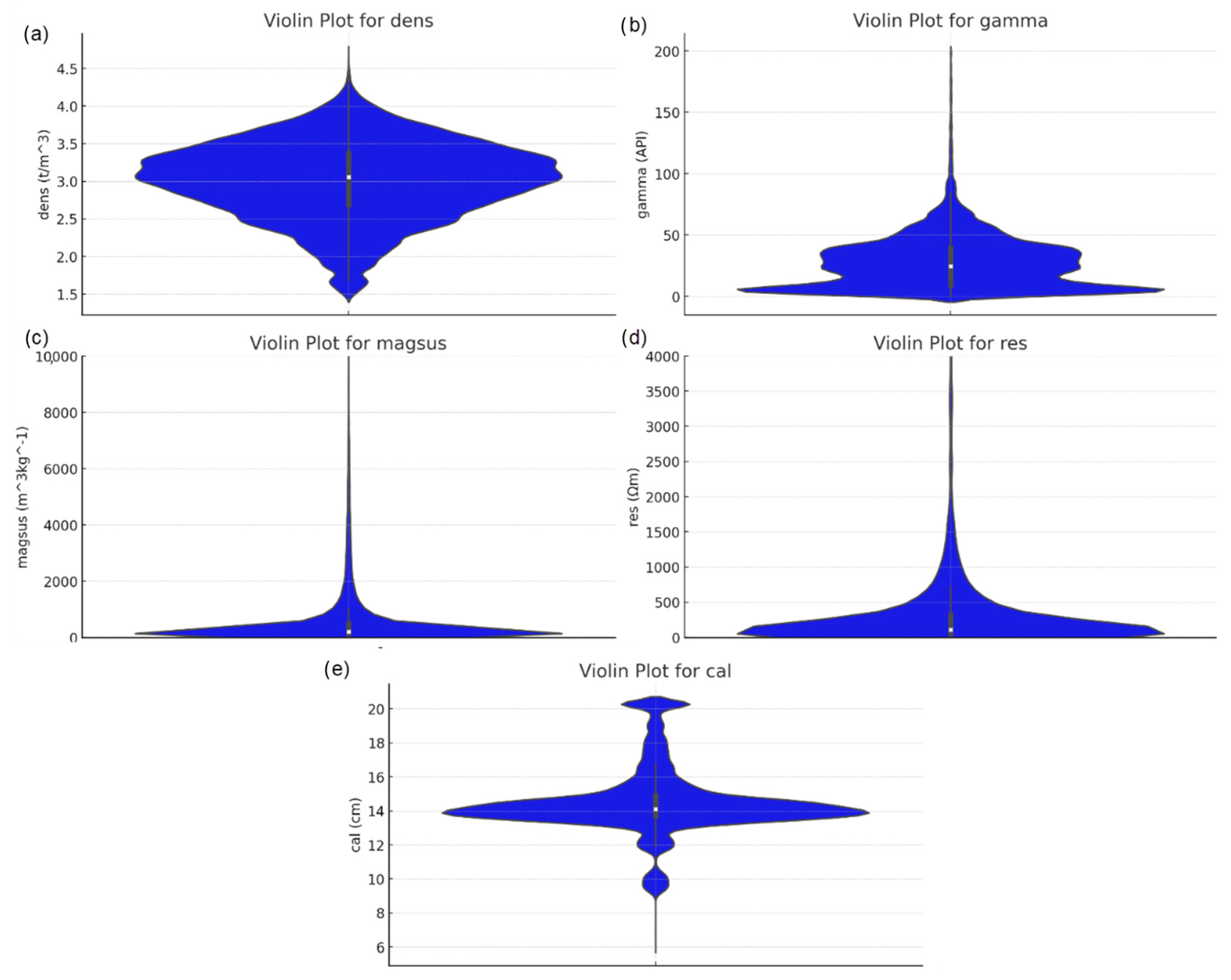
2.2. Geological Qualities from Geophysical Measurements
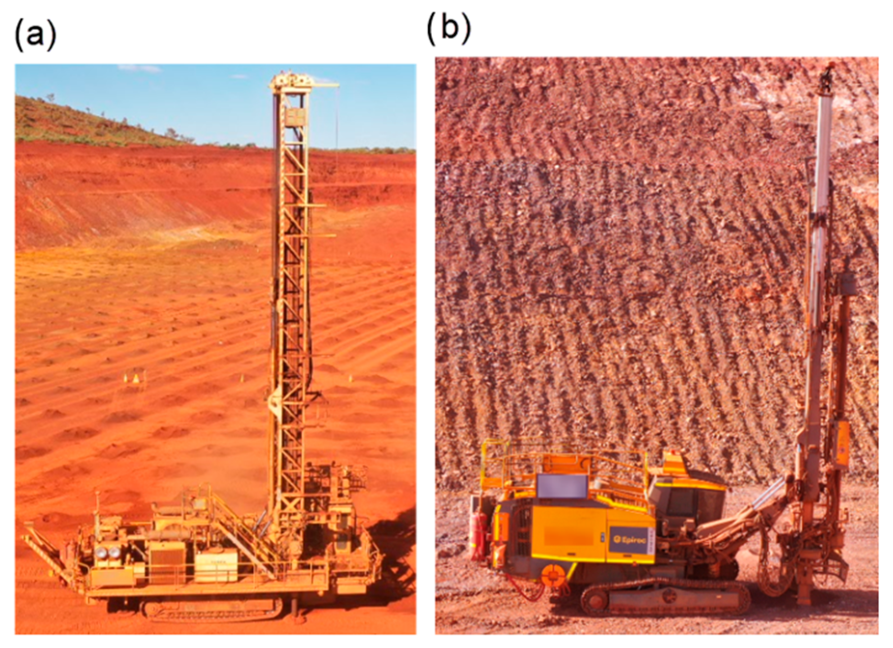
This study considers various geophysical measurements, namely radioactive (gamma and density), electrical (resistivity and magnetic susceptibility), and physical (hole diameter), which are measured from their respective downhole sondes. The numbers of observations used after data processing are listed in Table 1.
Gamma and density wireline logging uses an active radioactive source to assess the bulk densities of subsurface materials as well as their reactions to the gamma radiation emanating from a regulated source housed within the logging instrument [28]. These responses are used for several purposes. For example, density (dens) is predominantly used as a proxy for ore grade. It can also be employed to estimate the tonnage of overburden stripping or as a measure of porosity. In contrast, the prevalent association of gamma radiation with clay minerals has led to using gamma as an indicator of shale or clay.
Resistivity and magnetic susceptibility are types of electrical logging that measure the electrical attributes of a rock formation. Resistivity (res) defines its capacity to resist the flow of electric current. Alterations in the rock’s electrical properties can be attributed to factors, such as the content of clay minerals, water content and porosity, temperature variations, and conductivity of water [29]. Consequently, resistivity logs assist in interpreting conductive material properties and are predominantly employed to estimate salinity and demarcate lithology for hydrogeological studies. Magnetic susceptibility (magsus) quantifies the magnetization level of the stratigraphy in a drill hole when exposed to a magnetic field using electromagnetic induction [30]. magsus data are useful for characterizing the degree of magnetization of subsurface material encountered in a drill hole exposure to differentiate and infer the mineralogy or lithology of a formation.
The caliper (cal) log, also referred to as the hole diameter log, is a physical measurement tool in which one or more tensioned mechanical arms measure the dimensions of the drill cavity [28]. Certain physical characteristics of the drill hole, for example, hole diameter, hole wall roughness, and drilling mud thickness, influence other geophysical measurements. By interrogating the drill hole wall, cal can be used in conjunction with other geophysical measures to gain an improved understanding of subsurface geology.

2.3. MWD Systems

This research employed the MWD method for data collection, using a total of 22 rotary blast hole drill rigs that were outfitted with Tungsten Carbide Insert bits. The drilling fleet comprised ten Atlas Copco (Epiroc) Pit Viper 271 rigs, two Terex SKS 12 rigs, a single Bucyrus SKS 13 rig, and two Sandvik 460 rigs. These were deployed to drill production blast holes with a diameter of 0.229 m (Figure 1a). In addition, one Cubex QXR 920 rig, one Sandvik 560 rig, and five Atlas Copco (Epiroc) D65 drill rigs were deployed for drilling 0.165 m wall control blast holes (Figure 1b). The bench heights in the studied iron ore pits ranged from 8 to 12 m, with sub-drilling extending roughly 2 m below the bench floor. The spacing and burden between production blast holes averaged at 8 m and 7 m, respectively.
The MWD system on the drill rigs tracked metrics including the rate of penetration (rop; m/s), rotary pressure or torque (tor; Nm), force on bit (fob; kgf)—also called weight on bit, thrust, or pulldown pressure—bit air pressure or flushing air medium (bap; kgf/cm2), and rotary speed (rpm). However, due to irregularities in the onboard sensor, the rpm data were only available for approximately a quarter of the sample points, leading to the exclusion of rpm from the drilling variables. The collection of MWD metrics was facilitated by a mix of manually operated rigs and semi-autonomous machines, with the latter being remotely overseen from an off-site operations center. The drilling system logged the MWD time-series data at about 0.1 m intervals along the blast hole depth.
MWD data were collected from two distinct pits, BR and MM, each characterized by unique geological conditions. The BR provided a dataset encompassing 75,470 blast holes totaling 844,855 m, while the MM pit contributed a dataset comprising 18,887 holes totaling 208,705 m. A combined dataset (COM) was generated using BR and MM data. Combining datasets from different pits improves the robustness of the analysis and ensures that predictive models are applicable across different geological settings. This study concentrated on MWD data ranging from 2 m below the hole collars to the bottom of the blast holes, as the initial two meters of the borehole may not accurately represent the in situ geochemical properties of the rock due to possible toe charge effects during the previous bench’s blasting.

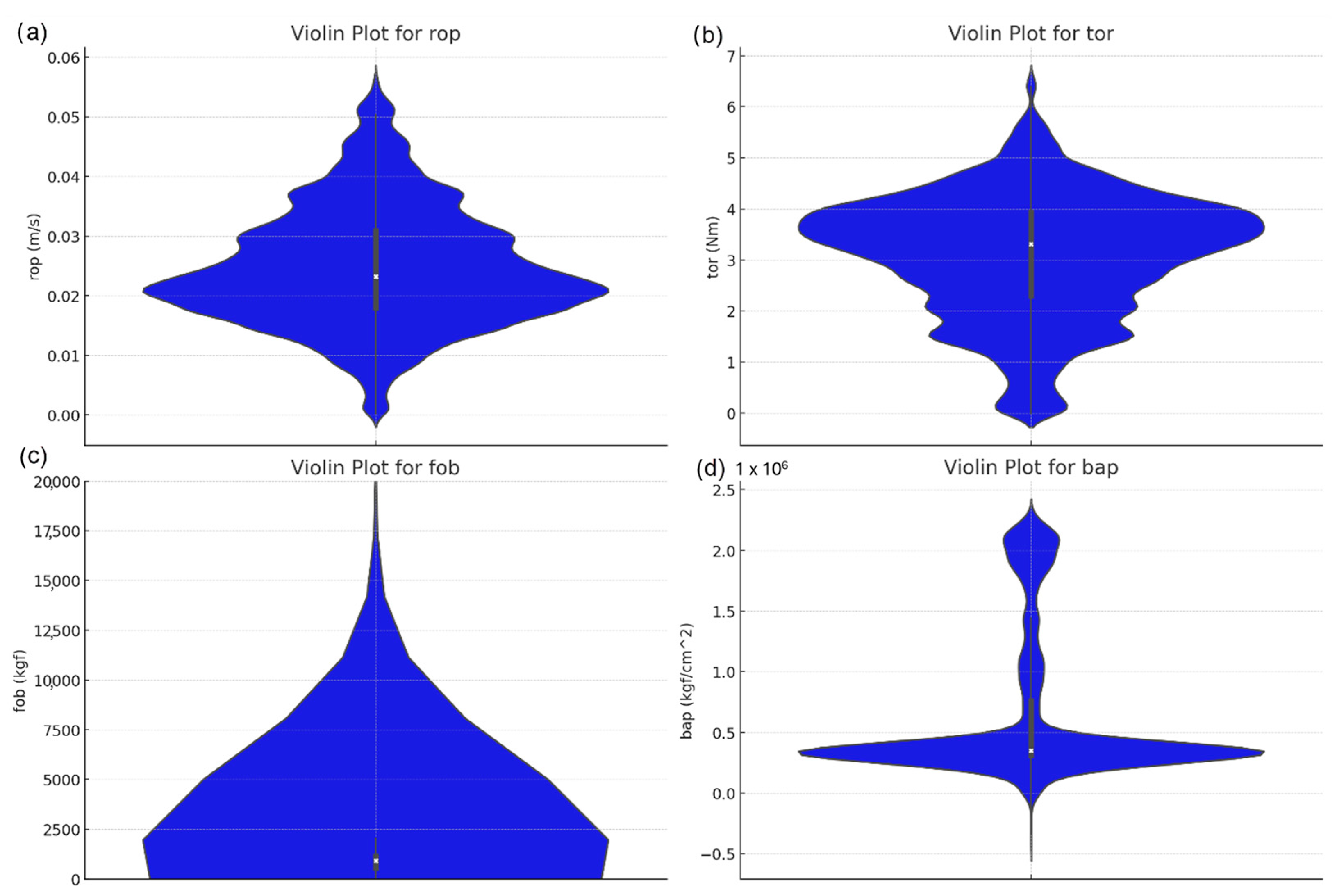
MWD Data Pre-Processing

The efficacy of MWD data is affected by a variety of factors, such as subsurface composition, drill rig management system, and external circumstances, which can result in abnormal response values [32]. Consequently, these discrepancies can potentially lead to inaccurate MWD response values and erroneous interpretations of the data [33]. Accordingly, the noise-to-signal ratio in the analyzed mining MWD dataset is substantial as the data had not been subjected to a thorough QA/QC process.
As a result, the MWD data in this study required feature engineering. Because collaring effects at the start of the shaft and potential blast damage from previous holes could skew the in situ rock representation, the initial MWD dataset omitted the first 2 m of each drilling hole. Then, any data points with negative rop, tor, fob, or bap values were removed. Using linear interpolation, interquartile range methods, and a 1.5-factor threshold, the voids in the MWD data were considered outliers and subsequently filled. The blasthole data were refined with a Gaussian filter smoothing factor of 0.3 to reduce the local impacts of noise.
The MWD features obtained after performing feature engineering on the first four MWD responses are shown in Table 2. These variables contain the original MWD features, derived ratios of the original features (e.g., rop divided by tor, indicated as roptor), and a moving standard deviation across 0.5 m for the original features (e.g., ropS).
The drilling datasets for blast hole MWD and the exploration hole were transformed from drill hole interval formats to point data, including geospatial coordinates and associated dataset values for each data point. The point data for exploration holes were generated utilizing downhole wireline logged desurvey data, which recorded the azimuth and dip of each hole every 10 m until the final depth. On the other hand, the blast hole MWD data were not desurveyed due to the production nature of the holes, and the location of each point was determined by presuming a straight line from the hole’s collar to its end. To merge these two datasets, a K-Nearest Neighbor distance-based search technique was used to calculate the distance between each point in the MWD and exploration data. Each exploration drilling data point was associated with the nearest MWD data point to conduct supervised machine learning. Horizontal and vertical distance thresholds were utilized to further refine the outcomes.

2.4. Feature-Importance-Based Methods

PCA has frequently been used to determine the most important MWD features [14,17,19,22,34]. In contrast, this study employs feature importance algorithms to establish the relative importance of each MWD variable identified for geophysical measurements such as dens, gamma, magsus, res, and cal. Non-parametric approaches, such as MARS and PPR, were applied to the pre-processed and merged BR, MM, and COM datasets. Both techniques do not make any assumptions on the relationships between the input and output variables. However, they evaluate feature significance differently.
MARS, a non-parametric approach to regression, disentangles complex variable interactions through a succession of piecewise linear regressions [35]. It identifies crucial features by fitting the model iteratively with each feature, both included and omitted, and measuring the performance variation. MARS has been demonstrated as a valid feature importance methodology in other fields, including molecular biology, environmental science, and civil engineering [36,37,38]. The MARS algorithm selects the MWD input that leads to the greatest improvement in the model as the most important as follows:
f ^ x = j = 1 J a j B j x
where f ^ x is a spline approximation of the function of interest f(x) given by respective constant coefficients, aj, and a linear combination of basis functions, Bj(x) for (j = 1, 2, …, J), which consist of a constant and a hinge function [36]. The earth package in R (v5.3.4), which uses the MARS technique, was used with default hyperparameters to generate models that match the data distribution and to assess the feature relevance of correlations between MWD variables [39].
On the other hand, PPR, a nonlinear regression technique, reveals the most informative data projections into a lower-dimensional subspace [40]. In contrast to MARS, it identifies the most influential characteristics by analyzing the impact of each variable on these projections and determining which variables contribute the most to informative estimates. PPR has been used extensively in other fields for feature importance, including geometallurgy, biochemistry, and economics [41,42,43]. The PPR formula is as follows:
f ^ x = m = 1 M S α m i = 1 n α i m x i
where α i m x i denotes the inner product iteratively created in three steps: (1) initializing the residual to the response variable and the term counter M to zero; (2) using numerical optimization to determine the S values that maximize the figure of merit; and (3) eliminating the last term if the merit score falls below a particular threshold. The R package stats (v3.6.2) [44], which incorporates PPR, was used with default hyperparameters to determine the goodness of fit for each variable.
MARS and PPR were utilized to quantify the feature importance of drilling metrics with the goal of understanding the complex, multi-variate relationships between MWD features and in situ geochemical signatures. These feature-importance-based methods were applied to MWD data for both short and big n-terms (basic functions of 101 and 201 for MARS, and terms of 5 and up to 50 for PPR, respectively). Furthermore, the purpose was to determine whether complex models with larger n-terms would model links between geochemical assays and MWD data better than simpler models with smaller n-terms.

2.5. Regression-Based ML Methods

Neural Networks (NNs) are the only regression-based ML algorithms that have been used to address subsurface geophysical intensity with moderate success [19]. However, this study employed a variety of regression-based ML techniques, including Support Vector Machines (SVMs), Random Forests (RFs), Gaussian Process Regression (GPR), Linear Regression (LR), and Decision Trees (DTs), to investigate the effectiveness of these models to correlate geophysical properties with MWD data, as shown in Table 3.
Su et al. defined LR as a simple linear model that attempts to fit a line to a given dataset [45]. LR works well when the input and output variables are linearly related. However, LR algorithms may miss complex multivariate relationships. In contrast, DTs use recursive partitioning and key attributes to divide the data into smaller subgroups [46]. These trees can efficiently capture nonlinear interactions, but improper pruning may lead to overfitting. SVMs seek to determine the optimal hyperplane for classifying data [47]. They can effectively manage nonlinear relationships and high-dimensional data using kernel methods. Breiman defines RFs as a combination of several DTs to improve efficiency, prevent overfitting, and manage nonlinear relationships [48]. GPR examines the output variable as a Gaussian distribution to identify the function that most closely approximates the data [49]. The GPR method considers nonlinear interactions and provides a probabilistic prediction of the outcome. Bishop describes NNs as flexible nonlinear models because they are modeled after the human brain, consisting of interconnected layers of neurons [50]. NNs reflect complicated relationships and work well with high-dimensional data but are susceptible to overfitting if not adequately regulated.
This study evaluated the predictive ability of regression-based ML algorithms and performed the calculations on a Pawsey Supercomputer Nimbus cloud Ubuntu instance with 8 vCPUs and 32 GB of memory. The Regression Learner Toolbox in MATLAB (R2024A) was used with default hyperparameters and no optimization for each respective regression-based ML method to generate models and assess prediction performance [51]. The coefficient of determination (R2) and root mean square error (RMSE) metrics were used to compare the performance of various models, defined by the following criteria:
R 2 = 1 R S S T S S = 1 i = 1 N y i f x i 2 i = 1 N y i y ¯ 2
R M S E = 1 N i = 1 N y i f ( x i ) 2
where RSS is the sum of squares of residuals, TSS is the total sum of squares, N is the sample size, y i is the measured value, f ( x i ) is the predicted value, and y ¯ is the mean.

3. Results

A preliminary investigation of the MWD features (rop, tor, fob, and bap) collected from sensors on the drills was conducted to comprehend the data’s range and frequency. Significant variations in rop and fob can be attributed many factors, including inconsistencies in mining equipment, operator competence, bit degradation, and rock mass properties [52]. Therefore, a single variable analysis of these features may not adequately capture the nonlinear correlations between MWD and geophysical measurements.
Figure 2a–d depict the first four MWD datapoints from the COM, respectively. The COM rop displayed a balanced distribution, averaging 0.0248 m/s with a standard deviation of 0.010 m/s. Similarly, as shown in Figure 2b, the COM tor responses also have a typical distribution, with a mean of 3.41 Nm and a standard deviation of 1.06 Nm. On the other hand, Figure 2c depicts the skewed distribution of the COM fob with a mean of 97,945 kgf and a standard deviation of 78,524 kgf. Figure 2d displays a normal distribution for the COM bap, with values ranging from 230,300 kgf/cm2 to 439,400 kgf/cm2, a mean value of 335,550 kgf/cm2, and a standard deviation of 49,384 kgf/cm2.
Upon examination of the COM geophysical data presented through violin plots in Figure 3, distinct patterns were observed. The COM dens measurements exhibit a uniform distribution, suggesting consistent rock densities across the studied region. In contrast, the COM res data are notably skewed towards lower values, indicating predominant low resistivity, with occasional higher resistivity regions. In addition, the COM gamma and COM magsus measurements present more variable distributions, signifying a diverse range of rock properties. Lastly, the COM cal data demonstrate symmetry, indicating consistent borehole sizes. While certain measurements like dens and cal indicate uniformity, gamma and magsus highlight variability in subsurface geophysical conditions.

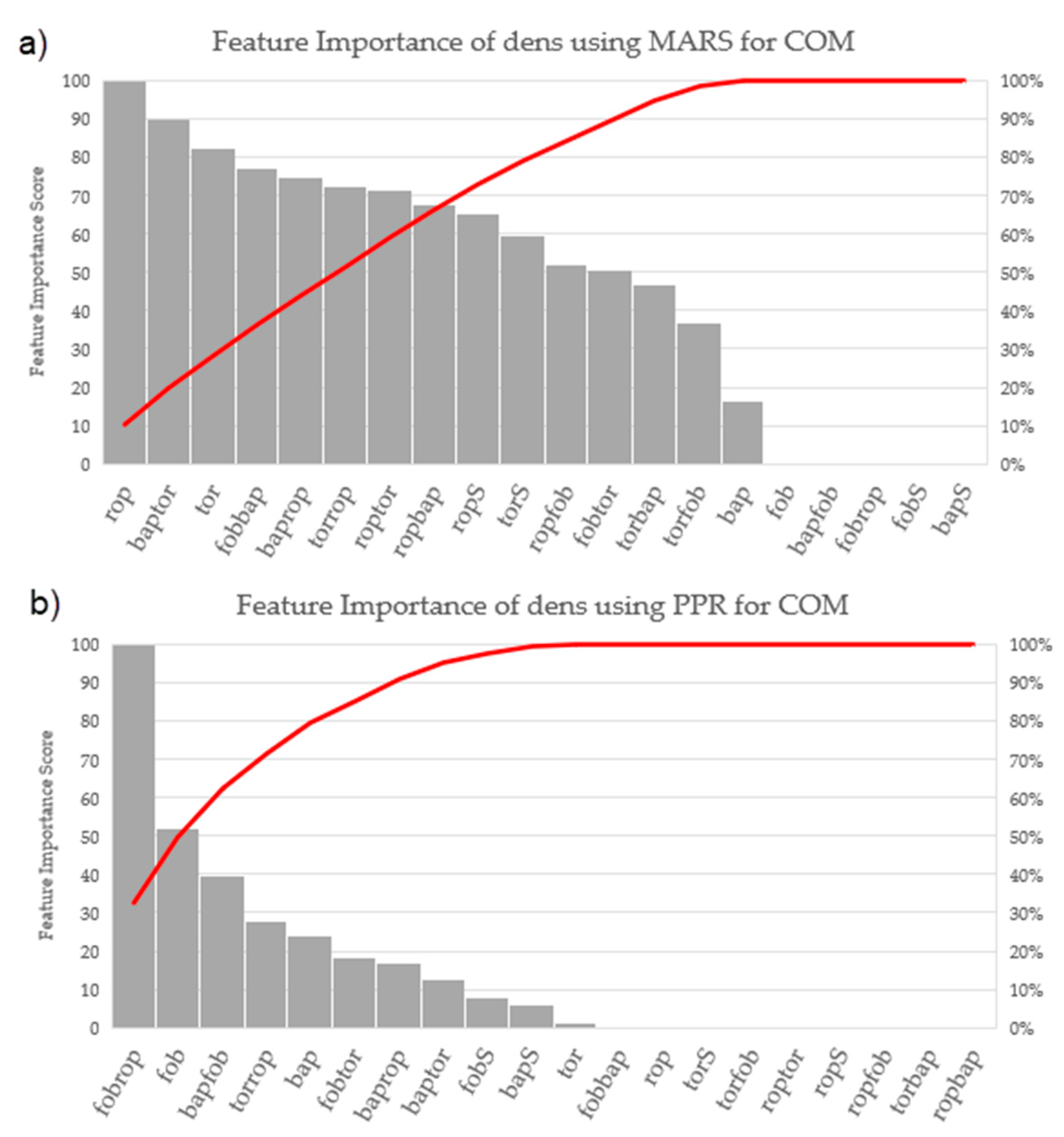
3.1. Feature-Importance-Based Results

The importance of the investigated MWD response features in inferring geophysical measures was investigated. Small and large n-terms MARS and PPR models were developed to determine whether more complex ML methods would be advantageous during subsequent predictive modeling.
The percentages presented in Table 4 and Table 5 were calculated by adding the relative weights of each attribute and dividing by the total for MARS and PPR, respectively. These percentages can be categorized into three different groups: (a) 0% relative feature importance, where MWD features were deemed irrelevant by MARS and PPR in predicting orebody quality measures; (b) greater than 0% but less than 5% relative feature importance (minor importance), indicating a slight influence on the prediction of orebody quality measures; and (c) exceeding 5% relative feature importance.
The findings suggest that the relative importance of features remains stable across models with both small and large term counts. Despite the apparent consistency in both n-term models, MARS and PPR analyses assigned varying degrees of importance to different features. For instance, when using the COM dataset, the MARS method identified 15 out of 20 of the MWD measures as crucial in inferring dens (Figure 4a), with the exceptions being fob, bapfob, fobrop, fobS and bapS. Most features were identified as important due to the MARS method, which involves searching for relationships between variables. Conversely, the PPR approach determined that only half of the MWD features were important, with only five variables being greater than or around ten percent: fobrop, fob, bapfob, torrop, and bap. (Figure 4b). PPR implies that the remaining MWD features exert minimal to no influence on the prediction of orebody quality, possibly due to the lack of consideration for nonlinear interaction among features in the PPR model. Thus, to encompass all potential significant MWD features, MARS and PPR methodologies were employed.
Figure 5 provides a comparative analysis of the significance of the MWD features for gamma, dens, magsus, res, and cal COM dataset, as determined by the MARS and PPR methodologies. These results correspond to the top ten most important MWD features discovered in the dens analysis (Figure 4). The MWD characteristic fobrop routinely emerges as highly important in this study’s datasets, along with bapfob, baprop, fob, bap, and fobtor. It is important to note, however, that this does not diminish the importance of other MWD features; rather, it highlights those that are frequently identified as important.
As shown in Table 4 and Table 5, the importance of features for evaluating dens varies across different datasets when the MARS and PPR methodologies are applied. The six MWD variables deemed most important for predicting den from the analyzed BIF deposits are fobrop, fobtor, bapfob, torrop, baprop, and baptor, in accordance with the peak importance findings (Figure 5). This result generally corresponds to the importance of MWD features identified for gamma, magsus, res, and cal (Figure 4). The ratios fobrop, fobtor, bapfob, torrop, baprop, and baptor carried more importance than the primary rop and tor variables, the rop-influenced ratios roptor, ropbap, and ropfob, as well as the variability-related metrics ropS, torS, and bapS. On the other hand, fob was identified as highly important from PPR but was very low or missing in the MARS rankings.

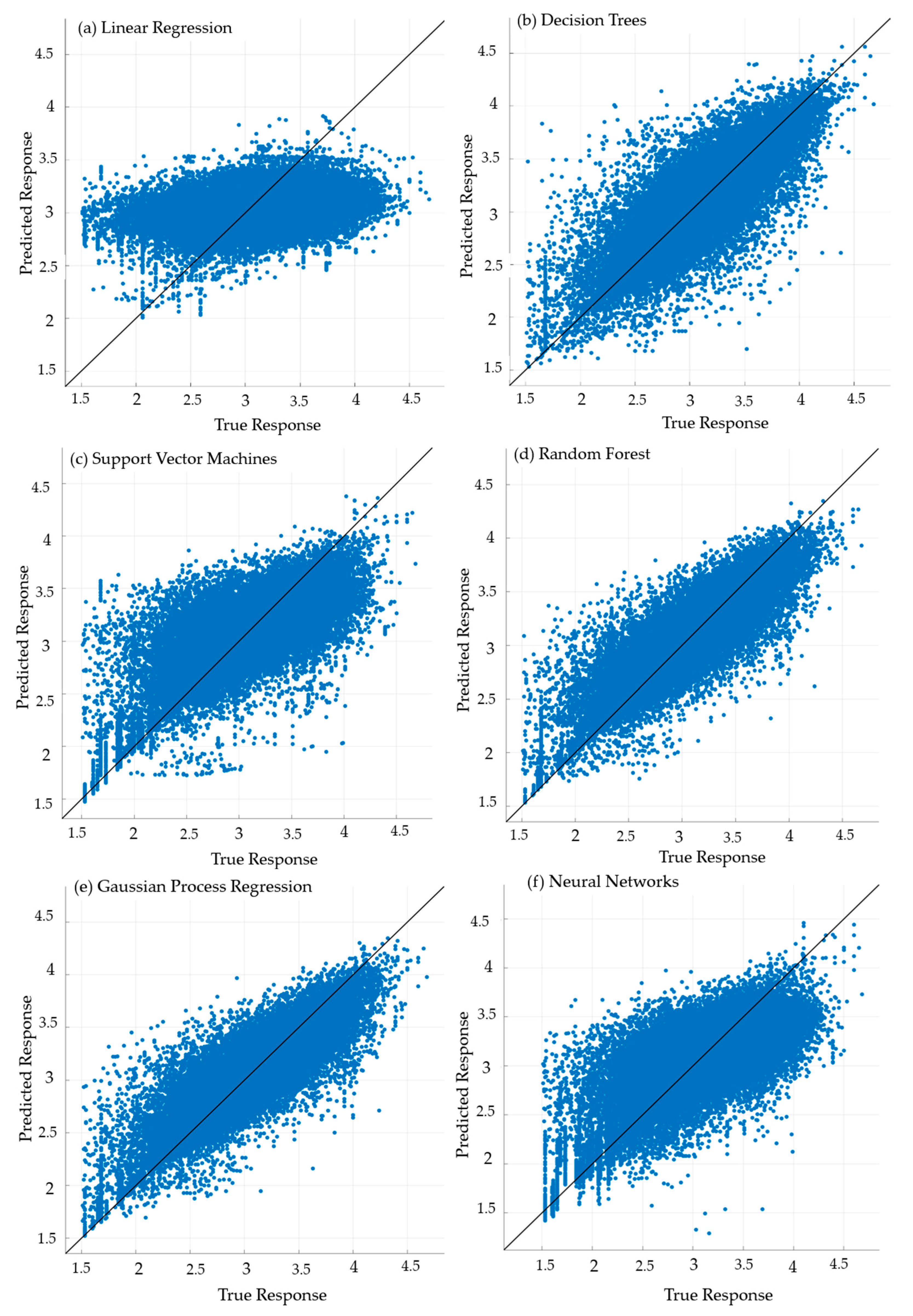
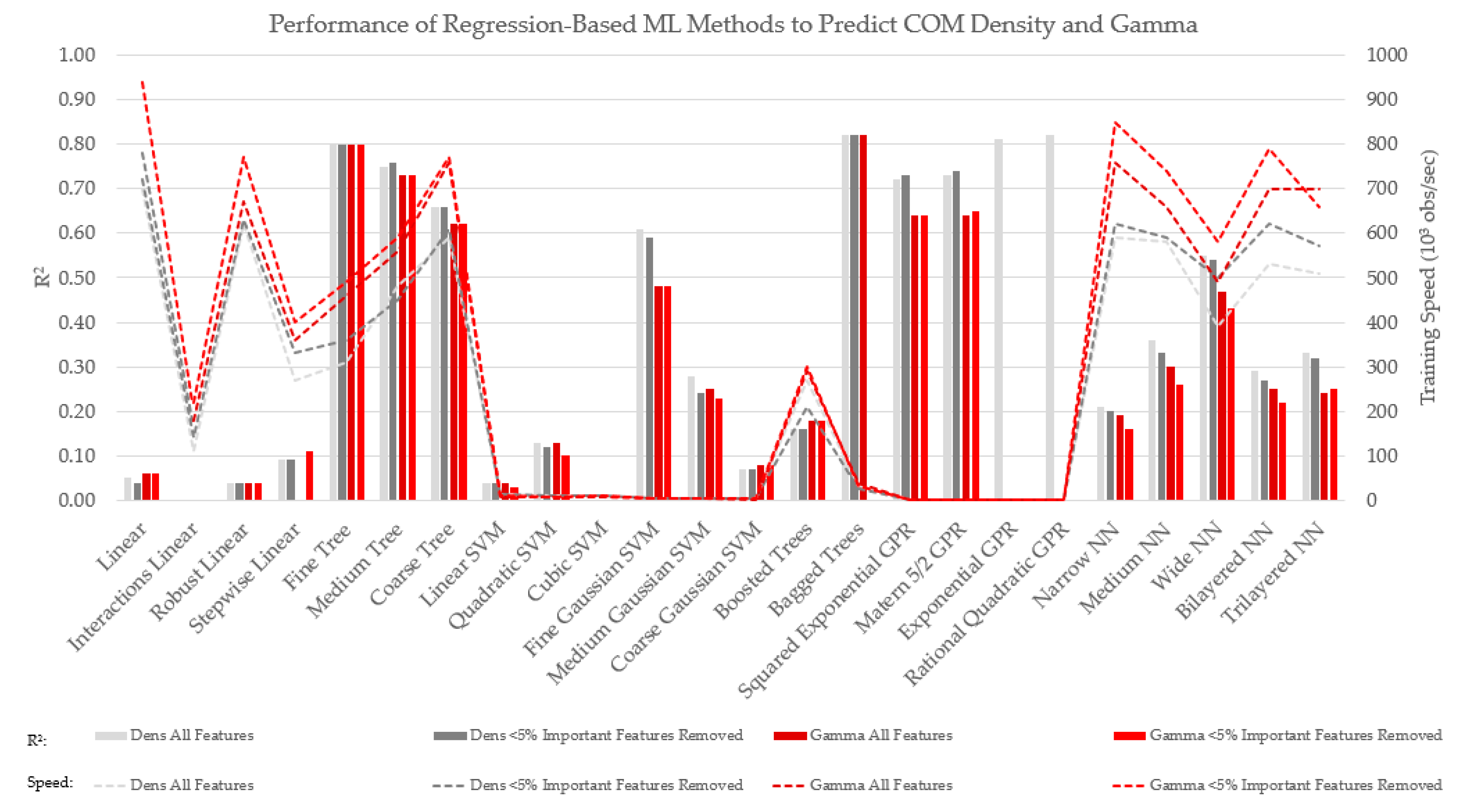
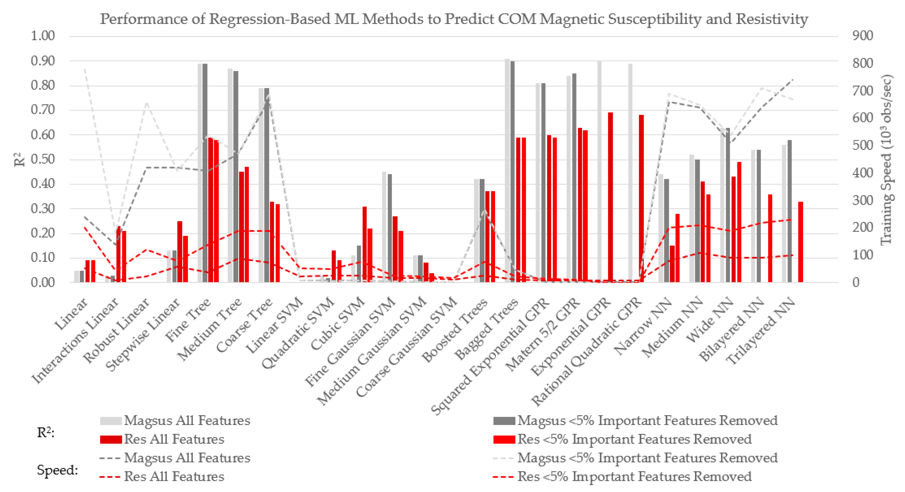
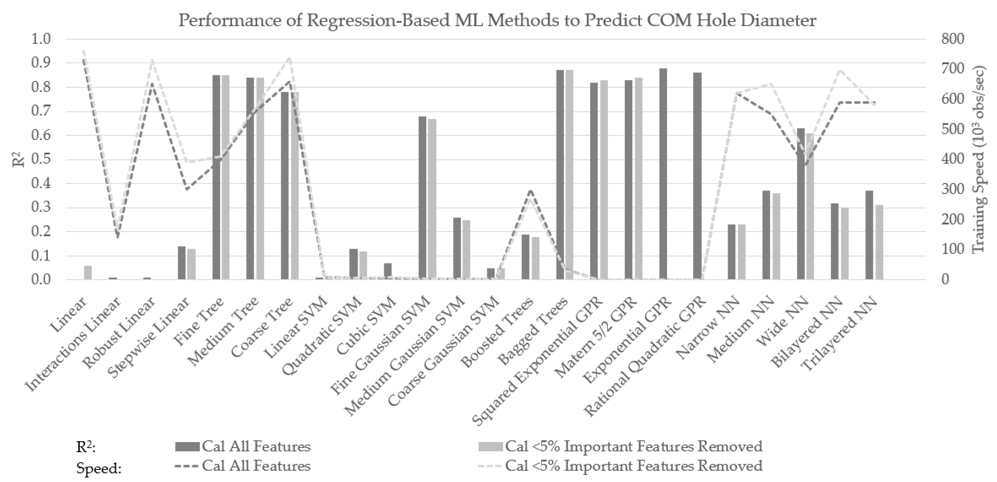
3.2. Regression-Based ML Analytical Prediction Results

The following sections evaluate the prediction strength of several kinds of regression-based ML regression models for predicting geophysical measurements of an orebody. The investigated geophysical measurements included dens, gamma, magsus, res, and cal, and they were predicted based on the MWD input features described in Table 2. This analysis required validating the proposed ML analytical procedure with a variety of geophysical signatures to establish theoretical precision.
A 10-fold cross-validation technique revealed the training dataset’s prediction strength. The datasets were split into 80% for training and 20% for testing. The testing results are reported as RMSE value, with the R2 value being the average of the 10 folds during cross-validation. In addition, a threshold of twenty-four hours of computation time was established due to practical limitations regarding calculation speed for real-time analysis. Consequently, several GP-based analyses were prematurely terminated and categorized as nonapplicable (N/A). Moreover, scatter plots are useful for visualizing individual predictions but may not effectively convey comparative model performance across multiple geophysical parameters. Tables provide a comprehensive view of RMSE and R2 across different models, allowing for a direct evaluation of their relative strengths and weaknesses.
A preliminary investigation was conducted using the Coarse DT method to determine whether additional MWD features beyond rop, tor, fob, and bap would strengthen the prediction performance of regression-based ML models. The results are listed in Table 6. Based on these results showing that 14 out of 15 models performed better with the additional features, the decision was made to incorporate the ratio and moving standard deviation (Table 2) MWD features in all of the investigated predictive ML models. The res models did not improve as much as the others, possibly due to smaller numbers of observations due to this geophysical sonde not being used in every drillhole.

3.2.1. Density and Gamma Prediction

The regression results for estimating dens and gamma values using ML models such as LR, DTs, SVMs, RFs, GP, and NNs are detailed in Table 7 and Table 8, respectively. The R2 values of models utilizing BR data to predict dens and gamma were marginally superior to those utilizing MM and COM datasets. This discrepancy may be attributable to the BR and MM datasets containing different quantities of data.
Among all COM models, those employing LR and SVMs consistently produced the least accurate predictions for dens and gamma with R2 values below 0.50 (Table 7 and Table 8). In contrast, models constructed with DTs, RFs, and GP yielded the highest R2 values for dens and gamma predictions, with both achieving 0.80. These high-performing DTs, RFs, and GP models yielded an average RMSE of approximately 0.21 t/m3 for dens and 9.42 API for gamma. GP displayed the most accurate predictions, with R2 values of 0.87 and 0.92 and RMSEs of less than 0.19 t/m3 and 6.32 API for MM dens and gamma, respectively.
Within each ML algorithm class, significant differences were observed between the subclasses of ML outlined in Table 3. As an example, the Bagged (Bootstrapped Aggregate) Tree method outperformed the Boosted Tree RFs in predicting densities and gamma, with an R2 value of approximately 0.82 for both geophysical measurements. Similarly, Wide NNs consistently outperformed other NN types, with peak R2 values of 0.54 and 0.43 for dens and gamma, respectively, and the lowest RMSE values of 0.35 t/m3 for dens and 16.68 API for gamma. Lastly, a Fine Tree DT correlation value of 0.80 for both dens and gamma was obtained, which is superior to those of the Medium and Fine parameters.
Figure 6a–f depict the ML analytical prediction results compared to actual wireline measured dens values for the best-performing LR, DTs, SVMs, RFs, GP, and NNs models. The Bagged RF models had the strongest correlation with an R2 value of 0.82. The DT models generated a slightly weaker R2 value of 0.80. However, the training speed of the DT models was over 10 times that of the Bagged RF models, at around 400 with 35 observations per second, respectively. Furthermore, although density is often considered a relatively stable parameter, its prediction using MWD data remains complex due to inherent sensor noise, operational variability, and small-scale geological heterogeneity. The errors observed in Figure 6 reflect these real-world challenges, reinforcing the need for further data integration approaches.
In addition, a series of three-level experiments with variable input parameters were conducted to correspond to the three primary levels of relative feature significance determined by MARS and PPR in Section 3.1, namely 0%, less than 5%, and over 5%. The objective of this method was to determine the effect of omitting MWD features deemed to be of minimal importance. The experimental design included (1) all 20 MWD features, including those with 0% relative importance, (2) the exclusion of MWD features identified as having 0% relative importance, and (3) the removal of MWD features classified as having less than 5% importance, which was designated as minor importance.
Interestingly, the elimination of minor importance features had no effect on prediction performance when compared to the use of all features (Figure 7). With the gamma COM dataset, most instances exhibited less than a 0.05 decrease in R2, whereas the Fine Tree and Medium Tree DT techniques demonstrated 0.19 and 0.06 enhancements in R2, respectively. Nonetheless, there was a consistent increase in training speed for dens and gamma DTs, as well as dens NNs, when marginally significant features were used over all features (Figure 7). In contrast, when utilizing all features, gamma NNs models demonstrated faster training rates and higher R2 values. This anomaly may be due to the inherent dynamics of the NN method, which has difficulty establishing relationships between these datasets using marginally significant features, resulting in lower R2 values.

3.2.2. Magsus and Res Prediction

The prediction results of magsus and res geophysical measurements using various ML models, including LR, DTs, SVMs, RFs, GP, and NNs, are presented in Table 9 and Table 10. Interestingly, the DT models showed consistent performance across the BR, MM, and COM datasets, with R2 variances of less than 0.02 between them. In contrast, the NN models demonstrated a notable performance improvement on the MM dataset. This divergence aligns with the observations made for dens and gamma (see Section 3.2.1) and could be attributed to the disparity in data volume between the BR and MM datasets, a point that requires more investigation.
The DT approaches produced R2 values ranging from 0.79 to 0.89 when applied to COM magsus data. However, the res COM DT models were remarkably lower than the magsus data, ranging from 0.32 to 0.58. This discrepancy could be due to the res dataset having around 10 times less data due to inconsistent wireline logging practices, as res was not measured on the same number of holes as magsus. Moreover, the relatively weak prediction performance of res can be attributed to the lack of intrinsic correlation between drilling parameters and resistivity in formations devoid of conductive minerals. Since res primarily depends on pore fluid content rather than mechanical drilling forces, ML models face inherent challenges in accurately modeling this relationship.
Certain ML subclasses outperformed others within the same ML class, a pattern consistent with those discovered for dens and gamma. For example, Fine DTs consistently outperformed Medium and Coarse DTs in both the COM magsus and res datasets. Moreover, in the predictions for magsus and res, Bagged RFs performed better than Boosted Tree RFs. Likewise, Wide NNs consistently outperformed other NN subclasses, with the R2 values for magsus and res reaching maximums of 0.63 and 0.49, respectively. Fine Gaussian SVMs achieved R2 values greater than 0.44 for magsus and Cubic SVMs of 0.22 for res, demonstrating a wide range of outcomes. In contrast, the R2 values of Linear and Coarse Gaussian SVMs were all 0.00.
With R2 values exceeding 0.60 for electrical geophysical predictions, GPs consistently generated reliable results across all GP subclasses. Nonetheless, as shown in Figure 8, GP models required a prolonged computation time than methods such as DTs, RFs, and NNs. However, no significant decrease in prediction performance was observed when models excluded features with less than 5% importance in comparison to models that included all features. Certain models, including most created with Stepwise LR, Exponential GPR, and Rational Quadratic GPR, had to be stopped after 24 h; therefore, their results are not included here.

3.2.3. Caliper Predictions

Table 11 displays the results of cal prediction using the LR, DT, SVM, RF, GP, and NN models. The BR, MM, and COM models all had relatively consistent R2 and RMSE values. These results contrast with the differences between the BR and MM observed in the dens, gamma, magsus, and res results, indicating the need for an additional investigation to understand the differences between the BR and MM results.
Examining the predictive performance of these models reveals that all variants of LR models, including Linear, Interactions, Robust, and Stepwise, consistently underperformed with R2 values lower than 0.45. In contrast, models built with SVMs, RFs, GP, and NNs provided more accurate predictions, with maximum R2 values of 0.86, 0.89, 0.92, and 0.87, respectively, and an average RMSE of approximately 0.63 cm.
Among these models, Bagged RFs and Wide NNs delivered the best predictive results within their respective ML classes, with RMSEs of 0.62 cm and 0.68 cm, respectively. On the COM dataset, DTs produced R2 values of 0.76, 0.80, and 0.94 for the Coarse, Medium, and Fine parameters, respectively. SVMs displayed the most variable results based on the chosen method, with Fine Gaussian achieving an R2 value of up to 0.86 and Linear, Cubic, and Coarse Gaussian yielding R2 values below 0.50 and a 1.34 cm RMSE.
Experiments that excluded features with less than 5% (minor) importance had no appreciable impact on the cal prediction accuracy. Compared to the trials that included all MWD features, as shown in Figure 9, this feature exclusion sped up the model training times. DTs and NNs emerged as the quickest training methods with around 600,000 observations per second, whereas GP computations were around 300× more time-consuming with around 2000 observations per second. The models utilizing Exponential GPR (for BR < 5% and MM < 5%) and Rational Quadratic GPR (for BR < 5%, MM < 5%, COM all, and COM < 5%) were discontinued after 24 h, and their results are therefore not presented.

4. Discussion

This study demonstrates the effectiveness of feature-importance-based methods and regression-based ML techniques in estimating subterranean geophysical signatures from MWD data, thereby increasing orebody knowledge. Table 4 and Table 5 reveal that the success of predictive modeling of the five investigated geophysical properties depends primarily on two factors: the characteristics of the on-site host rock, as represented by MWD data, and its distribution across various mining locations, as well as the quantity of data. While the absolute predictive accuracy of some models remains limited, this study provides crucial insights into which MWD variables contribute the most to predictive performance. These findings can guide future work in refining data preprocessing, feature selection, and hybrid modeling approaches that integrate geophysical constraints.
The impact of data volume (Table 1) is particularly significant, as greater amounts of MWD data improve the robustness and generalizability of regression-based ML models. Conversely, in scenarios with lower data availability or reduced data resolution, model performance may degrade, raising the question of whether alternative approaches might be more suitable. Future work should investigate the minimum viable amount of MWD data required for this approach to remain effective, particularly in settings where data sparsity is a constraint. Moreover, for parameters like resistivity, where intrinsic geological correlation with MWD features is weak, ML models struggled to achieve high predictive accuracy. This highlights the necessity of incorporating domain knowledge when interpreting ML outputs.
Though the scope of this study was confined to five geophysical properties, it has the potential to be extended to other measurements such as acoustic, neutron porosity, dip-meter, spontaneous potential, or nuclear magnetic resonance. This study departs from prior research by showing the importance of MWD ratio features, such as fobrop, fobtor, bapfob, torrop, baprop, and baptor, in addition to fob. Earlier research emphasized rop and tor, utilizing PCA to determine the most important MWD measurements for rock type identification [9,12,14,17,19,34]. In contrast with the PCA-based feature selection in MWD data, feature-importance-based ML methodologies, such as MARS and PPR, revealed previously unobserved complex relationships between MWD features and rock mass characteristics such as those derived from bap.
The differences in feature importance evaluations between MARS and PPR result from the underlying mechanics of these algorithms. The MARS technique evaluates the correlation between MWD features and geophysical signatures, therefore expanding the range of relevant MWD features (Table 4). On the other hand, PPR evaluates the influence of each feature on data projections and determined that half of the drilling features were not important (Table 5).
Moreover, when compared to their smaller equivalents, larger n-term MARS and PPR models did not offer a more robust depiction of correlations between MWD data and geophysical measurements [53]. The consistent performance of DTs and Bagged RFs, with R2 prediction values exceeding 0.80 across most ML models, as shown in Table 7, Table 8, Table 9, Table 10 and Table 11, suggests that complex ML models may not always provide superior predictive capabilities. Furthermore, more complex models like SVMs struggle with non-scaled features and imbalanced datasets where one class of features dominates. In this case, the drill rig type and hole diameter may be two factors, as the larger rigs drilled more wider-diameter production holes than smaller rigs drilling narrower holes for wall control.
This study also examined regression-based ML model prediction performance when minor importance features were eliminated for approximating geophysical signatures. It was found that discarding MWD features of minor significance could increase the processing speed without significantly compromising prediction accuracy. The predictive performance of most models remained stable when less important features were omitted. Despite a slight decline in predictive performance, the accelerated training durations for larger datasets suggest that excluding less important features is advantageous.
In addition, the choice of the regression-based ML analytical model, whether GP, NNs, or RFs, had little effect on the ML prediction outcomes, indicating that the predictive accuracy was primarily dependent on the quality of the extracted features. This observation is consistent with the findings, which observed comparable prediction abilities among diverse ML models for rock types and geochemical assay results [8,18,31]. In particular, the prediction accuracy of geophysical measurement estimates for dens, gamma, magsus, res, and cal using DTs, SVMs, RFs, GPs, and NNs models in the BR dataset was much higher than in the MM or COM datasets. A great deal of these variances can be traced to differences in data volume between the two datasets. The differences in geological composition between the Brockman and Marra Mamba Formations may also account for the residual differences in predictive power between BR and MM studies.

5. Conclusions

This study introduced a method for evaluating subsurface geophysical characteristics by applying feature-importance-based methods and regression-based ML algorithms to MWD data. The ability of feature-importance-based methods to unveil the “black box” nature of ML methods enable greater interpretation and acceptance of these models. A framework was developed to assess the importance of MWD data features in estimating the geophysical properties of an orebody, including density, gamma, magnetic susceptibility, resistivity, and hole diameter. Through MARS and PPR feature importance analyses, MWD features were grouped based on their importance as negligible (0%), minor (<5%), or significant (>5%). Notably, several previously unrecognized MWD attributes, such as fob, and ratios derived from MWD features—fobrop, fobtor, bapfob, torrop, baprop, and baptor—were found to have significant importance in determining geophysical attributes. Future work will also be extended to the use of other feature importance algorithms, such as Shapley value regression, which are increasingly used as tools in variable importance analysis in other fields [54,55].
Considering the varying importance of MWD features, we compared the prediction performance of various regression-based ML analytical methodologies, omitting specific features at distinct levels, considering the varying importance of the MWD features. The results indicate that omitting MWD attributes classified as having zero to minor importance does not significantly diminish prediction accuracy. Therefore, the elimination of features with low importance can reduce computation time without compromising the accuracy of the ML model’s estimates. In addition, empirical data revealed correlations as high as 0.91 between MWD attributes and orebody geophysical predictive values when RF was employed, validating the effectiveness of the proposed method.
Despite limitations in prediction accuracy, this study establishes a foundation for MWD-based geophysical modeling, demonstrating the feasibility of ML applications while identifying areas requiring further refinement. Future advancements in feature engineering and hybrid modeling approaches may enhance practical applicability. While this study highlights that ML provides powerful predictive capabilities, its utility is maximized when combined with geological expertise to validate and interpret results appropriately.
These findings have significant implications for the mining industry. By utilizing these models, mining professionals can estimate precise and reliable short-term ore and waste tonnages. This predictive comprehension of orebody geophysical characteristics is crucial for mining operations as it guides extraction and processing decisions. The high-resolution geological data derived from these models enable the recovery of high-grade ore containing economically valuable minerals. Through the high-resolution orebody representation afforded by the methodologies outlined in this study, mining geologists could better distinguish between high-grade, low-grade, and waste components. As a result, mining engineers can develop optimal excavation strategies that minimize the amount of waste material incorporated into processing facilities.

Author Contributions

Conceptualization, D.G.; methodology, D.G.; software, D.G.; validation, D.G.; formal analysis, D.G.; investigation, D.G.; resources, D.G.; data curation, D.G.; writing—original draft preparation, D.G.; writing—review and editing, D.G., C.A., Q.S. and L.O.; visualization, D.G.; supervision, C.A., Q.S. and L.O.; project administration, D.G. All authors have read and agreed to the published version of the manuscript.

Funding

This research received no external funding.

Data Availability Statement

The data used in this study is not publicly available due to confidentiality agreements with the organization that supplied it. Access to the data is restricted to comply with contractual obligations and proprietary considerations. As such, the dataset cannot be shared or disclosed.

Acknowledgments

One of the authors (D.G.) received support through the MRIWA Postgraduate Research Scholarship and the AusIMM Education Endowment Fund Postgraduate Scholarship during his doctoral studies at Curtin University. Furthermore, this research was enabled by the advanced computing resources provided by the Pawsey Supercomputing Research Centre in Perth, Australia.

Conflicts of Interest

The authors declare no conflicts of interest.

References

  1. Silversides, K.; Melkumyan, A.; Wyman, D.; Hatherly, P. Automated Recognition of Stratigraphic Marker Shales from Geophysical Logs in Iron Ore Deposits. Comput. Geosci. 2015, 77, 118–125. [Google Scholar] [CrossRef]
  2. Wedge, D.; Hartley, O.; McMickan, A.; Green, T.; Holden, E.J. Machine Learning Assisted Geological Interpretation of Drillhole Data: Examples from the Pilbara Region, Western Australia. Ore Geol. Rev. 2019, 114, 103118. [Google Scholar] [CrossRef]
  3. Barr, M.V. Instrumented Horizontal Drilling for Tunnelling Site Investigation. Ph.D. Thesis, University of London, Imperial College of Science and Technology, London, UK, 1984. [Google Scholar]
  4. Hatherly, P.; Leung, R.; Scheding, S.; Robinson, D. Drill Monitoring Results Reveal Geological Conditions in Blasthole Drilling. Int. J. Rock Mech. Min. Sci. 2015, 78, 144–154. [Google Scholar] [CrossRef]
  5. Khorzoughi, M.B. Use of Measurement While Drilling Techniques for Improved Rock Mass Characterization in Open-Pit Mines. Master’s Thesis, University of British Columbia, Vancouver, BC, Canada, 2011. [Google Scholar]
  6. Navarro, J.; Sanchidrian, J.A.; Segarra, P.; Castedo, R.; Paredes, C.; Lopez, L.M. On the Mutual Relations of Drill Monitoring Variables and the Drill Control System in Tunneling Operations. Tunn. Undergr. Space Technol. 2018, 72, 294–304. [Google Scholar] [CrossRef]
  7. van Eldert, J.; Schunnesson, H.; Johansson, D.; Saiang, D. Application of Measurement While Drilling Technology to Predict Rock Mass Quality and Rock Support for Tunnelling. Rock Mech. Rock Eng. 2020, 53, 1349–1358. [Google Scholar] [CrossRef]
  8. Kadkhodaie-Ilkhchi, A.; Monteiro, S.T.; Ramos, F.; Hatherly, P. Rock Recognition from MWD Data: A Comparative Study of Boosting, Neural Networks, and Fuzzy Logic. IEEE Geosci. Remote Sens. Lett. 2010, 7, 680–684. [Google Scholar] [CrossRef]
  9. Galende-Hernández, M.; Menéndez, M.; Fuente, M.J.; Sainz-Palmero, G.I. Monitor-While-Drilling-Based Estimation of Rock Mass Rating with Computational Intelligence: The Case of Tunnel Excavation Front. Autom. Constr. 2018, 93, 325–338. [Google Scholar] [CrossRef]
  10. Klyuchnikov, N.; Zaytsev, A.; Gruzdev, A.; Ovchinnikov, G.; Antipova, K.; Ismailova, L.; Muravleva, E.; Burnaev, E.; Semenikhin, A.; Cherepanov, A.; et al. Data-Driven Model for the Identification of the Rock Type at a Drilling Bit. J. Pet. Sci. Eng. 2019, 178, 506–516. [Google Scholar] [CrossRef]
  11. Peck, J.P. Performance Monitoring of Rotary Blasthole Drills. Ph.D. Thesis, McGill University, Montreal, QC, Canada, 1989. [Google Scholar]
  12. Scoble, M.J.; Peck, J.; Hendricks, C. Correlation between Rotary Drill Performance Parameters and Borehole Geophysical Logging. Min. Sci. Technol. 1989, 8, 301–312. [Google Scholar] [CrossRef]
  13. Segui, J.B.; Higgins, M. Blast Design Using Measurement While Drilling Parameters; Fragblast: Hunter Valley, NSW, Australia, 2001; pp. 28–31. [Google Scholar]
  14. Navarro, J.; Seidl, T.; Hartlieb, P.; Sanchidrián, J.A.; Segarra, P.; Couceiro, P.; Schimek, P.; Godoy, C. Blastability and Ore Grade Assessment from Drill Monitoring for Open Pit Applications. Rock Mech. Rock Eng. 2021, 54, 3209–3228. [Google Scholar] [CrossRef]
  15. Akyildiz, O.; Basarir, H.; Vezhapparambu, V.S.; Ellefmo, S. MWD Data-Based Marble Quality Class Prediction Models Using ML Algorithms. Math. Geosci. 2023, 55, 1059–1074. [Google Scholar] [CrossRef]
  16. Basarir, H.; Wesseloo, J.; Karrech, A.; Pasternak, E.; Dyskin, A. The Use of Soft Computing Methods for the Prediction of Rock Properties Based on Measurement While Drilling Data. In Proceedings of the Eighth International Conference on Deep and High Stress Mining, Perth, WA, Canada, 16–18 November 2017; pp. 537–551. [Google Scholar] [CrossRef]
  17. Beattie, N. Monitoring-While-Drilling for Open-Pit Mining in a Hard Rock Environment. Master’s Thesis, Queen’s University, Kingston, ON, Canada, 2009. [Google Scholar]
  18. Khushaba, R.N.; Melkumyan, A.; Hill, A.J. A Machine Learning Approach for Material Type Logging and Chemical Assaying from Autonomous Measure-While-Drilling (MWD) Data. Math. Geosci. 2021, 54, 285–315. [Google Scholar] [CrossRef]
  19. Martin, J. Application of Pattern Recognition Techniques to Monitoring-While-Drilling on a Rotary Electric Blasthole Drill at an Open-Pit Coal Mine. Master’s Thesis, Queen’s University, Kingston, ON, Canada, 2007. [Google Scholar]
  20. Silversides, K.L.; Melkumyan, A. Multivariate Gaussian Process for Distinguishing Geological Units Using Measure While Drilling Data. In Minig Goes Digitial; Taylor & Francis Group: London, UK, 2019; pp. 94–100. [Google Scholar]
  21. Silversides, K.L.; Melkumyan, A. Boundary Identification and Surface Updates Using MWD. Math. Geosci. 2020, 53, 1047–1071. [Google Scholar] [CrossRef]
  22. Schunnesson, H. Drill Process Monitoring in Percussive Drilling: A Multivariate Approach for Data Analysis. Licentiate Thesis, Lulea University of Technology, Lulea, Sweden, 1990. [Google Scholar]
  23. Wold, S.; Esbensen, K.; Geladi, P. Principal Component Analysis. Chemom. Intell. Lab. Syst. 1987, 2, 37–52. [Google Scholar] [CrossRef]
  24. Goldstein, D.M.; Aldrich, C.; O’Connor, L. A Review of Orebody Knowledge Enhancement Using Machine Learning on Open-Pit Mine Measure-While-Drilling Data. Mach. Learn. Knowl. Extr. 2024, 6, 1343–1360. [Google Scholar] [CrossRef]
  25. Ker, P. Iron Ore Supply Slump as Rio Runs Late on New Mines. Available online: https://www.afr.com/companies/mining/rio-tinto-iron-ore-takes-300m-inflation-hit-20210716-p58a8l (accessed on 15 January 2025).
  26. De-Vitry, C.; Vann, J.; Arvidson, H. Multivariate Iron Ore Deposit Resource Estimation—A Practitioner’s Guide to Selecting Methods. Trans. Inst. Min. Metall. Sect. B 2010, 119, 154–165. [Google Scholar] [CrossRef]
  27. Jones, H.; Walraven, F.; Knott, G.G. Natural gamma logging as an aid to iron ore exploration in the Pilbara region of Western Australia. In Proceedings of the Australasian Institute of Mining and Metallurgy Annual Conference, Perth, Australia, 24–25 May 2023; pp. 53–60. [Google Scholar]
  28. Tittman, J.; Wahl, J.S. The Physical Foundations of Formation Density Logging (Gamma-Gamma). Geophysics 1965, 30, 284–294. [Google Scholar] [CrossRef]
  29. Yang, Q.; Tan, M.; Zhang, F.; Bai, Z. Wireline Logs Constraint Borehole-to-Surface Resistivity Inversion Method and Water Injection Monitoring Analysis. Pure Appl. Geophys. 2021, 178, 939–957. [Google Scholar] [CrossRef]
  30. Elsayed, M.; Isah, A.; Hiba, M.; Hassan, A.; Al-Garadi, K.; Mahmoud, M.; El-Husseiny, A.; Radwan, A.E. A Review on the Applications of Nuclear Magnetic Resonance (NMR) in the Oil and Gas Industry: Laboratory and Field-Scale Measurements. J. Pet. Explor. Prod. Technol. 2022, 12, 2747–2784. [Google Scholar] [CrossRef]
  31. Goldstein, D.; Aldrich, C.; O’Connor, L. Enhancing Orebody Knowledge Using Measure-While-Drilling Data: A Machine Learning Approach. IFAC-PapersOnLine 2024, 58, 72–76. [Google Scholar] [CrossRef]
  32. Khorzoughi, B.M.; Hall, R. Processing of Measurement While Drilling Data for Rock Mass Characterization. Int. J. Min. Sci. Technol. 2016, 26, 989–994. [Google Scholar] [CrossRef]
  33. van Eldert, J.; Schunnesson, H.; Saiang, D.; Funehag, J. Improved Filtering and Normalizing of Measurement-While-Drilling (MWD) Data in Tunnel Excavation. Tunn. Undergr. Space Technol. 2020, 103, 103467. [Google Scholar] [CrossRef]
  34. Ghosh, R.; Gustafson, A.; Schunnesson, H. Development of a Geological Model for Chargeability Assessment of Borehole Using Drill Monitoring Technique. Int. J. Rock Mech. Min. Sci. 2018, 109, 9–18. [Google Scholar] [CrossRef]
  35. Friedman, J.H. Multivariate Adaptive Regression Splines. Ann. Stat. 1991, 19, 1–67. [Google Scholar] [CrossRef]
  36. Shao, Q.; Traylen, A.; Zhang, L. Nonparametric Method for Estimating the Effects of Climatic and Catchment Characteristics on Mean Annual Evapotranspiration: Nonparametric Method for Mean Annual Evapotranspiration. Water Resour. Res. 2012, 48, 1–13. [Google Scholar] [CrossRef]
  37. Kaveh, A.; Hamze-Ziabari, S.M.; Bakhshpoori, T. Estimating Drying Shrinkage of Concrete Using a Multivariate Adaptive Regression Spline Approach. Int. J. Optim. Civ. Eng. 2018, 8, 181–194. [Google Scholar]
  38. Menon, R.; Bhat, G.; Saade, G.R.; Spratt, H. Multivariate Adaptive Regression Splines Analysis to Predict Biomarkers of Spontaneous Preterm Birth. Acta Obstet. Gynecol. Scand. 2014, 93, 382–391. [Google Scholar] [CrossRef]
  39. Earth: Multivariate Adaptive Regression Splines, version 5.3.4; Stephen Milborrow: Cape Town, South Africa, 2023.
  40. Friedman, J.H.; Stuetzle, W. Projection Pursuit Regression. J. Am. Stat. Assoc. 1981, 76, 817–823. [Google Scholar] [CrossRef]
  41. Sepulveda, E.; Dowd, P.A.; Xu, C.; Addo, E. Multivariate Modelling of Geometallurgical Variables by Projection Pursuit. Math. Geosci. 2017, 49, 121–143. [Google Scholar] [CrossRef]
  42. Yu, X.; Liu, B.; Lai, Y. Monthly Pork Price Prediction Applying Projection Pursuit Regression: Modeling, Empirical Research, Comparison, and Sustainability Implications. Sustainability 2024, 16, 1466. [Google Scholar] [CrossRef]
  43. Du, H.; Wang, J.; Zhang, X.; Yao, X.; Hu, Z. Prediction of Retention Times of Peptides in RPLC by Using Radial Basis Function Neural Networks and Projection Pursuit Regression. Chemom. Intell. Lab. Syst. 2008, 92, 92–99. [Google Scholar] [CrossRef]
  44. R Core Team. R Stats Package; R Foundation for Statistical Computing: Indianapolis, IN, USA, 2022. [Google Scholar]
  45. Su, X.; Yan, X.; Tsai, C.-L. Linear Regression. WIREs Comput. Stat. 2012, 4, 275–294. [Google Scholar] [CrossRef]
  46. Kotsiantis, S.B. Decision Trees: A Recent Overview. Artif. Intell. Rev. 2013, 39, 261–283. [Google Scholar] [CrossRef]
  47. Hearst, M.A.; Dumais, S.T.; Osuna, E.; Platt, J.; Scholkopf, B. Support Vector Machines. IEEE Intell. Syst. Their Appl. 1998, 13, 18–28. [Google Scholar] [CrossRef]
  48. Breiman, L. Random Forests. Mach. Learn. 2001, 45, 5–32. [Google Scholar] [CrossRef]
  49. Schulz, E.; Speekenbrink, M.; Krause, A. A Tutorial on Gaussian Process Regression: Modelling, Exploring, and Exploiting Functions. J. Math. Psychol. 2018, 85, 1–16. [Google Scholar] [CrossRef]
  50. Bishop, C.M. Neural Networks and Their Applications. Rev. Sci. Instrum. 1993, 65, 1803–1832. [Google Scholar] [CrossRef]
  51. Regression Learner Toolbox; The MathWorks Inc.: Natick, MA, USA, 2024.
  52. Ghosh, R.; Schunnesson, H.; Kumar, U. Evaluation of Rock Mass Characteristics Using Measurement While Drilling in Boliden Minerals Aitik Copper Mine, Sweden. In Mine Planning and Equipment Selection; Drebenstedt, C., Singhal, R., Eds.; Springer International Publishing: Cham, Switzerland, 2014; pp. 81–91. ISBN 978-3-319-02677-0. [Google Scholar]
  53. Roe, K.D.; Jawa, V.; Zhang, X.; Chute, C.G.; Epstein, J.A.; Matelsky, J.; Shpitser, I.; Taylor, C.O. Feature Engineering with Clinical Expert Knowledge: A Case Study Assessment of Machine Learning Model Complexity and Performance. PLoS ONE 2020, 15, e0231300. [Google Scholar] [CrossRef]
  54. Aldrich, C. Process Variable Importance Analysis by Use of Random Forests in a Shapley Regression Framework. Minerals 2020, 10, 420. [Google Scholar] [CrossRef]
  55. Deng, S.; Aldrich, C.; Liu, X.; Zhang, F. Explainability in Reservoir Well-Logging Evaluation: Comparison of Variable Importance Analysis with Shapley Value Regression, SHAP and LIME. IFAC-PapersOnLine 2024, 58, 66–71. [Google Scholar] [CrossRef]
Figure 1. Representative drilling rigs employed in the collection of MWD data [31]: (a) Terex SKS 12, utilized for the drilling of 0.229 m production blast holes, and (b) Epiroc D65, used in the creation of 0.165 m wall control blast holes.
Minerals 15 00241 g001
Figure 2. Violin plots showing frequencies and ranges of MWD data for (a) COM rop, (b) COM tor, (c) COM fob, and (d) COM bap.
Minerals 15 00241 g002
Figure 3. Violin plots showing frequencies and ranges of COM geophysical data for (a) dens, (b) gamma, (c) magsus, (d) res, and (e) cal.
Minerals 15 00241 g003
Figure 4. Feature importance scores of MWD features for COM dens values employing (a) MARS and (b) PPR. Total percentages of feature importance are graphically presented as red lines.
Minerals 15 00241 g004
Figure 5. Feature-importance-based ML results of MWD variables for the COM dataset in predicting geophysical measurements, namely cal, dens, gamma, magsus, and res, as determined by the MARS approach. The y-axis represents the importance score as a percentage of the overall value for MARS. The MWD features are graphed along the x-axis.
Minerals 15 00241 g005
Figure 6. Actual versus predicted R2 values for dens predictions using various machine learning analytical methods, including (a) LR, (b) DTs, (c) SVMs, (d) RFs, (e) GP, and (f) NNs.
Minerals 15 00241 g006
Figure 7. R2 (columns) and training speeds (lines) of investigated regression-based ML methods used to predict dens and gamma orebody geophysical values using MWD features in COM.
Minerals 15 00241 g007
Figure 8. R2 (columns) and training speeds (represented by lines) demonstrating performance of regression-based ML methods using COM MWD data to predict magsus and res.
Minerals 15 00241 g008
Figure 9. R2 (columns) and training speeds (represented by lines) demonstrating performance of regression-based ML methods using COM MWD data to predict cal.
Minerals 15 00241 g009
Table 1. Number of observations used in each dataset after data processing.
Geophysical MeasurementObservations
BRMMCOM
Density45,813578951,602
Gamma71,126779178,917
Magnetic Susceptibility71,012826179,273
Resistivity320237987000
Caliper61,666750569,171
Table 2. MWD features investigated in this study.
TypeMWD Features
Recordedroptorfobbap
Ratioroptor
ropfob
ropbap
torrop
torfob
torbap
fobrop
fobtor
fobbap
baprop
baptor
bapfob
Standard DeviationropStorSfobSbapS
Table 3. The regression-based ML classes and subclasses utilized include Linear Regression (LR), Decision Trees (DTs), Support Vector Machines (SVMs), Random Forests (RFs), Gaussian Process Regression (GPR), and Neural Networks (NNs).
ClassLinear Regression (LR)Decision Trees (DTs)Support Vector Machines (SVMs)Random Forests (RFs)Gaussian Process Regression (GP)Neural Networks (NNs)
Subclass
Linear
Interactions
Robust
Stepwise
Fine
Medium
Coarse
Linear
Quadratic
Cubic
Fine Gaussian
Medium Gaussian
Coarse Gaussian
Boosted
Bagged
Squared Exponential
Matern 5/2
Exponential
Rational Quadratic
Narrow
Medium
Wide
Bilayered
Trilayered
Table 4. MARS-derived feature importance of MWD measures in predicting COM geophysical values. Importance is expressed as relative percentage of cumulative value for each specific scenario. Scenarios considered include both small (101) and large (201) n-terms (basis functions).
MWD FeatureDensityGammaMagnetic SusceptibilityResistivityCaliper
MARS n-Terms101
(%)
201
(%)
101
(%)
201
(%)
101
(%)
201
(%)
101
(%)
201
(%)
101
(%)
201
(%)
rop77101066341111
tor7799888700
fob1100441100
bap542200101000
roptor777766991818
ropbap66770081000
ropfob6655106500
torrop778810104822
torbap885555121200
torfob664413135577
baprop1098899331515
baptor449910106800
bapfob2100990000
fobrop110000111414
fobtor6555446577
fobbap9988221021010
ropS0077000000
torS3666666955
fobS330022001212
bapS3200550000
Table 5. PPR-derived feature importance of MWD measures in predicting COM geophysical values. Importance is expressed as relative percentage of cumulative value for each specific scenario. Scenarios considered include both small (5) and large (<50) n-terms (basis functions).
MWD FeatureDensityGammaMagnetic SusceptibilityResistivityCaliper
PPR n-Terms5
(%)
<50
(%)
5
(%)
<50
(%)
5
(%)
<50
(%)
5
(%)
<50
(%)
5
(%)
<50
(%)
rop0000000000
tor0000000000
fob1618111721214839
bap74785811839
roptor0000000000
ropbap0000000000
ropfob0000000000
torrop192259185932112
torbap0000000000
torfob0000000000
baprop28529613121111496
baptor74848474719
bapfob483137101916324
fobrop111243314281120614
fobtor537869934135
fobbap0000000000
ropS0000000000
torS0000000000
fobS39235121711
bapS0142112231
Table 6. Prediction performance of DT models using only 4 measured MWD features and all 20 investigated MWD features. Higher performing models are in bold.
Geophysical MeasurementBRMMCOM
MeasuredAdditionalMeasuredAdditionalMeasuredAdditional
RMSER2RMSER2RMSER2RMSER2RMSER2RMSER2
dens0.330.570.290.680.370.510.340.590.340.560.300.66
gamma15.470.5014.010.5913.620.6510.670.7815.530.5113.670.62
magsus8480.707010.803890.243760.298450.686800.79
res5820.275540.346970.317050.296500.296310.33
cal1.120.680.930.781.190.611.030.701.160.660.940.78
Table 7. R2 and RMSE results of regression-based ML models to predict dens values from MWD data. Highest performing model results are in bold. All 20 MWD features were incorporated into models. Standard deviations (std) from 10-fold cross-validation are reported for RMSE and R2.
Regression-Based
ML Class
Regression-Based
ML Suclass
BRMMCOM
RMSE
(t/m3)
R2RMSE
(t/m3)
R2RMSE
(t/m3)
R2
LRLinear0.490.060.490.130.500.05
Interactions 0.550.000.450.280.790.00
Robust 0.490.060.500.130.500.04
Stepwise0.480.120.440.320.490.09
DTsFine0.220.810.270.740.230.80
Medium 0.250.760.290.690.250.75
Coarse 0.290.680.340.590.300.66
SVMsLinear 0.490.050.500.120.500.04
Quadratic 0.460.170.410.400.480.13
Cubic 0.370.460.310.660.560.00
Fine Gaussian0.310.630.250.770.320.61
Medium Gaussian 0.400.390.370.500.430.28
Coarse Gaussian 0.480.090.480.180.490.07
RFsBoosted 0.460.190.410.410.470.16
Bagged0.210.830.240.800.210.82
GPsSquared Exponential 0.280.700.230.810.270.72
Matern 5/2 0.270.720.220.820.260.73
Exponential 0.220.820.190.870.220.81
Rational Quadratic0.200.840.200.860.220.82
NNsNarrow 0.440.240.350.560.450.21
Medium 0.380.420.290.690.410.36
Wide0.320.610.240.790.340.55
Bilayered 0.410.360.330.620.430.29
Trilayered 0.400.380.310.650.420.33
Table 8. R2 and RMSE results of regression-based ML models used to predict gamma values from MWD data. Highest performing model results are in bold. 20 All MWD features were used in these models. Standard deviations (std) from 10-fold cross-validation are reported for RMSE and R2.
Regression-Based
ML Class
Regression-Based
ML Suclass
BRMMCOM
RMSE
(API)
R2RMSE
(API)
R2RMSE
(API)
R2
LRLinear21.300.0620.520.2021.530.06
Interactions21.530.0417.810.4022.380.00
Robust21.470.0422.830.0121.710.04
Stepwise20.750.1116.230.50N/AN/A
DTsFine10.240.780.800.8810.000.80
Medium11.900.718.790.8511.580.73
Coarse14.010.5910.670.7813.670.62
SVMsLinear21.490.0422.020.0821.710.04
Quadratic20.390.1415.450.5520.700.13
Cubic18.330.3010.050.8127.880.00
Fine Gaussian16.130.467.560.8916.020.48
Medium Gaussian18.630.2812.760.6919.190.25
Coarse Gaussian20.960.0921.030.1621.240.08
RFsBoosted19.920.1813.860.6320.030.18
Bagged9.650.817.040.919.430.82
GPsSquared Exponential14.310.586.730.9113.300.64
Matern 5/213.720.616.520.9213.240.64
Exponential10.930.756.320.92N/AN/A
Rational QuadraticN/AN/A6.510.92N/AN/A
NNsNarrow19.700.2011.610.7419.980.19
Medium18.170.328.870.8518.610.30
Wide16.030.476.880.9116.220.47
Bilayered18.920.269.340.8319.190.25
Trilayered18.840.269.410.8319.280.24
Table 9. R2 and RMSE results of regression-based ML models used to predict magsus values from MWD data. Highest performing model results are in bold. All 20 MWD features were used in these models. Standard deviations (std) from 10-fold cross-validation are reported for RMSE and R2.
Regression-Based
ML Class
Regression-Based
ML Suclass
BRMMCOM
RMSE
(m3kg−1)
R2RMSE
(m3kg−1)
R2RMSE
(m3kg−1)
R2
LRLinear15050.064350.0514460.05
Interactions14900.083880.2414640.03
Robust16250.004530.0015520.00
Stepwise14500.13N/AN/A13870.13
DTsFine5180.892600.664990.89
Medium5640.872910.575420.87
Coarse7010.803750.296800.79
SVMsLinear16060.004500.0015370.00
Quadratic14980.074430.0114680.03
Cubic13060.303890.2414030.11
Fine Gaussian10810.523750.2911050.45
Medium Gaussian13660.234380.0314030.11
Coarse Gaussian15760.004500.0015170.00
RFsBoosted11710.432980.5511340.42
Bagged4860.902530.684570.91
GPsSquared Exponential6680.822520.686460.81
Matern 5/26670.822540.685900.84
Exponential5040.90N/AN/A4710.90
Rational Quadratic4830.90N/AN/A4840.89
NNsNarrow10930.513070.5311140.44
Medium10190.572870.5910300.52
Wide8650.692620.669020.63
Bilayered9970.592950.5610120.54
Trilayered9710.612760.629860.56
Table 10. R2 and RMSE results of regression-based ML models used to predict res values from MWD data. Highest performing model results are in bold. All 20 MWD features were used in these models. Standard deviations (std) from 10-fold cross-validation are reported for RMSE and R2.
Regression-Based
ML Class
Regression-Based
ML Suclass
BRMMCOM
RMSE
(Ωm)
R2RMSE
(Ωm)
R2RMSE
(Ωm)
R2
LRLinear21.300.0620.520.2021.530.06
Interactions21.530.0417.810.4022.380.00
Robust21.470.0422.830.0121.710.04
Stepwise20.750.1116.230.50N/AN/A
DTsFine10.240.780.800.8810.000.80
Medium11.900.718.790.8511.580.73
Coarse14.010.5910.670.7813.670.62
SVMsLinear21.490.0422.020.0821.710.04
Quadratic20.390.1415.450.5520.700.13
Cubic18.330.3010.050.8127.880.00
Fine Gaussian16.130.467.560.8916.020.48
Medium Gaussian18.630.2812.760.6919.190.25
Coarse Gaussian20.960.0921.030.1621.240.08
RFsBoosted19.920.1813.860.6320.030.18
Bagged9.650.817.040.919.430.82
GPsSquared Exponential14.310.586.730.9113.300.64
Matern 5/213.720.616.520.9213.240.64
Exponential10.930.756.320.92N/AN/A
Rational QuadraticN/AN/A6.510.92N/AN/A
NNsNarrow19.700.2011.610.7419.980.19
Medium18.170.328.870.8518.610.30
Wide16.030.476.880.9116.220.47
Bilayered18.920.269.340.8319.190.25
Trilayered18.840.269.410.8319.280.24
Table 11. R2 and RMSE results of regression-based ML models used to predict cal values from MWD data. Highest performing model results are in bold. All 20 MWD features were used in these models. Standard deviations (std) from 10-fold cross-validation are reported for RMSE and R2.
Regression-Based
ML Class
Regression-Based
ML Suclass
BRMMCOM
RMSE
(cm)
R2RMSE
(cm)
R2RMSE
(cm)
R2
LRLinear1.920.071.700.201.920.06
Interactions2.560.001.570.313.810.00
Robust2.000.001.750.151.990.00
Stepwise1.850.141.400.451.840.14
DTsFine0.760.850.710.860.760.85
Medium0.790.840.810.820.800.84
Coarse0.930.781.030.700.940.78
SVMsLinear1.980.011.760.141.970.01
Quadratic1.820.171.340.501.850.13
Cubic1.470.460.970.741.910.07
Fine Gaussian1.080.710.700.861.120.68
Medium Gaussian1.580.371.190.611.700.26
Coarse Gaussian1.940.051.670.221.940.05
RFsBoosted1.770.211.340.501.790.19
Bagged0.710.870.620.890.700.87
GPsSquared Exponential0.850.820.630.890.830.82
Matern 5/20.830.830.610.900.810.83
Exponential0.710.870.530.920.700.88
Rational Quadratic0.750.860.580.910.750.86
NNsNarrow1.670.301.150.631.740.23
Medium1.470.450.910.771.570.37
Wide1.090.700.680.871.210.63
Bilayered1.570.371.030.701.640.32
Trilayered1.500.431.020.711.580.37
Disclaimer/Publisher’s Note: The statements, opinions and data contained in all publications are solely those of the individual author(s) and contributor(s) and not of MDPI and/or the editor(s). MDPI and/or the editor(s) disclaim responsibility for any injury to people or property resulting from any ideas, methods, instructions or products referred to in the content.

