Article

Advancing Iron Ore Grade Estimation: A Comparative Study of Machine Learning and Ordinary Kriging

by
Mujigela Maniteja
1,
Gopinath Samanta
2,
Angesom Gebretsadik
3,4,*,
Ntshiri Batlile Tsae
5,*,
Sheo Shankar Rai
1,6,
Yewuhalashet Fissha
5,6,
Natsuo Okada
3 and
Youhei Kawamura
3
1
Department of Mining Engineering, IIT (Indian School of Mines), Dhanbad 826004, Jharkhand, India
2
Indian Institute of Engineering Science and Technology, Shibpur, Howrah 711103, West Bengal, India
3
Division of Sustainable Resources Engineering, Graduate School of Engineering, Hokkaido University, Sapporo 060-8628, Japan
4
Department of Mining Engineering, Aksum University, Aksum 7080, Tigray, Ethiopia
5
Department of Geosciences, Geotechnology, and Materials Engineering for Resources, Graduate School of International Resource Sciences, Akita University, Akita 010-8502, Japan
6
Department of Sustainable Energy Engineering, Indian Institute of Technology, Kanpur 208016, Uttar Pradesh, India
*
Authors to whom correspondence should be addressed.
Minerals 2025, 15(2), 131; https://doi.org/10.3390/min15020131
Submission received: 8 December 2024 / Revised: 24 January 2025 / Accepted: 28 January 2025 / Published: 29 January 2025
(This article belongs to the Section Mineral Exploration Methods and Applications)

Abstract

:
Mineral grade estimation is a vital phase in mine planning and design, as well as in the mining project’s economic assessment. In mining, commonly accepted methods of ore grade estimation include geometrical approaches and geostatistical techniques such as kriging, which effectively capture the spatial grade variation within a deposit. The application of machine-learning (ML) techniques has been explored in the estimation of mineral resources, where complex correlations need to be captured. In this paper, the authors developed four machine-learning regression models, i.e., support vector regression (SVR), random forest regression (RFR), k-nearest neighbour (KNN) regression, and extreme gradient boost (XGBoost) regression, using a geological database to predict the grade in an Indian iron ore deposit. When compared with ordinary kriging (R2 = 0.74; RMSE = 2.09), the RFR (R2 = 0.74; RMSE = 2.06), XGBoost (R2 = 0.73; RMSE = 2.12), and KNN (R2 = 0.73; RMSE = 2.11) regression models produced similar results. The block model predictions generated using the RFR, XGBoost, and KNN models show comparable accuracy and spatial trends to those of ordinary kriging, whereas SVR was identified as less effective. When integrated with geological methods, these models demonstrate significant potential for enhancing and optimizing mine planning and design processes in similar iron ore deposits.

1. Introduction

Minerals are the backbone of an economy which fuels economic growth, generates employment, and promotes commercial activities. From 11.3 billion metric tonnes in 2000 to 17.9 billion metric tonnes in 2021, the world’s mineral production has grown by about 160% during the past 20 years [1]. Iron is one of the most abundant minerals which plays a crucial role in the country’s economy. In 2021, total iron ore production in the world touched about 1.63 billion tonnes, of which India’s contribution stood at 150 million tonnes. India stands high in itself in terms of mineral resources. The Geological Survey of India (GSI), an organization responsible for the generation of baseline geological survey data, has carried out extensive prospecting and exploration and identified about 688,000 sq.km as an obvious geological potential (OGP) area for mineralization [2]. By 2025, the Indian mining industry contributes to about 2.5% of the country’s GDP [3].
Mining engineers and geologists are continually seeking ways for innovative approaches to simulate and understand earth processes. The estimation of mineral resources is the most crucial phase of the entire mining process, having a significant impact on the economic evaluation of mining projects [4]. This phase begins with exploration geology which involves borehole drilling programs. It includes a series of activities such as drilling, coring, logging, sampling, assaying, etc. to generate topographical, lithological, and quality data referred to as a geological database. The database is used to create 3D block models to estimate the quantity and quality of the deposit using various mathematical approaches and numerical methods [5]. The standard approaches and methods required to process these data necessitate the use of computer applications and software, such as Surpac, to overcome the substantial computational time. The accuracy and reliability of resource models are critical for mine planning and mineral production. An essential part of mineral resource estimation is the measure of the spatial variability of the grades and the continuity of the orebody. Specific patterns of spatial association are displayed by minerals when deposited, which are crucial for comprehending resource assessment and subsequent mine planning [6,7].
Geometrical, distance weighing, and geostatistical methods are some of the earliest developed models for estimating the grade. The estimating methods that are part of the geometrical approaches are cross-sectional, triangular, and polygonal. These techniques are typically used in the case of small data for exploratory research [8]. The inverse distance weighting (IDW) grade estimation method is a linear-interpolator-based distance weighting technique which assigns a sample weight that is inversely proportional to its location within the estimation neighbourhood [9]. Geostatistical methods, popularly known as kriging methods, are complex probabilistic models which consider the variability and continuity in different directions in order to obtain more precise information about the ore grade [10]. These are based on the concepts of regionalized variables [11,12,13]. Geostatistical methods are used to evaluate orebodies and also finds application in a wide range of fields that make use of spatial data. The method of estimation involves three steps: understanding the spatial continuity, variogram modelling, and kriging estimation. Various geostatistical kriging methods, including ordinary kriging, universal kriging [14], simple kriging [15], indicator kriging [16], log normal kriging [17], disjunctive kriging [18], co-kriging [19], multi-gaussian kriging [20], etc., have been developed and applied for grade estimation.
Research across the industries including mining is being pursued to explore the applications of artificial intelligence (AI) and machine learning (ML) in the modelling of complex engineering phenomena where the relationship between input and output variables is non-linear and uncertain. In these applications, the input and output variables of the systems can be analyzed based on the performance of the model [21,22]. In the mining industry, advanced algorithms such as random forest, support vector machines (SVMs), gradient boosting, and neural networks are increasingly employed to optimize mineral exploration, recovery processes, and predictive analytics. These machine-learning techniques significantly improve decision-making and operational efficiency. For example, random forest achieved a 94.44% accuracy in predicting the copper recovery during flotation processes, optimizing recovery operations [23]. It has also been applied in mineral mapping, where it provided an 87.2% accuracy in predicting Fe-Mn crust locations, outperforming traditional GIS methods [24]. The SVM has proven effective in identifying geochemical indicators for rare earth element enrichment, enhancing mineral prospectivity [25]. According to Bishop and Robbins, gradient-boosting algorithms have shown superior performance in predicting rare earth element concentrations, making them valuable in resource exploration. Additionally, neural networks and other machine-learning models like RFR, SVM, and XGBoost have been used to predict rock fragmentation during blasting processes, where the work of Gebretsadik et al. [26] highlights the use of these models in optimizing fragmentation to improve mining efficiency. These algorithms collectively represent a transformative shift in how data-driven strategies are applied to the mining industry.
In resource estimation, block prediction is one of the critical steps, where ore grades are estimated within predefined volumetric blocks to construct a 3D model of the orebody. Traditionally, geostatistical methods like ordinary kriging have been widely used, relying on variograms and assumptions of spatial continuity to model grade distributions. The spatial correlation in estimating the spatial distribution of grades provides an opportunity to apply machine-learning algorithms, which is a faster process and helps optimize the drilling programs. Samanta et al. [27] compares the performance of neural networks and various kriging techniques for estimating gold grades. The findings reveal that the neural network method generally outperforms the kriging techniques in estimating gold grades in the Nome deposit. The models were made more robust and generalized through the optimization and careful consideration of hyperparameters. A summary statistic, skill value, was developed combining the performance metrics—the mean error (ME), the root mean squared error (RMSE), the mean absolute error (MAE), and the coefficient of determination (R2). It was found that the SVR model performed better than NN due to the better generalization through structural risk minimization. Chatterjee et al. [28] simulated a lead–zinc deposit with an ensemble of neural networks using a genetic algorithm (GA) and k-means clustering. The best ANN models were chosen after rigorously training several neural networks models, which showed that the GA-based model outperformed the other by a significant margin. The application of support vector regression (SVR) and general regression neural networks (GRNNs) in enhancing the prediction of mineral grade estimates in Western India was examined by Goswami et al. [29].
Jafrasteh B. et al. [30] developed machine-learning models including neural networks, random forests, and Gaussian processes and compared them to traditional kriging techniques, i.e., ordinary kriging and indicator kriging, for predicting copper grades. Models were developed using samples from 603 drill holes, composited to generate 5647 data points. The study found that the Gaussian processes model, developed with the symmetric standardization of spatial inputs and appropriate kernels, was found to be the most accurate compared to traditional kriging techniques, random forest, and neural network models. Furthermore, incorporating rock type information enhances the prediction performance, although the feature may not be an exact known value in practical cases.
Machine-learning algorithms (MLAs) are increasingly transforming ore grade estimation and geological attribute modeling by offering innovative, data-driven alternatives to traditional geostatistical methods. These algorithms enhance the spatial prediction accuracy and efficiency by leveraging complex patterns in geological data, by passing the assumptions required by conventional approaches like kriging. Hybrid approaches that integrate ML with geostatistical techniques have been explored to address limitations like artifacts in spatial predictions. The ensemble super learner (ESL) model, as described in Erten et al. [31], employs a coordinate rotation strategy to create multiple training sets, which are then ensembled to reduce artifacts. Moreover, Erten et al. [32] introduced models combining ordinary kriging with ML algorithms, achieving subtle improvements in the root mean squared error for coal quality parameters. An ore grade estimation study by Kaplan and Topal [33] has shown that a hybrid model of KNN combined with ANN has given better results that the traditional ANN. In this study, the author used the KNN model to predict the geological rock type and alteration, which is then given as the input to the ANN along with the geographic coordinates. The study by Tsae N. et al. [34] developed an ANN model for copper ore grade prediction using data from the Jaguar mine, outperforming classic machine learning with improved accuracy metrics (R2 = 0.584). Lithology was identified as the most influential predictor, showcasing the model’s capability for enhancing ore grade estimation.
The application of XGBoost in iron ore processing and grade estimation has also shown significant promise due to its ability to handle complex datasets and deliver accurate predictions. As an alternative to traditional methods like kriging, XGBoost offers potential improvements in prediction accuracy and process optimization. For ore grade estimation, XGBoost has demonstrated promising results, producing estimates with desirable ranges and a lower variance compared to composites, albeit with some smoothing effects similar to kriging [35]. Additionally, XGBoost has been applied in quality control, where it predicts product outcomes using regression and classification models enhanced by data normalization and interpolation, ensuring optimal parameter settings and high pass rates for the processed ore [36]. Despite its advantages, XGBoost is sensitive to parameter settings and prone to overfitting, but continuous refinement and integration with other models can enhance its effectiveness in the iron ore industry.
While previous studies explored various machine-learning models for the ore grade estimation, relatively few studies have been found for the iron ore deposit in the eastern part of India (the study area). In this study, various machine-learning algorithm (MLA) models were developed for the ore grade estimation of an Indian iron ore deposit using exploratory borehole data. The prediction model uses spatial parameters, which is the only known data for an unknown location grade estimation, obtained from the borehole data as inputs and the iron ore grade as output. The results of the models have been compared with the outcome of the popularly used kriging estimation technique, ordinary kriging (OK). This study primarily focuses on estimating the grade of the iron ore (Fe). Similar models could be adapted to predict the other quality parameters such as alumina, silica, and phosphorus. The development of both the MLA and ordinary kriging models was implemented using Python programming, as illustrated in the overall workflow depicted in Figure 1.

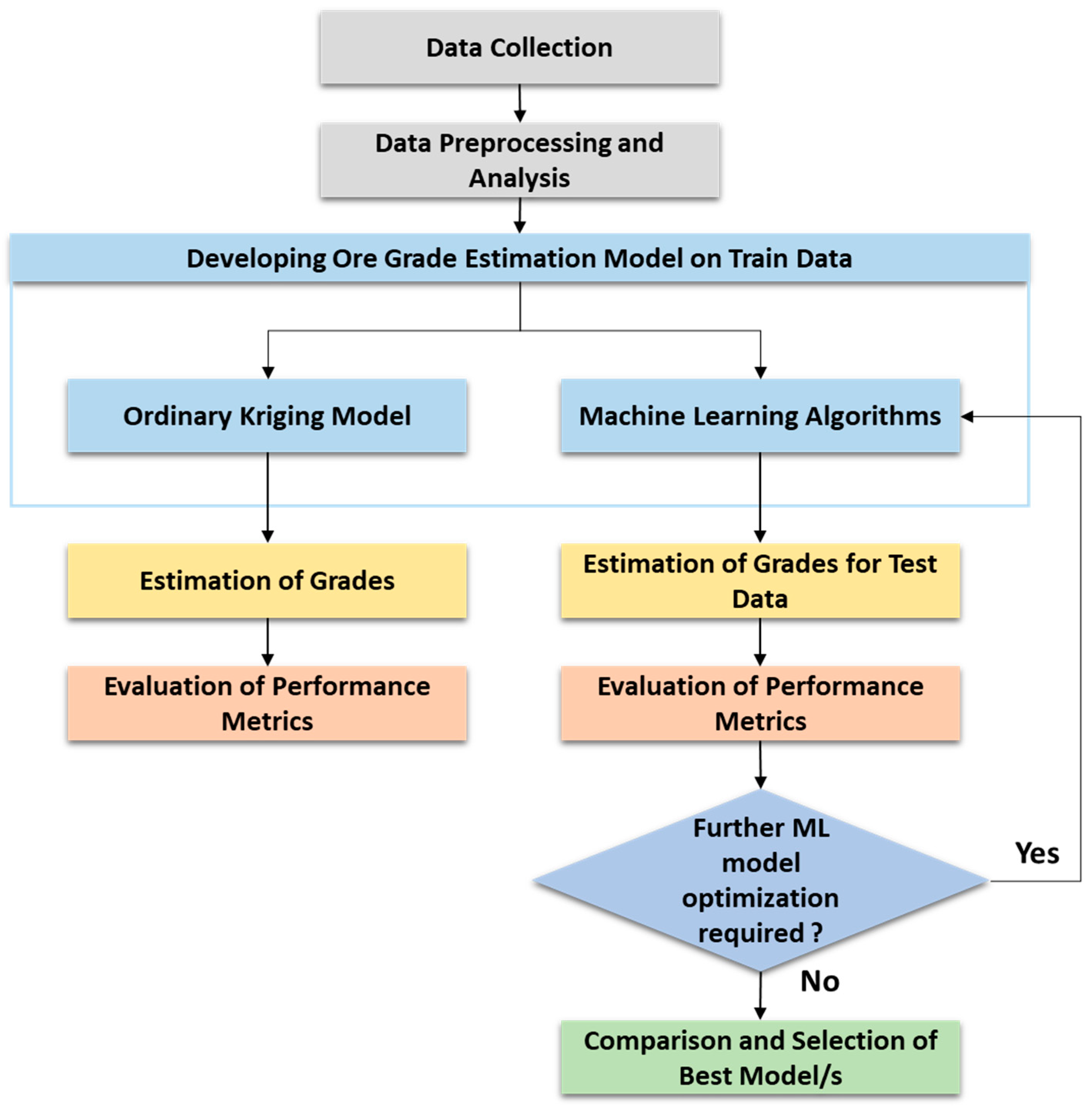
2. Materials and Methods

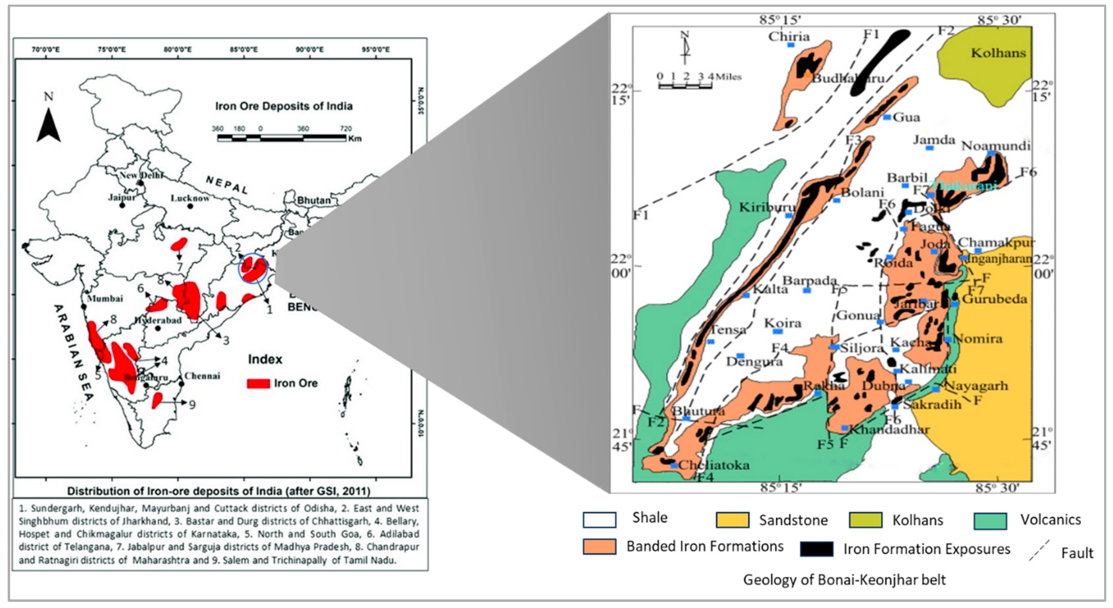
2.1. Geology of the Deposit

The mine is situated in the eastern portion of the Bonai–Keonjhar (BK) belt in the Indian state of Odisha. The BK belt, known for its high-grade hematite iron ore deposits majorly as banded iron formations (BIFs), comprises eastern and western portions. A geological map showing iron ore occurrences in the BK belt is shown in Figure 2. Iron ore bearing and associated rocks of the area are composed of Precambrian sedimentary sequence consisting of variety of iron ore deposits including banded iron formation (BIF), banded hematite jasper (BHJ), detrital iron deposits (DIDs), and brecciated iron deposits (BIDs) [37]. Hematite, magnetite, martite, and specularite are among the iron minerals of oxide facies that make up these minerals. Silica can be found in the form of quartz, jasper, and chert. The overall structural arrangement of the region’s strata is attested by a synclinorium pattern that tends NNE SSE with a low drop towards NNE. The deposit occurs within BHJ on the northern, western, and southern sides, while, on the eastern side, it is mostly covered with laterite.

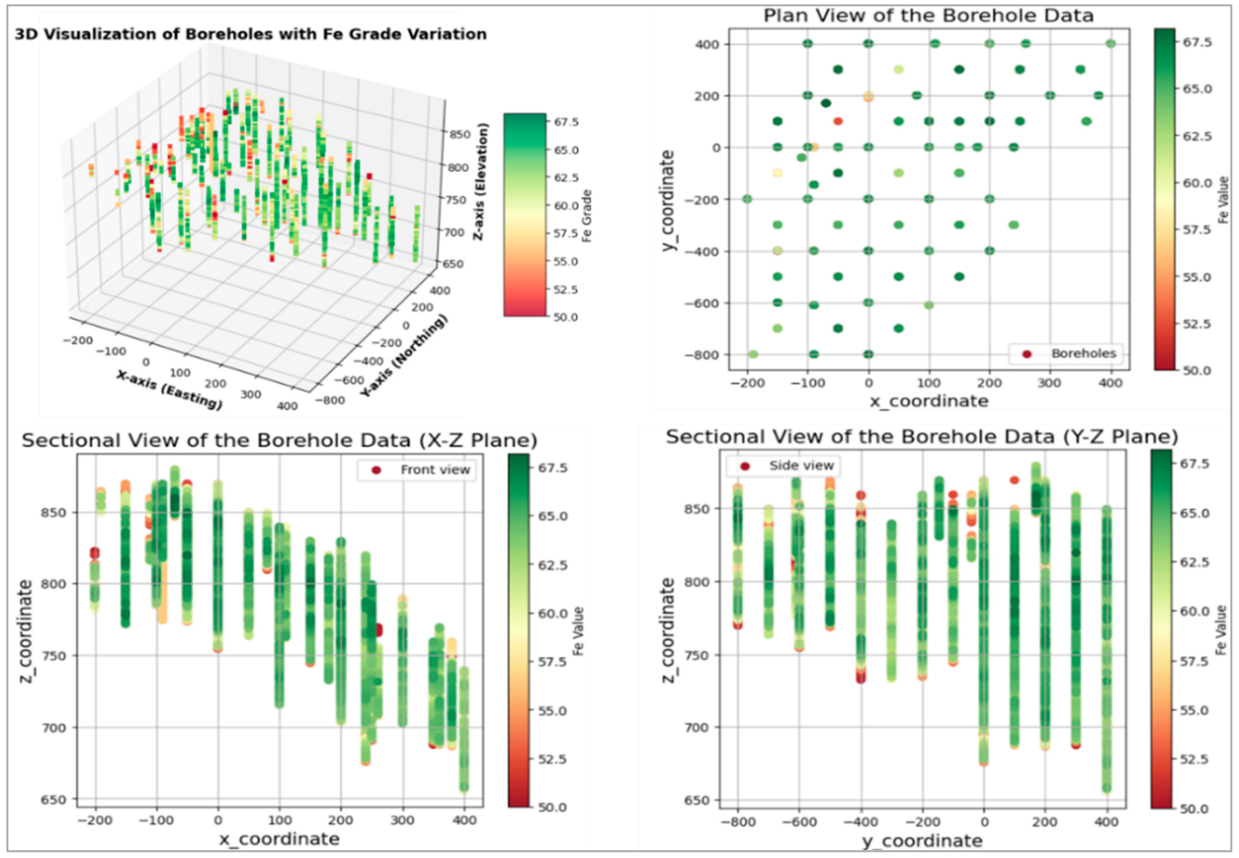
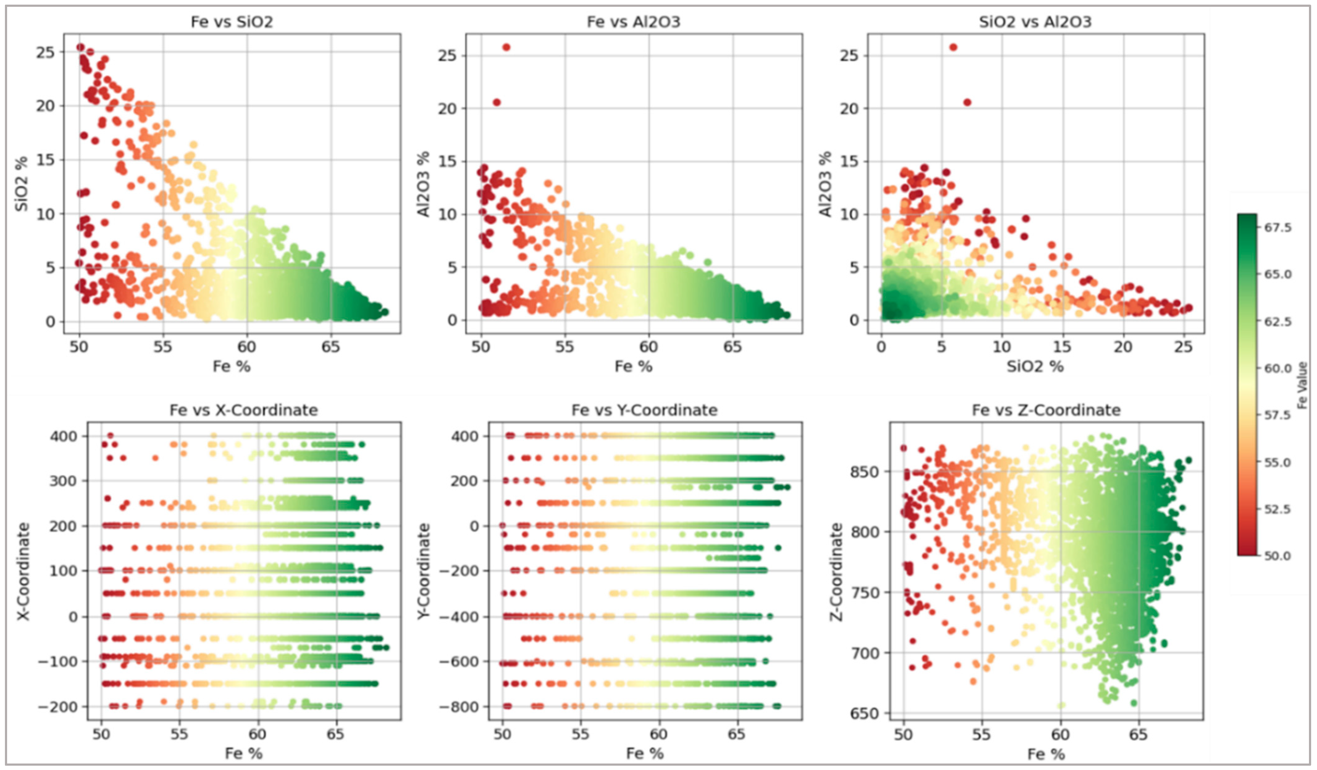
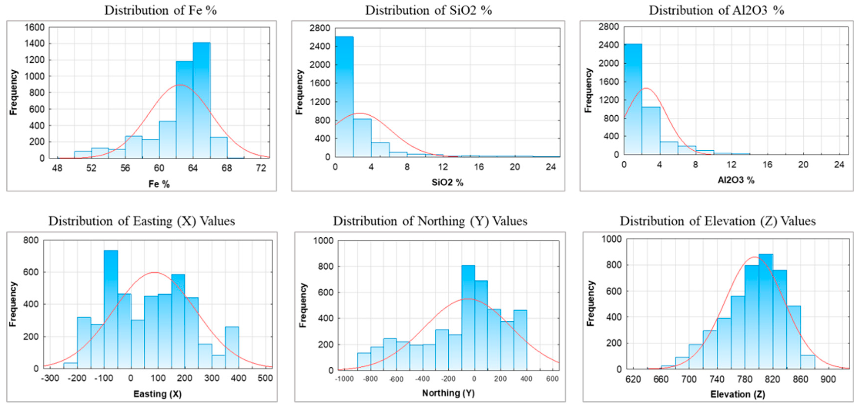
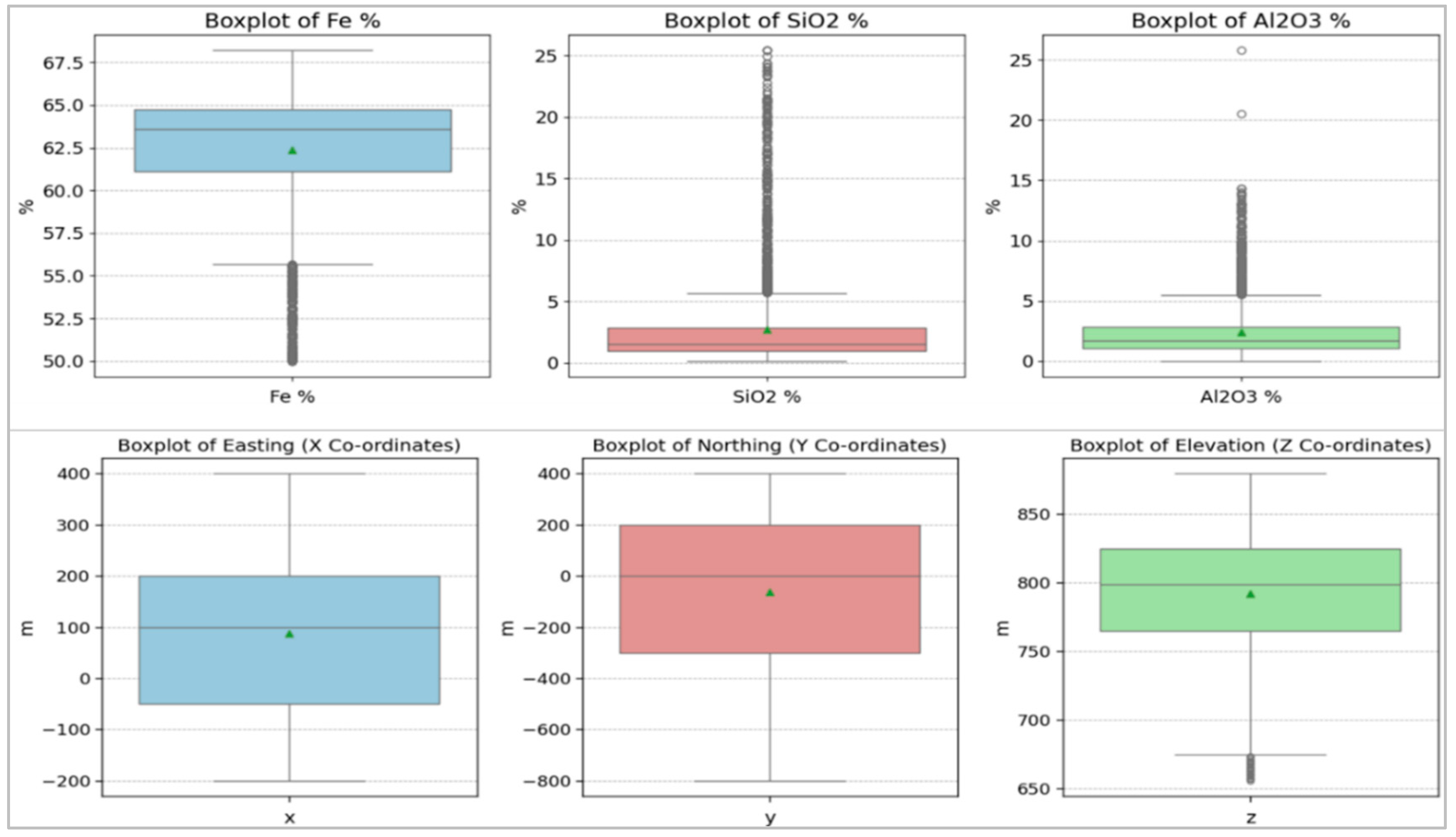
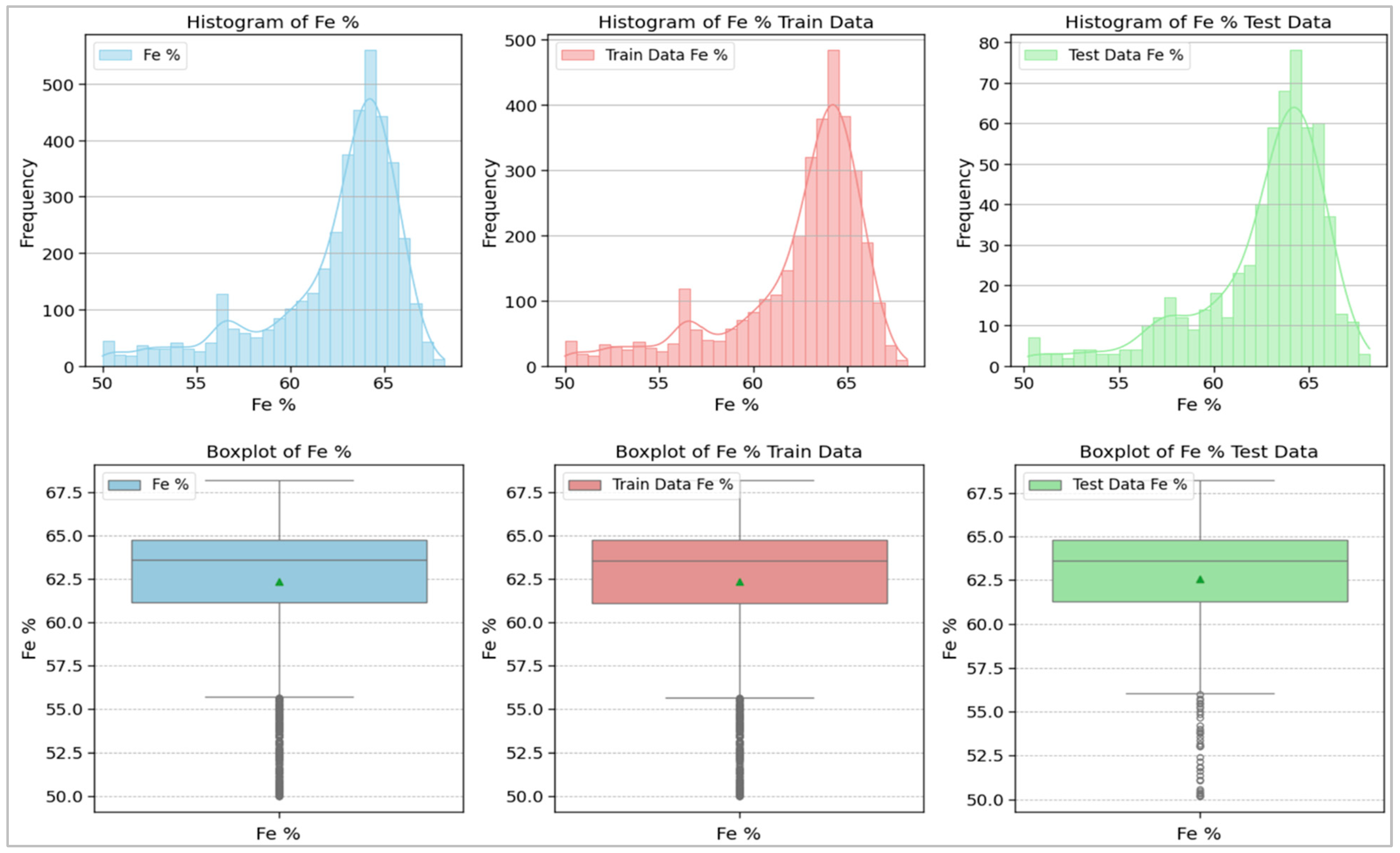
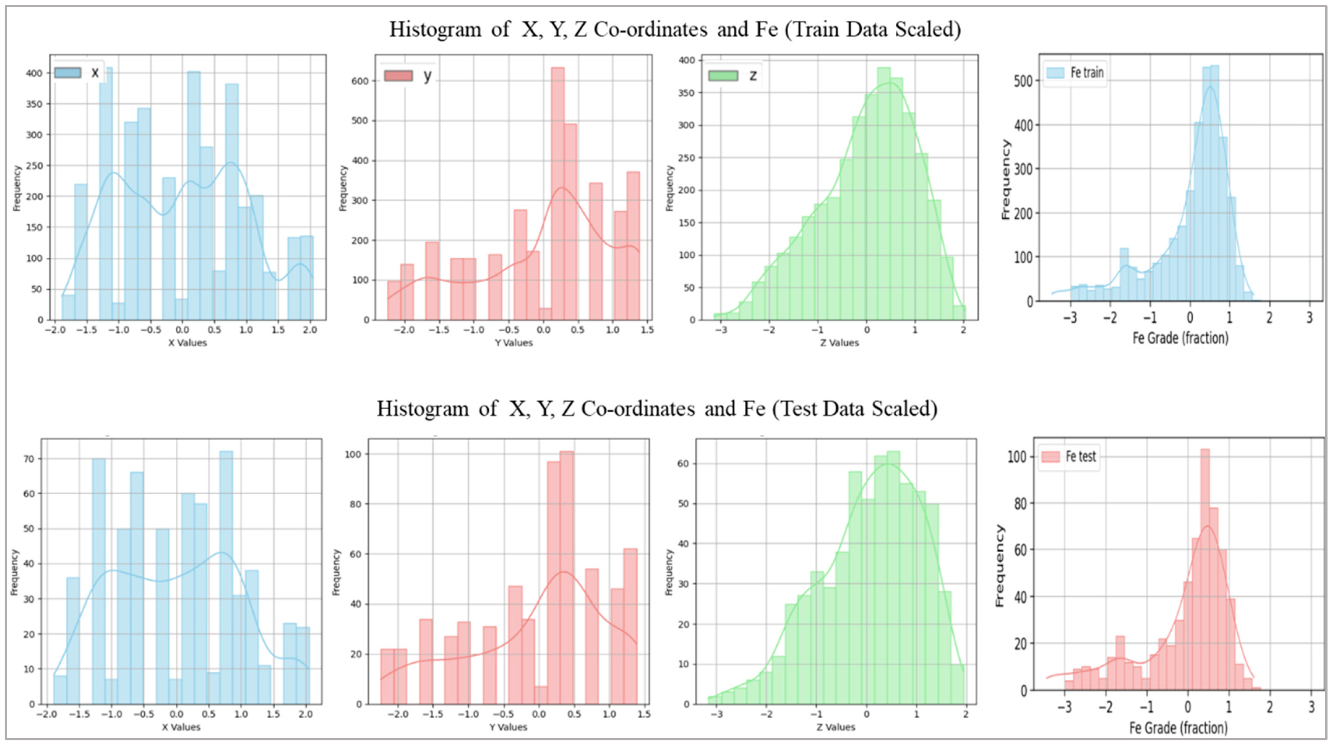
2.2. Data Collection, Preprocessing, and Analysis

For this study, exploratory borehole data are collected for an iron ore deposit. Figure 3 shows the plan and sectional views of the boreholes. The data include 71 boreholes with combined length of 4519 m. The depth of the borehole varies from 7 m to 125 m with an average of 63 m. The drillhole samples are composited at 1 m vertical interval. A geological database is prepared including survey, collar, and assay data. Although the cut-off grade for Fe is 45% as per [40], a threshold value of 50% is used to capture the natural grade variation in the ML model. This resulted in total of 4112 composite sample data points representing 93.88% of the total composite samples generated. Table 1 presents the final geological database that resulted from the data collection process. The database contains information of local spatial coordinates, i.e., easting (X), northing (Y), elevation (Z), and the composition of iron ore (Fe), silica (SiO2), and alumina (Al2O3).
To understand the relationship of iron ore grade, Fe, with other features in the geological database, 2D scatter plots were plotted with colourmap based on grade of Fe as shown in Figure 4. The scatter plots between SiO2, Al2O3, and Fe depicts the inverse relationship of Fe with other two features. The combined effect of SiO2 and Al2O3 on the Fe values also confirms this behaviour. However, the 2D scatter plots between Fe and special coordinates (x, y, and z) does not show any direct linear relationship.
Data visualization through histograms and box plots as shown in Figure 5 were plotted to understand the distribution of the features. Distributions of Fe, Northing (y), and Elevation (z) are negatively skewed, while SiO2, Al2O3, and Easting (x) are positively skewed. The descriptive statistics as shown in Table 2 also reveal distinct patterns and characteristics for each feature in the dataset. Distribution of Fe is negatively skewed with moderately leptokurtic type having mean grade of 62.36% and standard deviation of 3.66%. The high kurtosis values of SiO2 and Al2O3 reveal that the distributions are highly leptokurtic and are positively skewed. The relatively high standard deviations of both the features relative to mean values suggest variability due to heterogenous rock composition. The Anderson–Darling test further confirms the non-normality of the features Fe, SiO2, and Al2O3.
The minimum and maximum of spatial coordinates, i.e., Northing, Easting, and Elevation, are [–800, 400], [–200, 400], and [655.5, 879], respectively. The spatial features show minimal skewness and kurtosis, implying relatively symmetric distributions. However, the lower p-value < 0.05 of Anderson–Darling results indicate non-normality of these distributions.
In modelling iron ore grade estimation using ML algorithms and ordinary kriging (OK), the spatial coordinates (Northing, Easting, and Elevation—x, y, and z) are used as input variable and the iron composition, Fe, is considered as output variable.
Most machine-learning models require data normalization to improve convergence and accuracy, especially when features have varying ranges. Normalization helps in faster convergence and accuracy of the machine-learning models when dealing with features having different ranges [41,42]. In this study, we applied z-score normalization using the StandardScaler method from scikit-learn to standardize the input features. This method transforms the data to an approximate mean of 0 and a standard deviation of 1. The normalization formula is given by Equation (1)
Z = X u s
where Z is the normalized value, X is the original feature value, u is the mean of the feature, and s is the standard deviation of the feature. The normalization was applied to all features for consistency across the preprocessing pipeline, even for models like XGBoost and KNN, which do not strictly require normalization. For models such as support vector regression (SVR), random forest regressor (RFR), and gradient boosting, normalization is critical as these models are sensitive to feature scaling.
Before normalizing the data, splitting operation is performed to create the training and test sets for both input and output features. Data splitting ensures that the test data accurately reflects the real-world scenario and that there is no data leakage [43]. Data splitting is carried out by randomly considering all boreholes using the train test split function of scikit-learn. The splitting operation is performed statistically, ensuring both the train and test sets are representative of the original data. The OK and ML models are developed using the training set, and their performance is assessed using the test data. Of the total 4112 composited sample points, 85% is split into training set and the remaining 15% is used as test set. Train–Test splits are performed statistically, ensuring that the samples are properly representative of the population data, which is confirmed by descriptive statistics and two-sample Z-test hypotheses testing as shown in Table 3. The p-value of the hypothesis testing is > 0.05, suggesting that the train and test splits are consistent with the original data.
Figure 6 shows the histogram and boxplots of Fe for original, train, and test data. The distributions of the splits are comparable to original dataset, meaning that train and test splits are statistically similar to that of original data.
Post-splitting, the features are then normalized to standard distribution with mean ≈ 0 and SD ≈ 1 as shown in Figure 7 and Table 4. The normalized train and test data are then used for training and evaluation of the ore grade estimation models, respectively.

3. Ore Grade Estimation Models

Ore grade estimation models are developed using ML techniques. The results are compared with standard ordinary kriging model. The underlying concept of machine learning (ML) is different from such geostatistical techniques as ordinary kriging in providing spatial predictions. Geostatistical models work on the basis of the spatial geological continuity of the deposit. The spatial continuity is captured using variogram modelling. This is used in the estimation by the kriging method. This enables geostatistical methods to include spatial continuity in the estimation directly.
On the other hand, ML algorithms are not innately equipped with a way to quantify or use geological continuity in a similar manner. Instead, they rely on the training data, which contains spatial coordinates among other predictor variables, to learn patterns from the data. Although this method can provide relatively accurate predictions in many cases, it does not necessarily model spatial continuity in the same way as geostatistical methods. This differentiates a fundamental variation between geostatistical and ML methods.
In this study, four machine-learning models and an ordinary kriging model have been developed to estimate the iron ore grade.

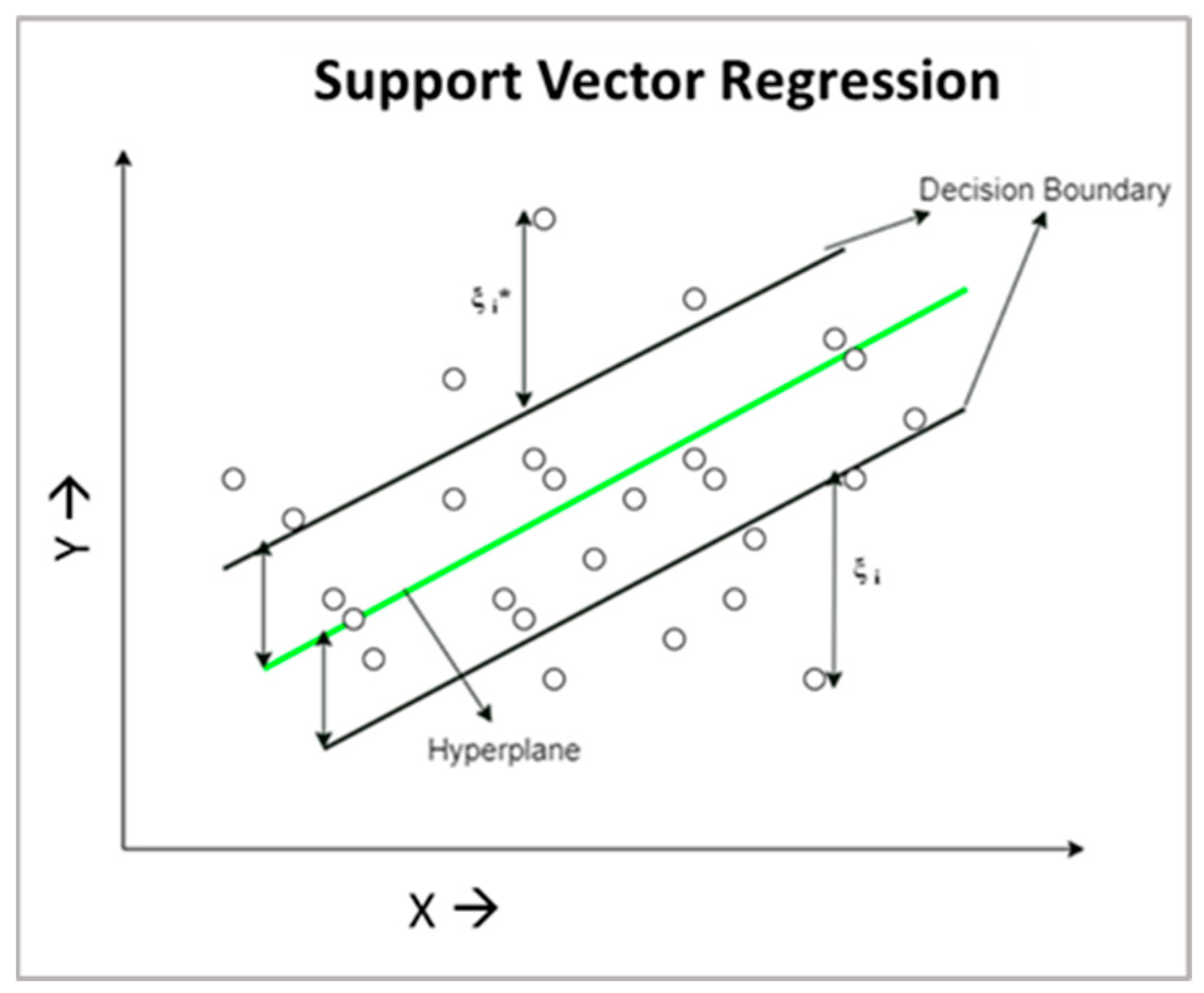
3.1. Support Vector Regression (SVR)

SVR is a regression problem extension of the support vector machine (SVM) classification model. To generalize the SVM to SVR, an insensitive zone known as the ε-tube is added around the function [44]. A non-linear kernel function is used to convert input features from the original space into a higher dimension. The problem becomes the construction of an optimal linear surface that matches the data in the feature space [45]. To find the ε-tube that optimizes the model while balancing its complexity and prediction error, the optimization problem is rewritten based on this insensitive zone. The mathematical equation of SVR model is given by Equation (2)
Y = f ( X ) = W o T     Ø X + b
where X and Y are the input and output random variables; W 0 is the optimum weight vector; Ø ( X ) refers to the kernel function that transforms the input variable from the input space to a feature space of a higher dimension; and b is the bias. The radial basis function (rbf), and polynomial, linear, and sigmoid tanh functions are among the different kernel functions. Rbf is the most popularly used kernel function and is defined by Equation (3). The key hyperparameters of the SVR model C, γ, and ε are to be optimized for a better model output [46,47].
K x i , x = e x p ( γ   x x i 2 )
The errors are measured from the closest edge for those points lying outside the insensitive tube (ξ) as shown in Figure 8. The points above the tube are denoted by ξ i * and the points below are denoted by ξ i . The solution to the SVR optimization is obtained by minimizing the loss function, which is given by Equation (4) subject to the constraints in Equation (5)
L = min w 2 + C   i = 1 N | ξ i |
subject to the following constraints:
y i y ^ i = y i W o T     Ø X + b   ε + ξ i
y ^ i y i = W o T     Ø X + b y i   ε + ξ i *   ;     ξ i , ξ i * 0
Solving the minimization equation yields an optimal hyperplane (Figure 8) whose equation is defined as per Equation (6):
y ^ i = i = 1 N ( α i α i * ) Ø x i Ø x + b
y ^ i = i = 1 N ( α i α i * ) K x i , x + b  
Here, α i , α i * are called the dual coefficients, and they are upper-bounded by C which refers to the regularization parameter; and K x i , x refers to the kernel function.

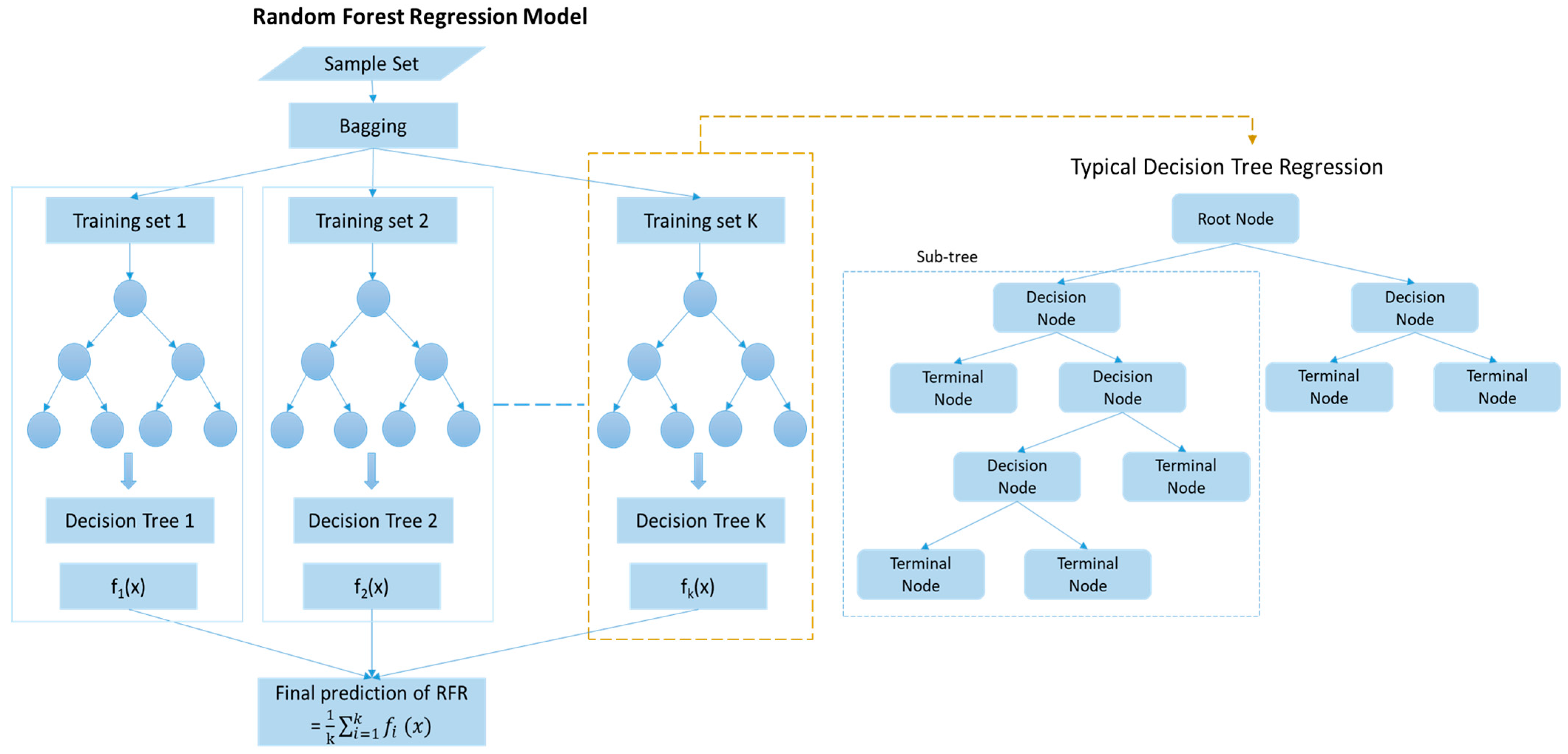
3.2. Random Forest Regression (RFR)

RFR is a meta estimator that fits multiple classification decision trees on various dataset sub-samples using averaging to increase the predicted accuracy while controlling over-fitting. It is an ensemble technique where several outputs are combined to give a final output, hence the name forest. Random samples are generated from the original data using “Bootstrap Aggregating” (also referred to as bagging). Bagging is a random sampling method which creates samples with replacement [48,49,50,51,52].
In the RFR model, for a given group of training data containing N observations, several random samples, Si, of size M (M < N) are generated using the bagging technique. Overall, K models are developed as shown in Figure 9, where K refers to the number of decision tree regression (DTR) models to be used. For each sample Si generated, a decision tree (DT) is developed, and a result ( f i ) is predicted. Once predictions are made for all the DTR models, the average of all DTs is calculated using Equation (7) to predict the output of the RFR.
ŷ = 1 K i = 1 K f i
Here, K refers to the number of DTs; f i is the prediction of the ith DT; and ŷ is output of the RFR model. The concept used here is that, while individual DT estimates may be less accurate in forecasting target values, the average of the predictions of several DTs will converge to the actual target value [53]. The working of a decision tree is explained by [54,55]. Various hyperparameters of the RFR model include the number of decision trees, the maximum depth of the DT, the minimum samples in each leaf, etc. Hence, the RFR model requires hyperparameter tuning to find the best-fit model.

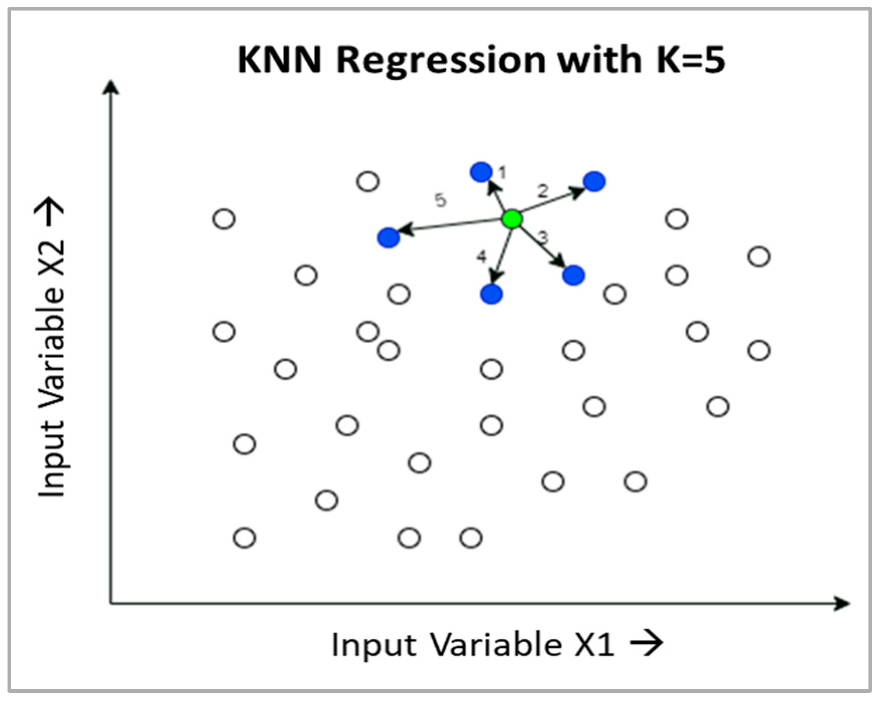
3.3. K-Nearest Neighbour (KNN) Regression

KNN regression is a non-parametric algorithm that predicts outcomes based on the proximity and density of neighbouring data points. It is particularly useful when the nearby points have a significant impact, such as in geospatial data predictions. The value ‘k’ is a user-defined parameter which refers to the number of neighbouring points that have an influence on the prediction point. The model assigns weights to these points based on the Euclidean distance. The closest points have the highest weights and vice versa [56]. The distance between two points x 1 ,   y 1 and x 2 ,   y 2 is calculated as per Equation (8).
E u c l i d e a n   d i s t a n c e ,   d = { y 1 y 2 2 x 1 x 2 2 }
The KNN regression returns the prediction value by calculating the weighted average of the nearest points. Hence, the distance between points is crucial, as the model gives more weight to nearer neighbours. The method is useful for a variety of data types, especially when the location of data points plays a role in predictions [57,58].
To find the nearest neighbours efficiently, algorithms like Brute Force, KD Tree, and Ball Tree are employed. Brute Force compares all pairs of points but is computationally heavy with larger datasets. The KD Tree algorithm improves efficiency by organizing the data in a binary tree, reducing the computational load, but suffers from performance in higher dimensions (>20). The Ball Tree algorithm is effective as it organizes data in nested hyper-spheres, allowing for quick searches even in high-dimensional space [59]. Figure 10 shows the identification of neighbours in a typical KNN regression when k = 5.

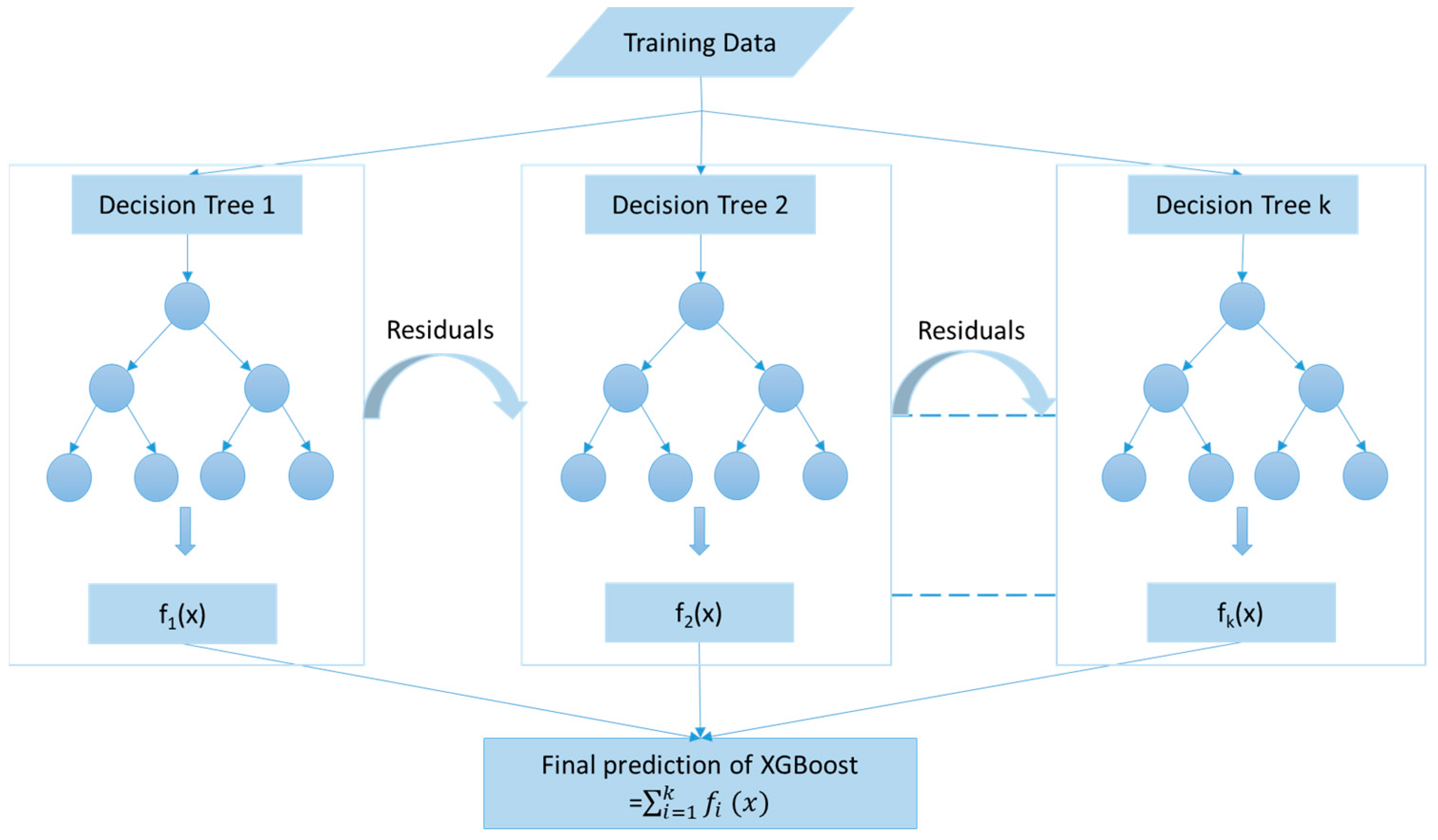
3.4. XGBoost Regression

The extreme gradient boosting, or XGBoost, regression is a powerful machine-learning regression technique based on gradient-boosting principles, with speed and accuracy advancements [60]. With its integrated regularization, XGBoost is a powerful algorithm that can handle intricate datasets and minimize overfitting. The method optimizes model predictions by sequentially adding decision trees that reduce the residuals of previous models, using second-order gradient information for improved precision [61]. Minimizing a regularized objective function after several iterations is the fundamental concept of XGBoost. Given a dataset D =   x i ,   y i i = 1 n , where x i represents the input features and y i the target feature, the regularized objective is defined as per Equation (9).
L θ = i = 1 n l y i ,   y ^ i + k = 1 K Ω f k
Here, l is the loss function which is calculated as l y i ,   y ^ i = y i y ^ 2 , y ^ i is the predicted target output, f k represents an arbitrary tree among K trees, and Ω f k is the regularization term to prevent the overfitting of the model [62]. The regularization term is expressed as per Equation (10)
Ω f k = γ T + 1 2 λ   j = 1 T w j 2
where T refers to the boosting tree’s leaf count, w j denotes the weights of the leaf, and γ and λ are L1 and L2 regularization parameters. As seen in Figure 11, with the objective of reducing the errors of the previous tree, the trees are built one after the other. Consequently, the tree that grows next in the sequence will be modeled using an updated version of the residuals. The main hyperparameters of XGBoost regression include the learning rate (η), which regulates each tree’s contribution; max_depth, which limits the depth of the trees to reduce overfitting; and n_estimators, which represents the number of trees [63].

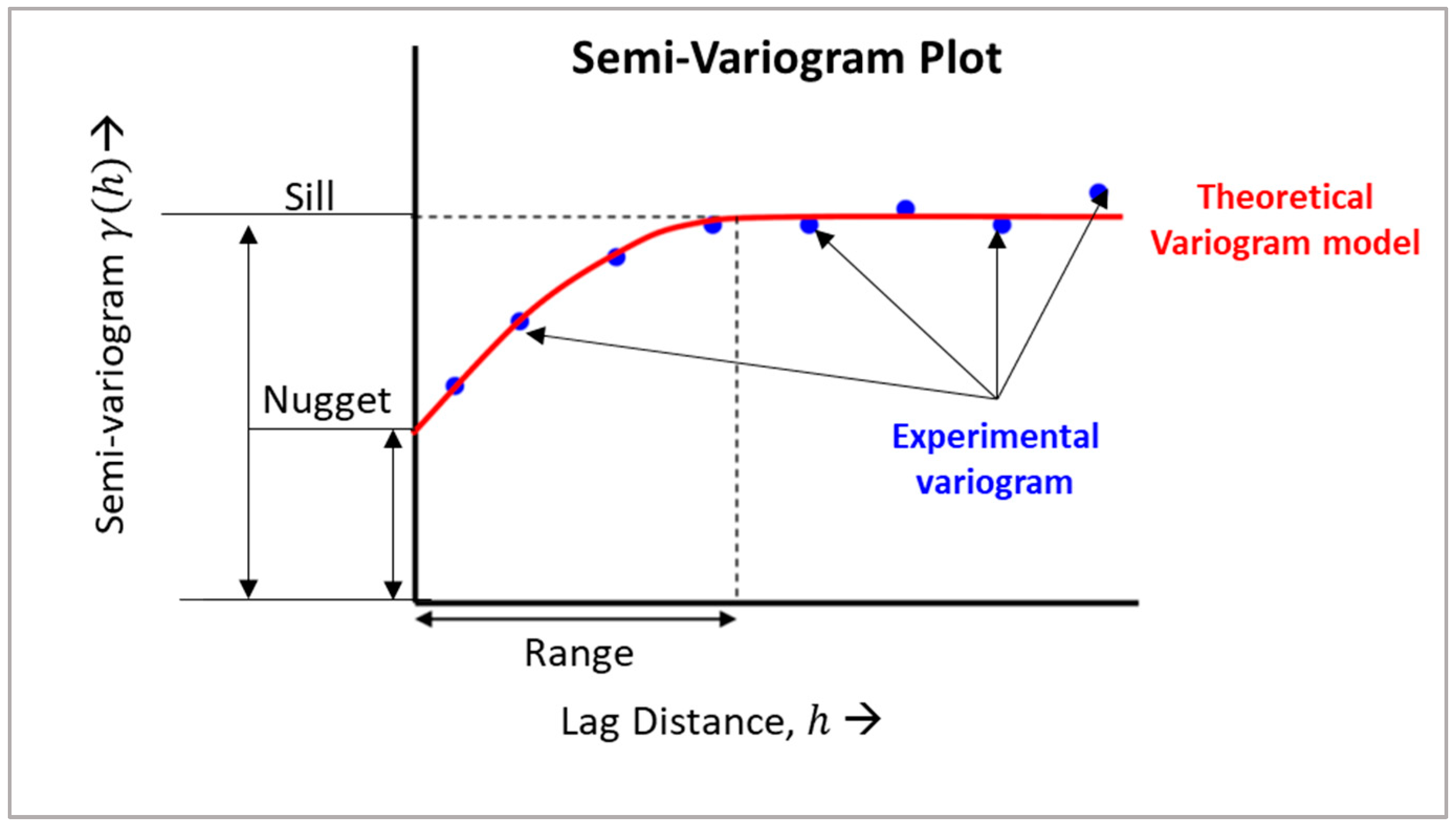
3.5. Geostatistical Ordinary Kriging Method

Geostatistical estimation models involve three major steps, i.e., understanding the spatial continuity, variogram modelling, and kriging estimation. Spatial continuity is the correlation between values over distance in space and is usually observed by scatter or h-scatter plots. A semi-variogram quantifies the deposit’s spatial continuity. It is calculated by Equation (11)
γ h = 1 2 N h i = 1 N ( h ) Z ( u i ) Z ( u i + h ) 2  
where γ(h) represents the semi-variogram value, Z ( u ) is the grade value at point u , h is the lag distance between two points, and N (h) represents the total number of points that can be separated by a lag distance h . Using this, an experimental semi-variogram is plotted and a theoretical variogram model such as a spherical model, Gaussian model, exponential model, etc. is best fitted on the experimental variogram for a smooth continuous curve [65]. A typical semi-variogram plot is depicted in Figure 12. The output elements of the semi-variogram include the sill, nugget, and range.
Ordinary kriging (OK) is a geostatistical technique that uses semi-variogram inferences to estimate grades at an unknown location. By restricting the domain of mean stationarity to neighbourhood samples, the OK approach incorporates the local mean variation under consideration [65]. OK eliminates the requirement for the knowledge of the mean by necessitating global impartiality, which limits the sum of the weights to 1.0. The unique feature of kriging is that it not only calculates an estimate of the variable but also gives the estimation variance at each interpolated point, therefore providing a measure of confidence in the modelled surface [66]. The estimation and minimum variance by OK are expressed by Equations (12) and (13)
Z * u 0 = i = 1 n λ i . Z u i ;     i = 1 n λ i = 1
σ u 0 2 = i = 1 n λ i     γ u i , u o + μ
where Z * u 0 is the predicted grade at unknown location u 0 , σ u 0 2 is the variance of estimation at u 0 , [ λ ] are the weights of the linear kriging equation which are derived using the variogram model, μ is the Lagrange multiplier, γ u i , u o is the covariance between estimations at u i and u 0 , and γ u i , u 0 is the variogram between estimations at u i and u 0 .

4. Results and Discussion

The ore grade estimation models developed include the SVM, RFR, KNN, XGBoost regression, and OK model. Table 5 shows the details of the hyperparameters used for developing the models and the optimal design results. The ML models were developed using the open-source Python packages scikit-learn, pykrige, and skgstat. The hyperparameters are tuned using the RandomizedSearchCV method with the number of estimators set at 95% of the possible hyperparameter combinations. All the models were developed using training data, which represent 85% of the total data, and their performance were tested using a test set, which consists of remaining 15% data. Statistical performance metrics including R2, RMSE, and MAE were computed for the training and test sets using the Equations (14)–(16), respectively. Additionally, scatter plots, residual histograms, and residual plots were charted out to visualize the results.
R 2 = 1 i = 1 N y i y ^ i 2 i = 1 N y i y ¯ i 2
M S E = 1 N i = 1 N y i y ^ i 2
M A E = 1 N i = 1 N | y i y ^ i |

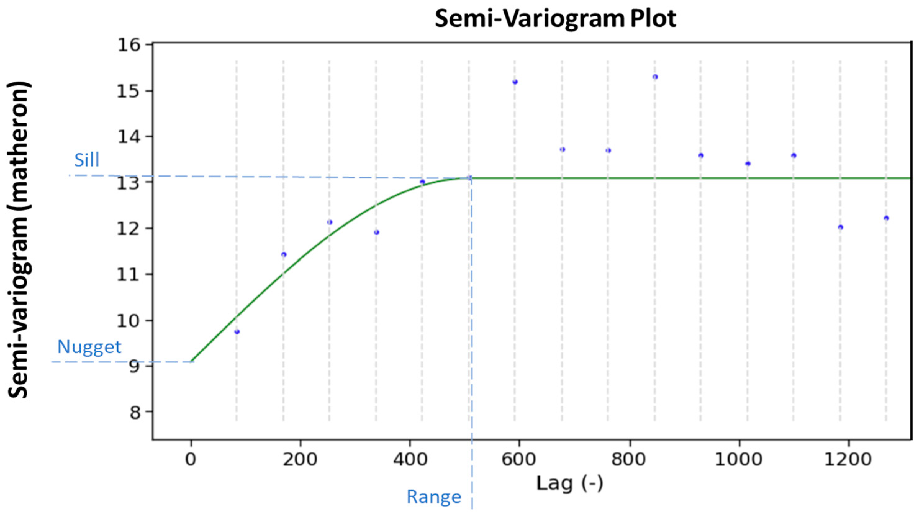
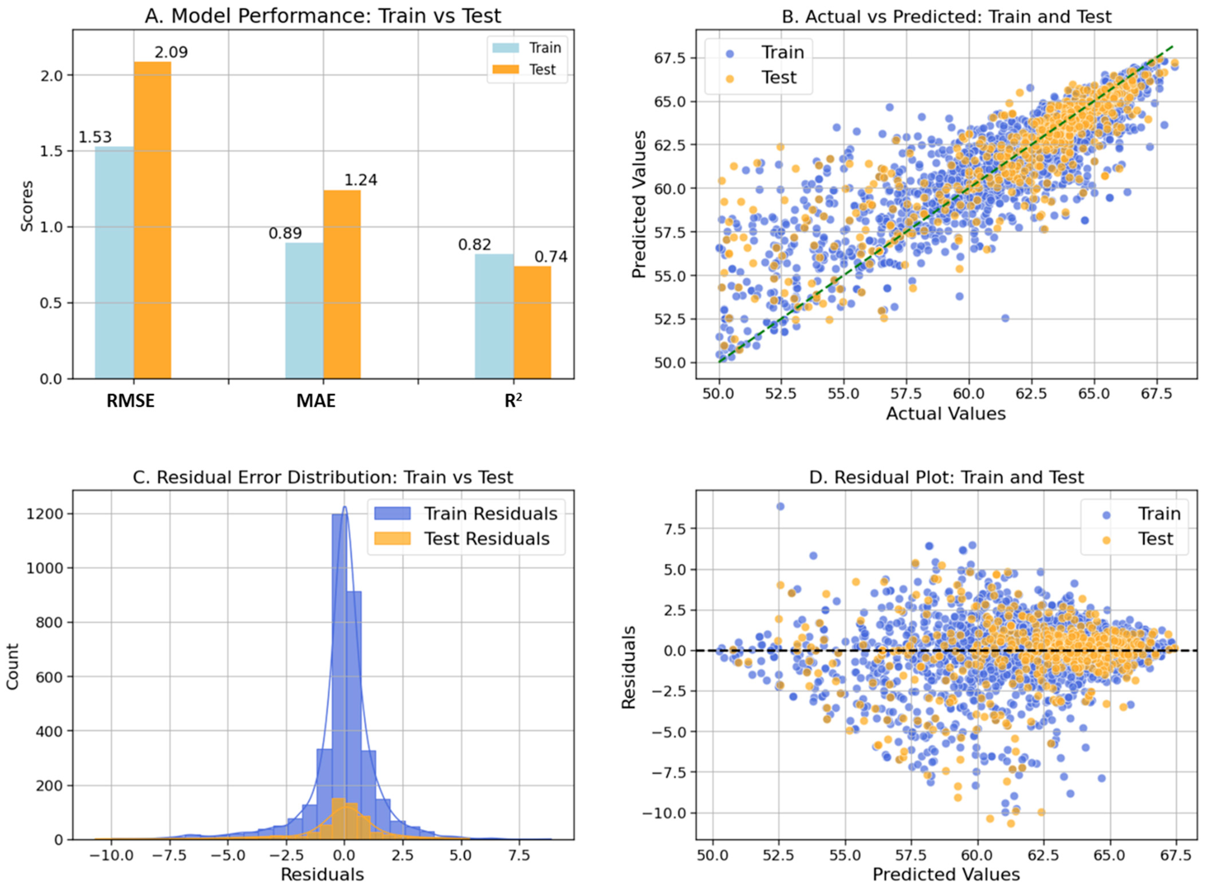
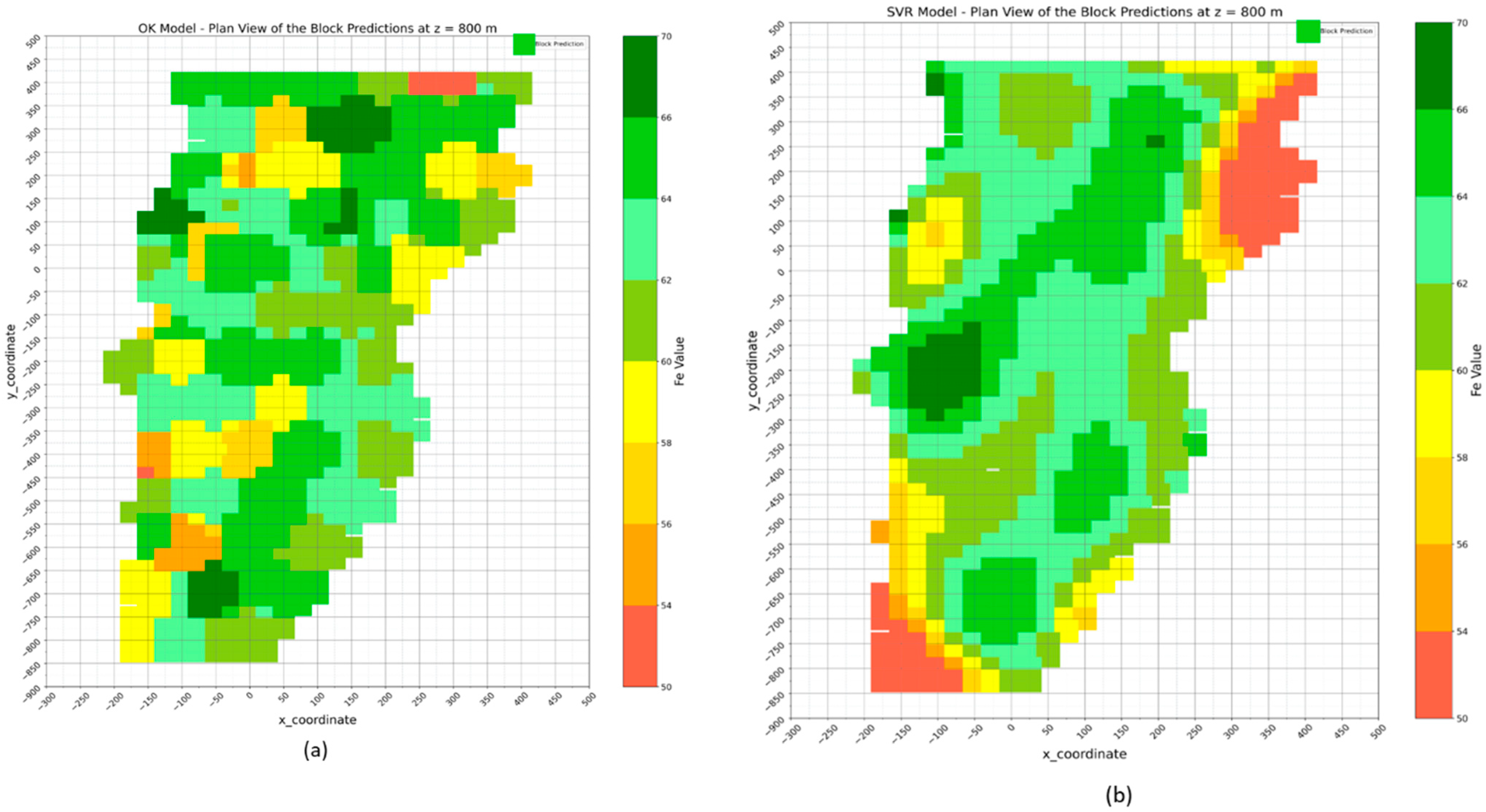
4.1. Geostatistical Ordinary Kriging Model

Ordinary kriging (OK) was developed and used as the standard geostatistical ore grade estimation method to compare the machine-learning model estimation results. The variogram modelling and kriging estimates are executed in Python using the gstools and scikit learn geostatisics libraries. Directional semi-variograms for this deposit could not produce any discernible pattern of anisotropy in the spatial continuity. Therefore, an omnidirectional semi-variogram was developed as shown in Figure 13. The experimental variogram is fitted with a spherical model showing a fitness Pearson’s coefficient of 0.85. The fitted spherical semi-variogram model shows a nugget effect of 9.08 (%)2, and a sill value of 13.08 (%)2, with a range of influence of 508.4 m.
The OK model was used to estimate the Fe grades at test data locations. Figure 14 shows the results of the OK model. Despite being the standard method, OK showed an R2 of 0.82 for the train dataset and 0.73 for the test dataset. The RMSE for the train and test data stood at 1.53 and 2.09, respectively. The model predicted higher grade values of Fe than the actual values on the lower range which is apparent as shown in the Figure 14B scatter plot. The residuals (i.e., actual value—predicted value) shown in the residual plot also illustrates this with higher negative values scattered around 55–62% Fe.
Ordinary kriging (OK) relies heavily on variogram parameters, which define the spatial structure of the dataset. In this study, the fitted spherical variogram model was characterized by a nugget of 9.08 (%)2, a sill of 13.07 (%)2, and a range of 508.5 m. The moderate nugget effect indicates short-range variability or measurement errors, reducing OK’s ability to predict localized Fe grade variations accurately. The range of 508.5 m suggests that the spatial correlation diminishes beyond this distance, particularly impacting prediction reliability in sparsely sampled regions. Furthermore, the stationarity assumption of the kriging method and the dependency on the best fit of the theoretical model on the experimental model (in this case, the spherical model) could be plausible reasons for the R2 of 0.74.

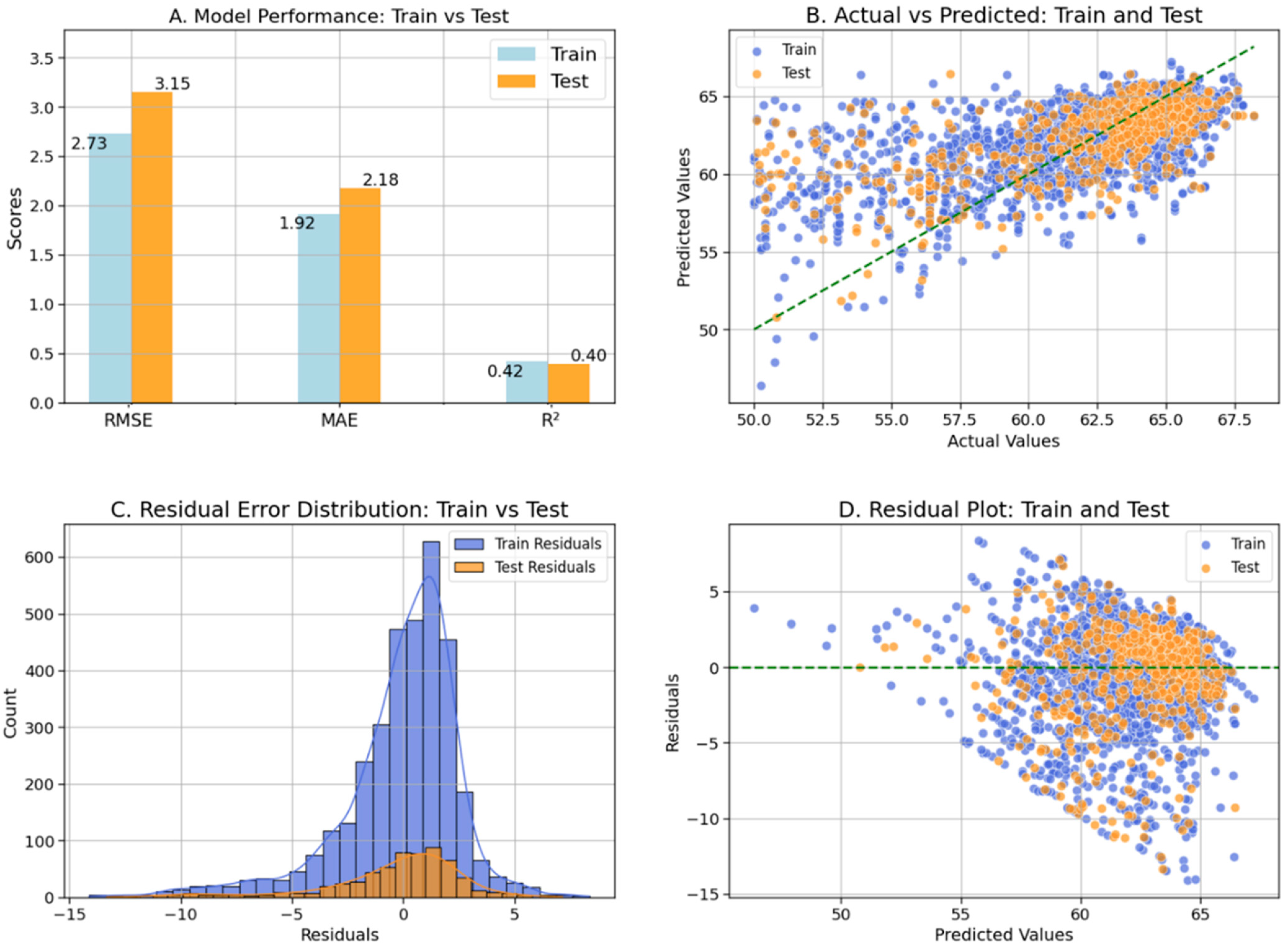
4.2. Support Vector Regression (SVR) Model

The SVR model was optimized using the hyperparameters as shown in Table 5 and found the optimal values as C = 500, epsilon, gamma, kernel, and the degree for the polynomial kernel. The SVR model, despite an extensive hyperparameter search, exhibited weaker performance, as shown in Figure 15. The R2 values were also low, with 0.42 and 0.40 for the train and test sets, respectively, suggesting that SVR struggles to capture the variance in the dataset effectively. Similarly, the higher values of the RMSE of 2.73 and 3.15, and MAE of 1.92 and 2.18 for the train and test datasets, respectively, indicate a poor fit. In the actual vs. predicted plot (Figure 15B), the wide dispersion of the predicted values around the diagonal line further underscores SVR’s difficulty in predicting the iron ore grade. The errors were substantial, with both the training and test data showing significant deviations from the actual values. The residual distribution (Figure 15C) and residual plot (Figure 15D) reflect a similar pattern. This is likely due to the limitations of SVR in handling complex, non-linear relationships present in this geological database. The lack of a clear pattern in the residuals suggests that the model is not overfitting but is simply underperforming in modeling the underlying relationships between the spatial coordinates and iron ore grade. The complexity of the dataset likely required a more flexible model, and, based on these results, SVR was the least effective among the models tested.

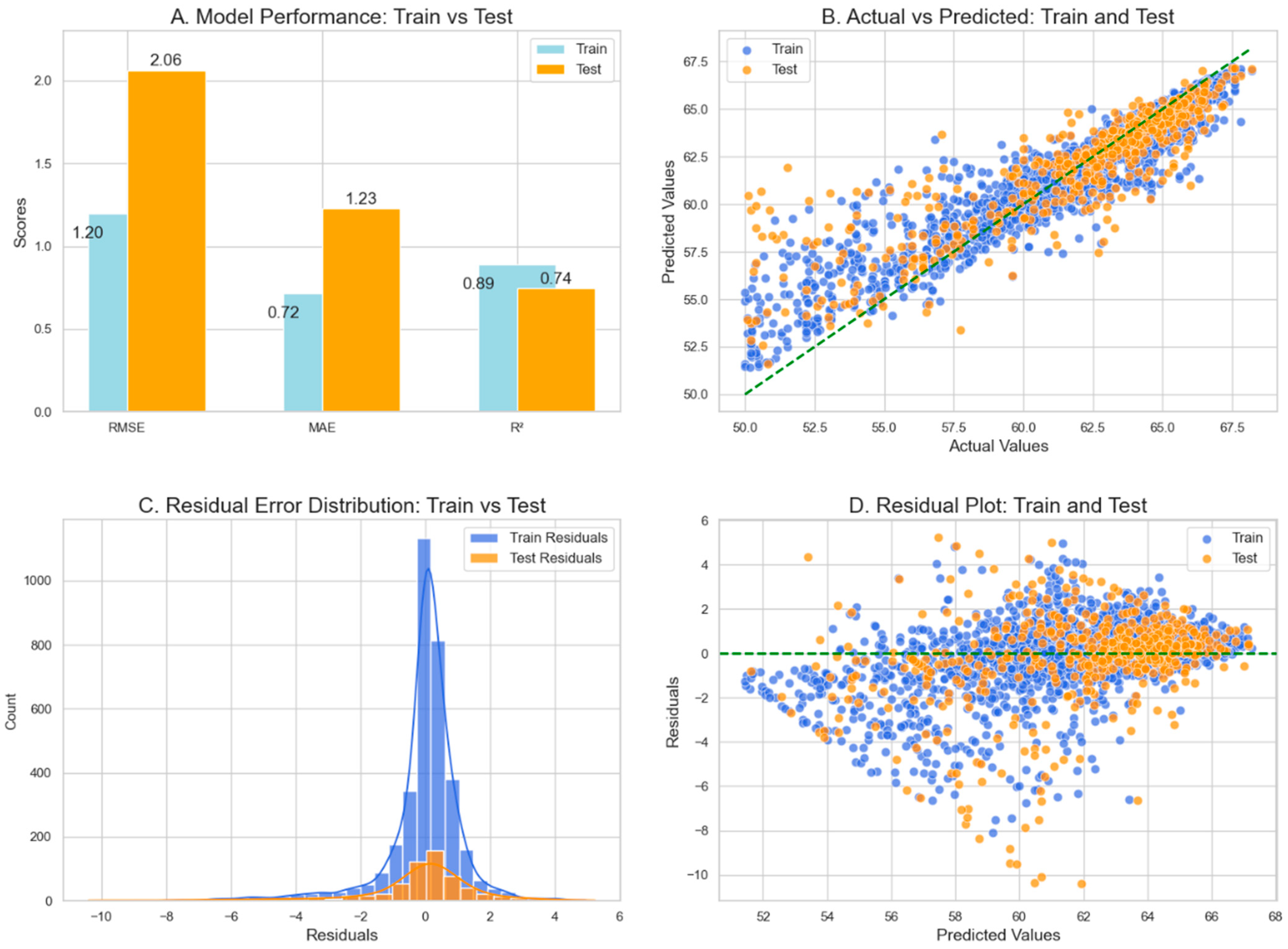
4.3. Random Forest Regressor (RFR) Model

The RFR was developed with the design criteria as described in Table 5, employing RandomizedSearchCV to fine-tune key hyperparameters, including the number of estimators, maximum depth, and minimum samples split. The hyperparameter tuning aimed to balance model complexity and prediction accuracy while preventing overfitting. Figure 16 offers a comprehensive view of the random forest regressor model’s performance. The R2 value, indicating the amount of the explained variation by the regression model, was 0.89 for the training set and 0.74 for the test set. The decline in R2 from the train to the test data indicates that, although the model performed well on the training data, its ability to generalize to the test data was slightly limited, indicating mild overfitting. The lower RMSE values of 1.20 and 2.06 for both the train and test sets, respectively, as compared to their respective standard deviations, suggests the model captures the natural variation of the grade. The MAE values of 0.72 and 1.23 indicates mild overfitting in the model which is acceptable.
The scatter plot in Figure 16B illustrates the correlation between the actual and predicted Fe grades for both the training and test sets. The predictions for the training set (blue) and test set (orange) closely follow the diagonal line, indicating the predictions with minimal error. While the model maintained the consistency between the actuals and predictions on higher grades of Fe (> 60%), it struggled to do the same in lower grade values. It may be attributed to the lower proportion of the lower Fe values in the geological database. The high variability in the residuals plot at lower Fe values further confirms the same.

4.4. K-Nearest Neighbour (KNN) Regression Model

The KNN model was developed using a bagging regressor with key hyperparameters including n_neighbour, leaf_size, n_estimators, max_samples, and distance metric. The optimization with hyperparameter tuning resulted in a good-performing KNN model as shown in Figure 17, having R2 values of 0.82 and 0.73 for the train and test data, respectively. While the predictions for the test set are on the lower side than the train set, the slightly lower difference between the two shows the model did not overfit the data. Overfitting is less than that of RFR.
The RMSE and MAE for the training set are 1.54 and 0.93, respectively, which are relatively lower than the 2.11 and 1.29 for the test set. This indicates that the model has a higher error when predicting on unseen test data, while performing comparatively better on training data. The results suggest that KNN is still an effective method in capturing spatial relationships within the data, achieving the closer generalization capability of the OK model. The actual vs. predicted plot (Figure 17B) shows that the predictions for the training set align closely with the actual values, as data points cluster near the diagonal line. However, data points are more dispersed for both the train and test sets on lower grade values, reflecting its relatively inferior performance in this region. The model could reveal patterns that were not captured by the OK model, suggesting that KNN generalization is better than the former.

4.5. XGBoost Regression Model

The XGBoost model was developed and optimized using the hyperparameters ‘number of estimators’, ‘learning rate’, ‘maximum depth’, ‘min_child_wight’, ‘gamma’, and ‘booster’ type, as listed in Table 5. Figure 18 summarizes the performance of the XGBoost, where the model’s predictions and error distributions are laid out for both the training and test sets.
The XGBoost regression model achieved an RMSE of 1.34 on the training set and 2.12 on the test set, suggesting that, while the model slightly overfits, it generalizes well for both train–test sets. This is further emphasized by the R2 values, where the training R2 is 0.86, but it drops to 0.73 on the test set. The outcome of the model on the test set indicates mild and acceptable levels of overfitting. The MAE values (1.04 for training and 1.47 for testing) indicates that the model captures a majority of the variation of the dataset. The actual vs. predicted plot (Figure 18B) illustrates this trend, with training data points clustering closely around the diagonal, indicating a good fit. However, the test data points are relatively dispersed, which is consistent with the lower performance on the test set.
The residual distribution (Figure 18C) reflects a tight fit around zero for the training set, showing that the model captures most patterns well in the training phase. However, the wider spread of residuals in the test set points to the model deviations with new unseen data. Overall, XGBoost performed well, generalizing closer to that of the KNN, RFR, and OK results.
The strengths and limitations of machine-learning (ML) models are critically evaluated in the context of mining applications, as summarized in Table 6. While ML models offer significant advantages, such as the ability to handle non-linear relationships, flexibility in high-dimensional data, and robustness to noise, they also exhibit notable limitations. A key limitation is the absence of inherent uncertainty quantification, a feature provided by geostatistical methods such as ordinary kriging (OK). This limitation restricts ML models’ utility in risk assessment and decision-making processes that are integral to mining operations.
Another limitation is the site-specific nature of ML models, which are typically developed using data from a single mine site. While this ensures a high predictive accuracy for the target site, it limits the generalizability of the models to other locations. To address these limitations, future work could focus on integrating ML with geostatistical techniques to incorporate uncertainty quantification and enhance model adaptability.

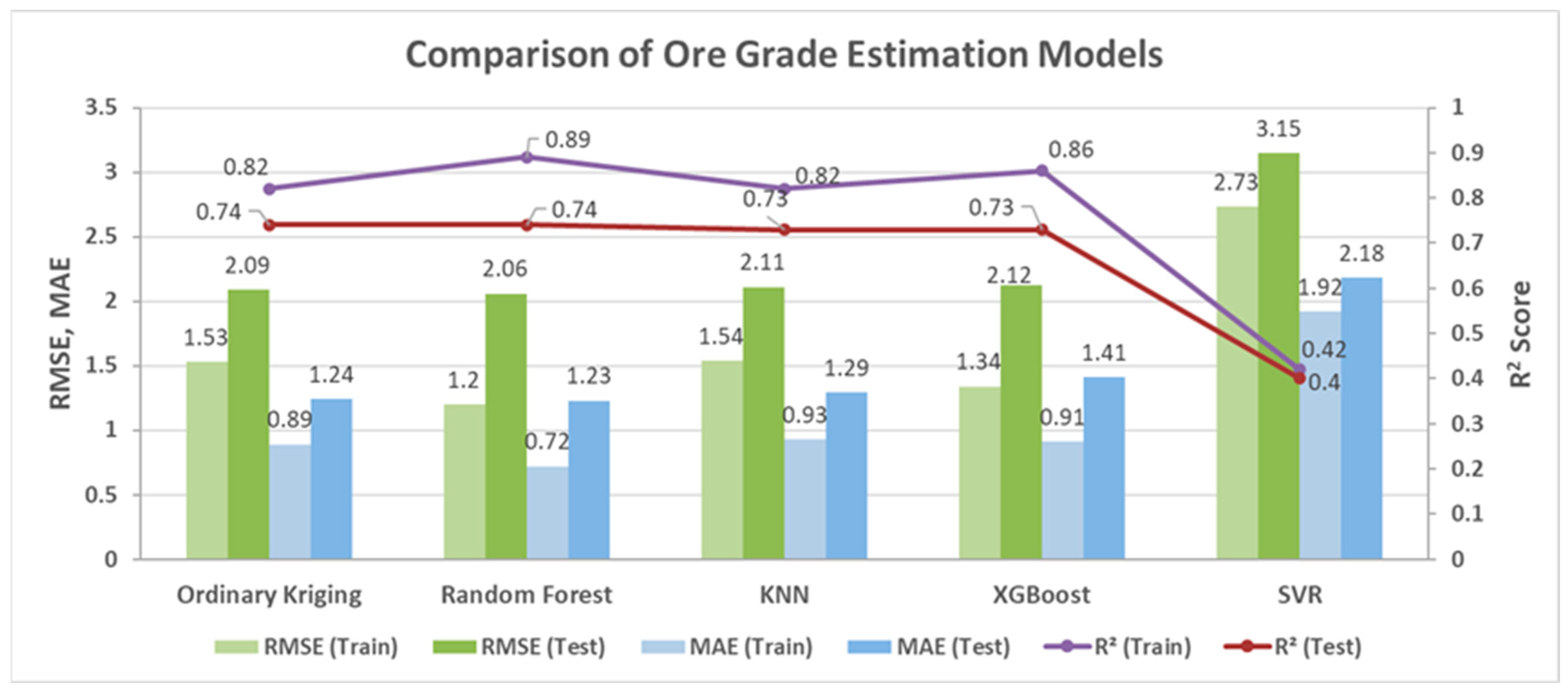
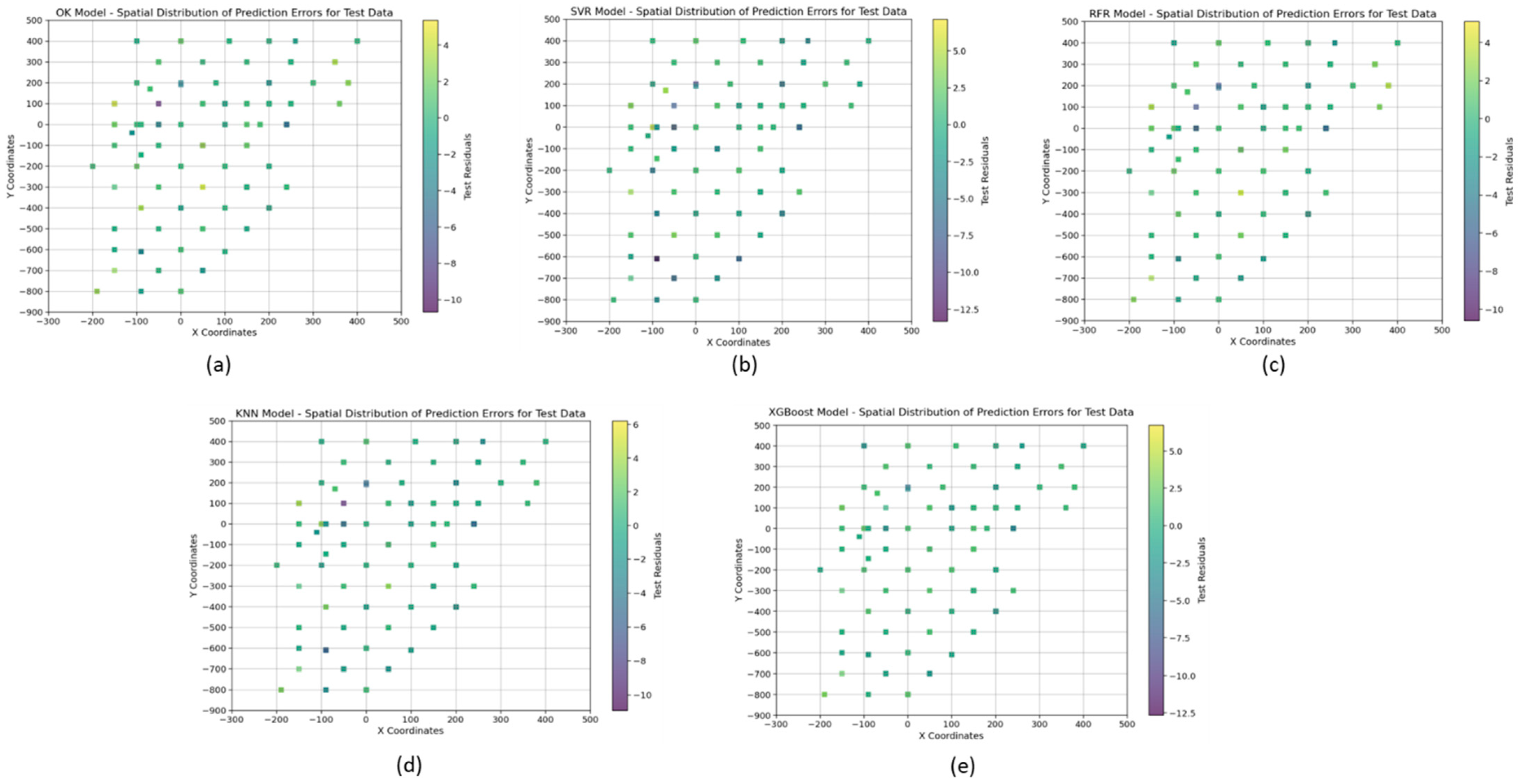
4.6. Comparison of the Ore Grade Estimation Models

A comparison of the performance of four models, SVR, RFR, KNN, and XGBoost, and ordinary kriging in predicting iron ore grades, based on three metrics: R2 Score (in %), RMSE, and MAE are presented in Table 7 and Figure 19. In comparing the performance of the models for estimating the iron ore grade, several key patterns emerge. RFR has the highest R2 among the ML models. It achieves the highest R2 value of 0.74 on the test data, indicating that it explains the highest variance in the data. It also records the lowest error metrics, with a test RMSE of 2.06 and a test MAE of 1.23. It indicates that RFR is effective at capturing the intricacies of the interaction between the iron ore grade and spatial coordinates. KNN (Bagging) and XGBoost also demonstrate strong predictive capabilities, with R2 values of 0.73 and 0.73, respectively, on the test data. Their error metrics are slightly higher than those of random forest, but they remain competitive alternatives offering less overfitting. KNN has the advantage of simplicity and interpretability, while XGBoost offers more flexibility. The three models, RFR, XGBoost, and KNN, although they show slightly larger gaps between their training and testing performances, can be comparable to OK in terms of understanding spatial complexities and prediction accuracy.
Conversely, SVR underperforms significantly, with a test R2 of just 0.40, RMSE of 3.15, and MAE of 2.18, reflecting poor results among ML models. SVR could not capture the underlying patterns in these data and struggles to make accurate predictions, indicating that it is not suitable for this particular iron ore deposit. Kriging, while a valid geostatistical method, achieves a moderate performance with an R2 of 0.74 and a test RMSE of 2.09. Despite its R2 matching with ML models, kriging remains useful in geospatial contexts due to its ability to incorporate additional information of spatial anisotropy directly into the model. However, for this iron ore deposit, the results show that OK has a predictive power close to that of ML models. Overall, RFR, XGBoost, and KNN showed a comparatively similar performance to that of the standard geostatistical-based OK model and could be explored as potential methods for similar iron ore or maybe newer deposits.
The spatial distribution maps of prediction errors depicted in Figure 20 and descriptive statistics in Table 8 provide a detailed evaluation of the ordinary kriging (OK) and machine-learning (ML) models for Fe grade estimation. These maps highlight the spatial error patterns and their variability across the study area. The OK model demonstrated relatively smooth spatial error patterns, reflecting its explicit incorporation of spatial continuity through variogram modelling. This approach allowed OK to effectively capture regional trends. However, its performance declined in areas with sparse data, particularly when the variogram range was exceeded, resulting in underpredictions or overpredictions. The residuals of OK had a mean of –0.25 and a standard deviation (std) of 2.07, with occasional outliers such as a maximum residual of 5.36.
In contrast, the ML models exhibited distinct spatial distribution error behaviour. Random forest regression (RFR) produced stable predictions with a mean residual of –0.23 and a std of 2.12, closely resembling OK’s spatial consistency. The ensemble nature of RFR effectively mitigated localized overfitting, leading to smooth spatial transitions and minimal localized anomalies. Similarly, k-nearest neighbour (KNN) demonstrated effective performance in dense sampling areas, with a mean residual of –0.27 and std of 2.09. While KNN performed well in regions with consistent local patterns, it exhibited slight clustering effects in high-density sampling zones and struggled in heterogeneous areas.
XGBoost displayed notable adaptability to spatial variability, achieving the lowest mean residual (–0.14) among all models, with a comparable std of 2.12. This model effectively captured the spatial complexity but was occasionally sensitive to outliers in certain regions. On the other hand, support vector regression (SVR) struggled to generalize spatial trends, resulting in the largest std (3.13) and abrupt error transitions, particularly in sparse data regions. These inconsistencies highlight SVR’s limitations in capturing the spatial continuity and trends. RFR, KNN, and XGBoost proved to be robust alternatives to OK, delivering accurate and consistent spatial predictions without the need for variogram-based assumptions. However, the higher variability and abrupt transitions in SVR predictions suggest that it may be less suited for applications requiring reliable spatial generalization, such as mine planning.
To evaluate the practical applicability of ore grade estimation models in mining operations, block predictions were generated and compared across models. To generate block predictions, each block is defined with dimensions of 25 m × 25 m × 10 m, and the centroid coordinates (x, y, and z) of this block are given as the input to the prediction model. The pykrige, matplotlib, and seaborn Python libraries are used for the visualization of the result. The plan view of block predictions at z = 800 mRL shown in Figure 21 provides a comparative perspective on the Fe grade estimations generated by ordinary kriging (OK) and machine-learning (ML) models, including support vector regression (SVR), random forest regression (RFR), k-nearest neighbour (KNN), and XGBoost regression.
The visual analysis shows that the OK model, which incorporates spatial continuity through a variogram, produced a smooth spatial grade distribution across blocks capturing regional trends. On the other hand, the ML models, while lacking an explicit spatial continuity modelling, demonstrate their prediction strength by leveraging the spatial input data. The ML block predictions approximate the local and regional trend, although with varying degrees of smoothness in grade distribution. Among the ML models, random forest regression (RFR), XGBoost, and KNN closely align with OK in their block predictions. The descriptive statistics in Table 9 reinforce this observation, with the mean predicted grades for RFR (62.36), KNN (62.42), and XGBoost (62.37) closely aligning with OK (62.38).
Additionally, the standard deviations of these models (2.42, 2.59, and 2.54, respectively) are comparable to OK (2.92), suggesting these models generate stable and geologically coherent results. The lower standard deviation also suggests that the block grades are closely associated with minimal deviations producing a smooth transition of grades. The block predictions of KNN, due to its reliance on neighbourhood-based estimations, shows predictions leaning slightly towards higher grade values. While block predictions of RFR provide smoother spatial distributions due to its ensemble averaging. XGBoost also demonstrates a strong performance, capturing complex spatial patterns with detailed transitions capturing lows and highs, although with a sensitivity to localized anomalies. In contrast, support vector regression (SVR) demonstrates high variability, with a much larger standard deviation (4.22) and an anomalously low minimum predicted grade (44.17). This indicates that SVR’s kernel-based approach struggles to capture the overall distribution effectively and overemphasizes localized variations, which is evident in its block visualizations that show abrupt transitions and inconsistent patterns especially in the north-east and south-west directions.
Although the central tendency and quartiles show a close range for all the models, the histogram plots in Figure 22 reveal a key difference in the distribution of the estimated block grades. SVR clearly produces an inconsistent distribution among all, whereas RFR, KNN, and XGBoost show similar distribution to that of the OK model block predictions. KNN shows a clustering effect with a high concentration around 64% Fe. Overall, the descriptive statistics, block predictions, and histogram visualizations highlight that RFR, KNN, and XGBoost complement the results of OK, offering reliable block predictions with smooth and geologically consistent spatial distributions. In contrast, the variability and sharp transitions in the SVR block predictions limit its applicability for practical mine planning and block-support analyses.

5. Limitation and Future Studies

This study has certain limitations that should be acknowledged. The primary objective of this research was to evaluate the feasibility of using geospatial coordinates (x, y, and z) as inputs for iron ore grade estimation and to determine whether machine-learning models can effectively work with such spatial data. The decision to use only spatial coordinates, and not lithological or geochemical attributes, is based on the intuition that, at new locations, the only readily available data are the spatial coordinates. While this approach aligns with real-world exploration scenarios, it inherently limits the ability of the models to capture the complex geological variability of the deposit. Incorporating additional attributes from the geological database, such as lithology, mineralogy, and geochemical data, could enhance the models’ ability to capture these complexities.
It is important to acknowledge that alternative geostatistical methods, such as log-normal kriging, indicator kriging, or disjunctive kriging, may be better suited for skewed datasets. While the models developed in this study captured patterns comparable to those of ordinary kriging, achieving significantly better estimations would require a much larger and more diverse dataset, incorporating a broader range of geological attributes. Future research could explore the prediction of lithology or geochemical attributes as an intermediate step and, subsequently, use these predictions to estimate Fe grades, potentially unlocking more accurate and robust resource estimation capabilities.
The generalizability of the developed machine-learning models poses another limitation. These models are tailored to the studied iron ore deposit and may not perform equally well in other geological settings without significant retraining and fine-tuning. Additionally, the study explored only a few machine-learning methods (SVR, RFR, KNN, and XGBoost) alongside the geostatistical ordinary kriging technique. Other potentially effective approaches, such as neural networks or hybrid models, were not included.
Future research can address these limitations and build upon the findings of this study. Incorporating additional geological attributes, such as lithology, mineralogy, and geochemical composition, alongside geospatial coordinates, could enhance the robustness and accuracy of ore grade estimation models. Exploring the inclusion of anisotropy information in geostatistical methods may also yield more precise spatial variability predictions.
Expanding the range of machine-learning techniques is another promising direction. Advanced models, such as artificial neural networks (ANNs), could be tested for their ability to capture spatial patterns more effectively. Hybrid approaches that combine geostatistical methods with machine learning could also be explored to leverage the strengths of both techniques. Moreover, future work could focus on improving sampling strategies to include more lower-grade samples, enabling models to generalize better across the full range of grades. Lastly, integrating these models into real-world applications, such as decision-support systems for dynamic resource estimation and mine planning, would validate their practical utility and contribute to the mining industry’s operational efficiency.

6. Conclusions

This research focused on estimating the iron ore grade using exploratory borehole data through the application of machine-learning algorithms, including SVR, RFR, KNN regression, and XGBoost regression. The models used spatial coordinates (x, y, and z) as input features for predicting the iron ore grade. The dataset was split into the train and test sets. The model development was carried out using the train set, while the performance evaluation was performed using the test set. The performance of ML models is then compared to that of the OK model, which produced R2 = 0.74 and RMSE = 2.09. Among all the ML models, RFR performed better, exhibiting a high level of accuracy (R2 = 0.74) with the lowest error metrics (RMSE = 2.06), showing its generalization capability. The model provided reliable predictions across both the training and test datasets. The XGBoost and KNN models also produced similar results with R2 = 0.73 and RMSE = 2.12 for XGBoost and R2 = 0.73 and RMSE = 2.11 for KNN. These three models exhibit their capability of capturing spatial relationships and block predictions similarly to that of OK. In contrast, SVR struggled to deliver accurate predictions, with a low R2 of 0.40 and relatively high RMSE of 3.15. The model’s poor performance, despite extensive hyperparameter tuning, highlights its limitations in handling non-linear relationships inherent in the borehole data. All the models, including OK, showed a relatively higher predictive error when estimating for low-grade values, which may be due to the limited number of data points for these grades in this rich iron ore deposit.
While this study demonstrated the feasibility of using geospatial coordinates for grade estimation, the models’ ability to capture the complex geological variability was constrained by the lack of lithological and geochemical attributes. Future research could address these limitations by incorporating a broader range of geological data and exploring hybrid approaches that combine machine learning and geostatistics. Additionally, advanced methods such as artificial neural networks and more diverse datasets could further improve model accuracy and generalizability. The study reveals the potential application of ML models in ore grade estimation, which is a crucial step in mine planning and design. The results indicate that RFR, XGBoost, and KNN models could be explored in addition to or in combination with geostatistical methods such as OK for resource estimation and mine planning optimization processes in similar iron ore deposits. While ML models could pave the way forward as potential techniques for resource estimation, they require substantial training data and careful hyperparameter tuning to learn spatial relationships effectively.

Author Contributions

M.M.—conceptualization, methodology, investigation, writing—original draft, data preprocessing and analysis, developing of geostatistics, OK, and ML models, Python coding, detailing, and overall analysis; A.G.—writing—original draft, developing of ML models, Python coding, and overall analysis; N.B.T.—writing—original draft, investigation, validation, and writing—review and editing; S.S.R.—conceptualization, resources, methodology, investigation, supervision, validation, and writing—review and editing; G.S.—geostatistics, variogram modelling, writing—original draft, and review and editing; Y.F. and N.O.—visualization, data analysis, validation, investigation, and writing—review and editing; Y.K.—conceptualization, methodology, investigation, and supervision. All authors have read and agreed to the published version of the manuscript.

Funding

This research received no external funding.

Data Availability Statement

The raw data supporting the conclusions of this article will be made available by the authors on request.

Conflicts of Interest

The authors declare no conflicts of interest.

References

  1. Reichl, C.; Schatz, M.; Zsak, G. World mining data. In Minerals Production; International Organizing Committee for the World Mining Congresses: Vienna, Austria, 2014; Volume 32, pp. 1–261. [Google Scholar]
  2. Gupta, D.; Rao, J.V.R.; Ramamurty, V. National geophysical mapping in Geological Survey of India—An impetus to mineral exploration. Innov. Explor. Methods Miner. Oil Gas Groundw. Sustain. Dev. 2022, 455–462. [Google Scholar] [CrossRef]
  3. Ministry of Mines, ‘National Mineral Scenario’, Government of India. Available online: https://mines.gov.in/webportal/nationalmineralscenario (accessed on 1 October 2024).
  4. Abbaszadeh, M.; Ehteram, M.; Ahmed, A.N.; Singh, V.P.; Elshafie, A. The copper grade estimation of porphyry deposits using machine learning algorithms and Henry gas solubility optimization. Earth Sci. Inform. 2021, 14, 2049–2075. [Google Scholar] [CrossRef]
  5. Böhmer, M.; Kucera, M. Prospecting and Exploration of Mineral Deposits; Elsevier: New York, NY, USA, 2013. [Google Scholar]
  6. Isaaks, E.H.; Srivastava, R.M. An Introduction to Applied Geostatistics; Oxford University Press: New York, NY, USA, 1989. [Google Scholar]
  7. Abzalov, M. Introduction to geostatistics. In Modern Approaches in Solid Earth Sciences; Springer: Cham, Switzerland, 2016; Volume 12. [Google Scholar] [CrossRef]
  8. Afeni, T.; Akeju, V.; AE, A. A comparative study of geometric and geostatistical methods for qualitative reserve estimation of limestone deposit. Geosci. Front. 2020, 12, 243–253. [Google Scholar] [CrossRef]
  9. Zimmerman, D.; Pavlik, C.; Ruggles, A.; Armstrong, M.P. An experimental comparison of ordinary and universal kriging and inverse distance weighting. Math. Geol. 1999, 31, 375–390. [Google Scholar] [CrossRef]
  10. Mineralnymi, Z.K. Application of linear geostatistics to evaluation of Polish mineral deposits. Gospod. Surowcami Miner. 2006, 22, 53–65. [Google Scholar]
  11. Matheron, G. Principles of geostatistics. Econ. Geol. 1963, 58, 1246–1266. [Google Scholar] [CrossRef]
  12. Krige, D.G. A Review of the Development of Geostatistics in South Africa. In Advanced Geostatistics in the Mining Industry; Springer: Dordrecht, The Netherlands, 1976; pp. 279–293. [Google Scholar] [CrossRef]
  13. Matheron, G. The Theory of Regionalized Variables and Its Applications; EÌ cole National supeÌ rieure des Mines: Paris, France, 1971. [Google Scholar]
  14. Journel, A.G.; Huijbregts, C.J. Mining Geostatistics; Academic Press: San Diego, CA, USA, 1978. [Google Scholar]
  15. Goovaerts, P. Assessment of Spatial Uncertainty In Geostatistics for Natural Resources Evaluation; Oxford Academic: New York, NY, USA, 1997. [Google Scholar] [CrossRef]
  16. Vann, J.; Guibal, D. Beyond Ordinary Kriging—An overview of non-linear estimation. In Proceedings of the a One Day Symposium: Beyond Ordinary Kriging, Perth, Australia, 30 October 1998; p. 32. [Google Scholar]
  17. Sinclair, A.J.; Blackwell, G.H. Applied Mineral Inventory Estimation; Cambridge University Press: Cambridge, UK, 2002. [Google Scholar] [CrossRef]
  18. Matheron, G. A Simple Substitute for Conditional Expectation: The Disjunctive Kriging. In Advanced Geostatistics in the Mining Industry; Springer: Dordrecht, The Netherlands, 1976; pp. 221–236. [Google Scholar] [CrossRef]
  19. Suro-Pérez, V.; Journel, A.G. Indicator principal component kriging. Math. Geol. 1991, 23, 759–788. [Google Scholar] [CrossRef]
  20. Verly, G.; Sullivan, J. Multigaussian and probability krigings—Application to the Jerritt Canyon deposit. Min. Eng. 1985, 37, 568–874. [Google Scholar]
  21. Bertolini, M.; Mezzogori, D.; Neroni, M.; Zammori, F. Machine Learning for industrial applications: A comprehensive literature review. Expert Syst. Appl. 2021, 175, 114820. [Google Scholar] [CrossRef]
  22. Jung, D.; Choi, Y. Systematic Review of Machine Learning Applications in Mining: Exploration, Exploitation, and Reclamation. Minerals 2021, 11, 148. [Google Scholar] [CrossRef]
  23. Flores, V.; Henriquez, N.; Ortiz, E.; Martinez, R.; Leiva, C. Random forest for generating recommendations for predicting copper recovery by flotation. IEEE Lat. Am. Trans. 2024, 22, 443–450. [Google Scholar] [CrossRef]
  24. Josso, P.; Hall, A.; Williams, C.; Le Bas, T.; Lusty, P.; Murton, B. Application of random-forest machine learning algorithm for mineral predictive mapping of Fe-Mn crusts in the World Ocean. Ore Geology Rev. 2023, 162, 105671. [Google Scholar] [CrossRef]
  25. Bishop, B.A.; Robbins, L.J. Using machine learning to identify indicators of rare earth element enrichment in sedimentary strata with applications for metal prospectivity. J. Geochem. Explor. 2024, 258, 107388. [Google Scholar] [CrossRef]
  26. Gebretsadik, A.; Kumar, R.; Fissha, Y.; Kide, Y.; Okada, N.; Ikeda, H.; Mishra, A.K.; Armaghani, D.J.; Ohtomo, Y.; Kawamura, Y. Enhancing rock fragmentation assessment in mine blasting through machine learning algorithms: A practical approach. Discov. Appl. Sci. 2024, 6, 223. [Google Scholar] [CrossRef]
  27. Samanta, B.; Bandopadhyay, S.; Ganguli, R. Data Segmentation and Genetic Algorithms for Sparse Data Division in Nome Placer Gold Grade Estimation Using Neural Network and Geostatistics. Explor. Min. Geol. 2002, 11, 69–76. [Google Scholar] [CrossRef]
  28. Chatterjee, S.; Bandopadhyay, S.; Machuca, D. Ore grade prediction using a genetic algorithm and clustering Based ensemble neural network model. Math. Geosci. 2010, 42, 309–326. [Google Scholar] [CrossRef]
  29. Goswami, A.D.; Mishra, M.K.; Patra, D. Evaluation of machine learning algorithms for grade estimation using GRNN & SVR. Eng. Res. Express 2022, 4, 035037. [Google Scholar] [CrossRef]
  30. Jafrasteh, B.; Fathianpour, N.; Suárez, A. Comparison of machine learning methods for copper ore grade estimation. Comput. Geosci. 2018, 22, 1371–1388. [Google Scholar] [CrossRef]
  31. Erten, G.E.; Yavuz, M.; Deutsch, C.V. Grade estimation by a machine learning model using coordinate rotations. Appl. Earth Sci. 2021, 130, 57–66. [Google Scholar] [CrossRef]
  32. Erten, G.E.; Erten, O.; Karacan, C.Ö.; Boisvert, J.; Deutsch, C.V. Merging machine learning and geostatistical approaches for spatial modeling of geoenergy resources. Int. J. Coal Geol. 2023, 276, 104328. [Google Scholar] [CrossRef]
  33. Kaplan, U.E.; Topal, E. A New Ore Grade Estimation Using Combine Machine Learning Algorithms. Minerals 2020, 10, 847. [Google Scholar] [CrossRef]
  34. Tsae, N.B.; Adachi, T.; Kawamura, Y. Application of Artificial Neural Network for the Prediction of Copper Ore Grade. Minerals 2023, 13, 658. [Google Scholar] [CrossRef]
  35. Atalay, F. Estimation of Fe Grade at an Ore Deposit Using Extreme Gradient Boosting Trees (XGBoost). Min Met. Explor 2024, 41, 2119–2128. [Google Scholar] [CrossRef]
  36. Bi, Z.; Fu, C.; Zhu, J.; Du, Y. Control Ore Processing Quality Based on Xgboost Machine Learning Algorithm. In Proceedings of the 2023 Asia-Europe Conference on Electronics, Data Processing and Informatics, ACEDPI, Prague, Czech Republic, 17–19 April 2023; pp. 177–180. [Google Scholar] [CrossRef]
  37. Singh, R.K.; Sarkar, B.C.; Ray, D. Geostatistical Modelling of a High-grade Iron Ore Deposit. J. Geol. Soc. India 2021, 97, 1005–1012. [Google Scholar] [CrossRef]
  38. Krishnamurthy, K.V. Reserves and Resources of Iron Ores of India—A Perspective. J. Geol. Soc. India 2022, 98, 647–653. [Google Scholar] [CrossRef]
  39. Devananda, B.; Behera, R. Iron ore localisation and its controlling factors in the eastern limb of Bonai Keonjhar belt, Odisha, India. Int. Res. J. Earth Sci. 2018, 6, 9–15. [Google Scholar]
  40. Indian Bureau of Mines, Nagpur. Gazette Notification for Threshold Value of Minerals, REGD. NO. D. L.-33004/99; Controller of Publications: New Delhi, India, 2018. [Google Scholar]
  41. Cabello-Solorzano, K.; de Araujo, I.O.; Peña, M.; Correia, L.; Tallón-Ballesteros, A.J. The Impact of Data Normalization on the Accuracy of Machine Learning Algorithms: A Comparative Analysis. In Lecture Notes in Networks and Systems; Springer: Cham, Switzerland, 2023; Volume 750, pp. 344–353. [Google Scholar] [CrossRef]
  42. Singh, D.; Singh, B. Investigating the impact of data normalization on classification performance. Appl. Soft Comput. 2020, 97, 105524. [Google Scholar] [CrossRef]
  43. Joseph, V.R. Optimal Ratio for Data Splitting. Stat. Anal. Data Min. 2022, 15, 531–538. [Google Scholar] [CrossRef]
  44. Cortes, C.; Vapnik, V.; Saitta, L. Support-vector networks. Mach. Learn. 1995, 20, 273–297. [Google Scholar] [CrossRef]
  45. Awad, M.; Khanna, R. Support Vector Regression. Effic. Learn. Mach. 2015, 67–80. [Google Scholar] [CrossRef]
  46. Tsirikoglou, P.; Abraham, S.; Contino, F.; Lacor, C.; Ghorbaniasl, G. A hyperparameters selection technique for support vector regression models. Appl. Soft Comput. 2017, 61, 139–148. [Google Scholar] [CrossRef]
  47. Nourali, H.; Osanloo, M. Mining capital cost estimation using Support Vector Regression (SVR). Resour. Policy 2019, 62, 527–540. [Google Scholar] [CrossRef]
  48. Loh, W.Y. Classification and regression trees. WIREs Data Min. Knowl Discov. 2011, 1, 14–23. [Google Scholar] [CrossRef]
  49. Breiman, L.; Friedman, J.H.; Olshen, R.A.; Stone, C.J. Classification and Regression Trees; CRC Press: New York, NY, USA, 2017. [Google Scholar] [CrossRef]
  50. Breiman, L. Random forests. Mach. Learn. 2001, 45, 5–32. [Google Scholar] [CrossRef]
  51. Zhang, H.; Zhou, J.; Armaghani, D.J.; Tahir, M.M.; Pham, B.T.; Van Huynh, V. A combination of feature selection and random forest techniques to solve a problem related to blast-induced ground vibration. Appl. Sci. 2020, 10, 869. [Google Scholar] [CrossRef]
  52. Breiman, L.; Friedman, J.H.; Olshen, R.A.; Stone, C.J. Classification and Regression Trees. Biometrics 1984, 40, 874. [Google Scholar] [CrossRef]
  53. Rai, S.S.; Murthy, V.M.S.R.; Kumar, R.; Maniteja, M.; Singh, A.K. Using machine learning algorithms to predict cast blasting performance in surface mining. Min. Technol. 2022, 131, 191–209. [Google Scholar] [CrossRef]
  54. Dietterich, T.G. Experimental comparison of three methods for constructing ensembles of decision trees: Bagging, boosting, and randomization. Mach. Learn. 2000, 40, 139–157. [Google Scholar] [CrossRef]
  55. Hengl, T.; Nussbaum, M.; Wright, M.N.; Heuvelink, G.B.M.; Gräler, B. Random forest as a generic framework for predictive modeling of spatial and spatio-temporal variables. PeerJ 2018, 6, e5518. [Google Scholar] [CrossRef]
  56. Altman, N.S. An introduction to kernel and nearest-neighbor nonparametric regression. Am. Stat. 1992, 46, 175–185. [Google Scholar] [CrossRef]
  57. Murni; Kosasih, R.; Fahrurozi, A.; Handhika, T.; Sari, I.; Lestari, D.P. Travel Time Estimation for Destination In Bali Using kNN-Regression Method with Tensorflow. IOP Conf. Ser. Mater. Sci. Eng. 2020, 854, 012061. [Google Scholar] [CrossRef]
  58. Öngelen, G.; İnkaya, T. LOF weighted KNN regression ensemble and its application to a die manufacturing company. Sadhana Acad. Proc. Eng. Sci. 2023, 48, 246. [Google Scholar] [CrossRef]
  59. Johannesen, N.J.; Kolhe, M.; Goodwin, M. Relative evaluation of regression tools for urban area electrical energy demand forecasting. J. Clean. Prod. 2019, 218, 555–564. [Google Scholar] [CrossRef]
  60. Chen, T.; Guestrin, C. Xgboost: A scalable tree boosting system. In Proceedings of the 22nd ACM SIGKDD International Conference on Knowledge Discovery and Data Mining, San Francisco, CA, USA, 13–17 August 2016; pp. 785–794. [Google Scholar] [CrossRef]
  61. Friedman, J.H. Greedy function approximation: A gradient boosting machine. Ann. Stat. 2001, 29, 1189–1232. [Google Scholar] [CrossRef]
  62. Bentéjac, C.; Csörgő, A.; Martínez-Muñoz, G. A comparative analysis of gradient boosting algorithms. Artif. Intell. Rev. 2020, 54, 1937–1967. [Google Scholar] [CrossRef]
  63. Daya, S.B.S.; Cheng, Q.; Agterberg, F. Handbook of Mathematical Geosciences: Fifty Years of IAMG; Springer: Cham, Switzerland, 2018; pp. 1–914. [Google Scholar] [CrossRef]
  64. Griffith, D. Spatial Statistics and Geostatistics: Basic Concepts. In Encyclopedia of GIS; Springer: Cham, Switzerland, 2017; pp. 2086–2100. [Google Scholar] [CrossRef]
  65. Dong, W.; Huang, Y.; Lehane, B.; Ma, G. XGBoost algorithm-based prediction of concrete electrical resistivity for structural health monitoring. Autom. Constr. 2020, 114, 103155. [Google Scholar] [CrossRef]
  66. Rossi, M.E.; Deutsch, C.V. Mineral Resource Estimation; Springer: Dordrecht, The Netherlands, 2014; pp. 1–332. [Google Scholar] [CrossRef]
Figure 1. Flowchart showing the process of development of ore grade estimation models.
Minerals 15 00131 g001
Figure 2. Geological map showing iron ore occurrences in Bonai–Keonjhar belt of Odisha, India [38,39].
Minerals 15 00131 g002
Figure 3. Plan view of the boreholes and statistics of boreholes.
Minerals 15 00131 g003
Figure 4. Scatter plot showing the variation of Fe in reference to the features.
Minerals 15 00131 g004
Figure 5. Histogram and box plots showing distribution of Fe %, SiO2 %, Al2O3 %, and spatial coordinates (x, y, z).
Minerals 15 00131 g005aMinerals 15 00131 g005b
Figure 6. Comparison of the distributions of grades of Fe data with train and test sets.
Minerals 15 00131 g006
Figure 7. Comparison of the distributions of grades of Fe data with train and test sets.
Minerals 15 00131 g007
Figure 8. Example of a one-dimensional linear SVR model.
Minerals 15 00131 g008
Figure 9. General structure of a RFR model with details of splitting in decision tree.
Minerals 15 00131 g009
Figure 10. KNN regression for two input variables with k = 5.
Minerals 15 00131 g010
Figure 11. Schematic working flow of XGBoost trees [64].
Minerals 15 00131 g011
Figure 12. Semi-variogram plot showing experimental and theoretical variogram.
Minerals 15 00131 g012
Figure 13. The semi-variogram plot having experimental and theoretical variogram.
Minerals 15 00131 g013
Figure 14. Plots of Fe actual and predicted grades for OK model (Train and Test): (A) model performance; (B) actual vs. predicted; (C) residual error distribution; and (D) residual plot.
Minerals 15 00131 g014
Figure 15. Plots of Fe actual and predicted grades for SVR model (Train and Test): (A) model performance; (B) actual vs. predicted; (C) residual error distribution; and (D) residual plot.
Minerals 15 00131 g015
Figure 16. Plots of Fe actual and predicted grades for RFR model (Train and Test): (A) model performance; (B) actual vs. predicted; (C) residual error distribution; and (D) residual plot.
Minerals 15 00131 g016
Figure 17. Plots of Fe actual and predicted grades for KNN model (Train and Test): (A) model performance; (B) actual vs. predicted; (C) residual error distribution; and (D) residual plot.
Minerals 15 00131 g017
Figure 18. Plots of Fe actual and predicted grades for XGB model (Train and Test): (A) model performance; (B) actual vs. predicted; (C) residual error distribution; and (D) residual plot.
Minerals 15 00131 g018
Figure 19. Comparison of various ore grade estimation models based on performance metrics.
Minerals 15 00131 g019
Figure 20. Spatial distribution of residuals (differences between actual and predicted Fe grades) for (a) ordinary kriging (OK), (b) support vector regression (SVR), (c) random forest regression (RFR), (d) k-nearest neighbour (KNN), and (e) XGBoost.
Minerals 15 00131 g020
Figure 21. Plan view of block prediction results at Z = 800 for (a) OK model, (b) SVR model, (c) RFR model, (d) KNN model, and (e) XGBoost model.
Minerals 15 00131 g021aMinerals 15 00131 g021b
Figure 22. Histogram plots of block predictions of Fe grade values of all models.
Minerals 15 00131 g022
Table 1. Distribution of Fe grade over the intervals.
Hole_idEasting, X (m)Northing, Y (m)Elevation, Z (m)SiO2 (%)Al2O3 (%)Fe (%)
B0150100776.520.700.9253.00
B0150100775.520.080.9353.57
..............
..............
B71–90–145864.51.201.6466.30
B71–90–145850.51.590.9266.33
Table 2. Descriptive stats of the geological database.
Metric Fe (%)SiO2 (%)Al2O3 (%)Easting (X)Northing (Y)Elevation (Z)
Count411241124112411241124112
Mean62.362.712.3087.99–60.65792.08
Std3.673.442.18151.92331. 1943.16
Min50.000.160.02–200–800655.50
25%61.131.001.00–50–300764.50
50%63.591.561.571000.00798.50
75%64.762.872.62200200824
Max68.2025.4025.76400400879
Range18.225.2425.746001200223.5
Skewness–1.423.512.530.13–0.58–0.54
Kurtosis1.514.298.97–0.92–0.57–0.28
Anderson–Darling
Normality test
p-value, normality
p = 0,
non-normal
p = 0,
non-normal
p = 0,
non-normal
p = 0,
non-normal
p = 0,
non-normal
p = 0,
non-normal
Table 3. Descriptive stats of Fe before and after data splitting.
Metric Fe (%)Fe_Train (%)Fe_Test (%)
Count41123495617
Mean62.35862.3762.28
Std3.6653.653.74
Min505050
25%61.1361.2060.80
50%63.5963.6063.50
75%64.7664.7464.86
Max68.268.267.8
Skewness–1.42–1.44–1.34
Kurtosis1.51–1–1.34
Two-sample Z-test p-value 10.860.61
Table 4. Descriptive stats of input and output train–test features after scaling.
Metric Fe_Train (%)Fe_Test (%)X_TrainX_TestY_TrainY_TestZ_TrainZ_Test
Count3495617349561734956173495617
Mean0.00–0.130.000.000.00–0.030.000.07
Std1.001.131.000.991.001.011.001.01
Min–3.47–3.44–1.89–1.89–2.24–2.24–3.14–3.16
25%–0.34–0.58–0.91–0.91–0.73–0.73–0.63–0.56
50%0.330.270.080.080.180.180.140.21
75%0.660.630.740.740.780.750.760.86
Max1.611.612.052.051.391.392.041.95
Skewness–1.44–1.280.130.12–0.58–0.56–0.54–0.56
Table 5. Design details and hyperparameters of the ore grade estimation models.
ModelDesign Features/HyperparametersOptimal Values of Hyperparameters
Ordinary Kriging (OK)-model: ‘spherical’, estimator: matheron,
Range: 508.5, Sill: 13.07, Nugget: 9.08,
n_lags: 16,
anisotropy_angle_x = 0, anisotropy_angle_y = 0, anisotropy_angle_z = 0
Support Vector Regression (SVR)C: [0.01, 0.1, 1, 10, 100, 500],
epsilon: [0.001, 0.01, 0.1, 0.2, 0.5]
kernel: [‘rbf’, ‘poly’]
degree: [2, 3, 4] (only for polynomial),
gamma: [‘scale’, ‘auto’]
C: 500,
epsilon: 0.5,
kernel: ‘rbf’,
gamma: ‘scale’,
Random Forest Regression (RFR)n_estimators: [50, 100, 200]
max_depth: [ 5, 7, 10, 15]
min_samples_split: [2, 3, 4, 5, 6, 7, 8, 9, 10] min_samples_leaf: [2, 3, 4, 5, 6, 7, 8, 9, 10] max_features: [‘sqrt’]
n_estimators: 100,
min_samples_split: 3,
min_samples_leaf’: 2,
max_features: ‘sqrt’,
max_depth: 15
K-Nearest Neighbour (KNN) Regressionn_neighbour: [5, 10, 15, 20],
leaf_size: [30, 40, 50, 60],
n_estimators: [20, 30, 40, 50],
max_samples: [0.7, 0.8, 0.9, 1.0],
metric: [‘euclidean’, ‘manhattan’]
n_neighbour: 5,
leaf_size: 30,
n_estimators: 50,
max_samples: 1.0,
metric: ‘ euclidean’
XGBoost Regressionn_estimators: [50, 100, 200],
learning_rate: [0.01, 0.025, 0.05, 0.075, 0.1], max_depth: [3, 4, 5, 6],
min_child_weight: [2, 5, 10],
gamma: [0.01, 0.025, 0.05, 0.075, 0.1],
booster: [‘gbtree’, ‘dart’]
n_estimators: 100,
learning_rate: 0.1,
max_depth: 6,
min_child_weight: 2,
gamma: 0.075,
booster: ‘dart’
Table 6. Strength and limitation of ML models.
Strengths of ML ModelsLimitations of ML Models
1. Handles Non-Linear Relationships: ML models, like random forest and XGBoost, effectively capture complex, non-linear spatial patterns.1. Lack of Uncertainty Quantification: ML models do not inherently provide measures of prediction uncertainty (e.g., estimation variance for every prediction), which are critical for mining.
2. Flexibility in High-Dimensional Data: ML models can process datasets with numerous variables without strict assumptions.2. Risk of Overfitting: Without careful tuning and cross-validation, ML models may overfit the training data, reducing their generalizability to new data.
3. Robust to Noise: ML models handle noisy and irregular data distributions better than traditional geostatistical methods.3. Potential for Prediction Artifacts: Tree-based models without hyperparameter tunning can produce grid-like artifacts in spatial predictions due to discretized learning processes.
4. No Stationarity Assumptions Required: ML models do not require the stationarity assumption that geostatistical models like OK rely on.4. Limited Geological Context: ML models often rely on the quality and relevance of input features, potentially missing geological interpretations crucial for mining.
5. High Predictive Accuracy: With proper hyperparameter tuning, ML models can outperform traditional methods in terms of predictive metrics.5. Computationally Intensive: Tuning and training sophisticated ML models require significant computational resources and expertise.
6. In practical mining applications, ML models can directly predict grades using spatial data. Therefore, it can minimize the extensive drilling during the exploration stage.6. Site-Specific Models: ML models are often developed for specific mine sites, making it challenging to generalize them to other locations without significant retraining.
Table 7. Comparison of ore grade estimation models based on performance metrics.
ModelR2 (Train)R2 (Test)RMSE (Train)RMSE (Test)MAE (Train)MAE (Test)
OK0.820.741.532.090.891.24
RFR0.890.741.22.060.721.23
KNN0.820.731.542.110.931.29
XGBoost0.860.731.342.120.911.41
SVR0.420.402.733.151.922.18
Table 8. Descriptive statistics of the spatial residual errors of OK and ML models.
MeasurexyzOK Test ResidualsSVR Test ResidualsRFR Test ResidualsXGB Test ResidualsKNN Test Residuals
count617617617617617617617617
mean87.81–69.67794.5551–0.25–0.39–0.23–0.14–0.27
std149.98333.1743.501682.073.132.122.122.09
min–200–800655.5–10.68–13.32–10.74–12.65–10.67
25%–50–300767.5–0.56–1.51–0.63–0.79–0.63
50%1000800.50.000.290.160.160.06
75%200190828.50.611.530.761.050.71
max400400875.55.367.145.026.735.47
Table 9. Descriptive statistics of the block predictions from kriging and ML models.
MeasurexyzOK Block PredSVR Block PredRFR Block PredKNN Block PredXGB Block Pred
count805805805805805804804805
mean60.0–143.780062.3861.5462.3662.4262.37
std139.2346.902.924.222.422.592.54
min–200–82580052.3644.1754.0454.0654.58
25%–50–42580060.2660.8461.0660.5660.75
50%50–12580063.2762.5262.8263.3462.87
75%15015080064.3764.0264.0764.3464.30
max40040080067.1767.6467.9167.0167.11
Disclaimer/Publisher’s Note: The statements, opinions and data contained in all publications are solely those of the individual author(s) and contributor(s) and not of MDPI and/or the editor(s). MDPI and/or the editor(s) disclaim responsibility for any injury to people or property resulting from any ideas, methods, instructions or products referred to in the content.

