Abstract
This study presents a novel lithological analysis method that combines optical thin-section analysis with intelligent algorithms. The method utilizes mineral composition data and two-dimensional rock properties to improve the accuracy and efficiency of lithological identification. By integrating high-resolution optical imaging to precisely capture microscopic rock textures with automated mineral composition analysis systems, this method ensures the rapid and accurate identification of major mineral components without sample damage. Furthermore, advanced image processing and similarity analysis algorithms effectively classify and automatically identify distinct rock layers, enabling a continuous and precise lithological identification process. This approach overcomes the limitations of traditional methods, including subjectivity and inefficiency, and provides robust technical support for geological exploration and mineral resource evaluation. The study shows that this method markedly improves the efficiency of petrological analysis compared to traditional logging techniques. The spatial resolution for mineral composition and lithological identification improved from 12.5 cm to 7 cm per point, maintaining an accuracy of 83%. These results underscore the method’s potential to advance technologies in geoscience and related fields.
1. Introduction
Advances in unconventional oil and gas technologies have spurred growing research interest in inland shale formations. Researchers are investigating the complex lithologies and mineral compositions of these formations [1,2,3]. Enhancing the efficiency and accuracy of engineering geological recognition remains a priority, with machine-learning models supporting uncertainty analysis and optimizing geological models for feature characterization [4,5]. Precise lithology identification is crucial for oil and gas exploration, yet limited lithology labeling constrains machine-learning accuracy [6]. Geng et al. [7] improved formation identification by modeling log maps using unlabeled data and dynamic similarity maps. Logging data serve as a critical tool for lithology interpretation and reservoir evaluation, offering high vertical resolution [8,9,10]. Although conventional logging effectively evaluates clastic and carbonate reservoirs, it faces challenges with shale’s distinct characteristics [11,12]. Petrographic logging models utilizing gamma ray (GR), acoustic logging (AC), and compensated neutron log (CNL) curves facilitate shale evaluation, with lithofacies characterization varying based on mineral composition and sedimentary structures [13,14,15,16].
A hybrid approach combines core drilling data with microscale petrology, scaling logging info and calibrating against imaging, to refine lithofacies division [17]. Reservoir composition logging combines elemental scanning with conventional methods but faces challenges in application and cost. For simple shales, compositional lithofacies division is ideal. Log-based methods incorporating core analysis, X-ray diffraction (XRD), and conventional logging determine mineral content and total organic carbon (TOC). A multi-mineral model based on elastic properties and verified with XRD and logging data provides continuity, though with limited resolution for small-scale details [18].
Elemental scanning logging quickly maps the element distribution in reservoirs, improving precision and detection range compared to conventional methods [19]. Conventional logging curves, such as density and resistivity, are essential for evaluating reservoirs, particularly for identifying key intervals and fractures [20]. However, elemental scanning alone only provides elemental dry weight data. Integrating this with conventional logging, geological data, and X-ray diffraction allows for optimized mineral content models and accurate reservoir assessments [21]. Combining these methods creates a multi-mineral evaluation model for detailed rock classification [22], offering a refined approach to evaluating reservoir properties [23,24]. Distinct sedimentary features in shales provide insights into depositional conditions, revealing diverse features in thin sections [25]. Traditional rock type identification methods include visual inspection for observing color, texture, structure, and mineral crystallinity; thin-section analysis for optical properties and mineral composition [26,27]; and experimental analysis using geophysical and geochemical methods. These methods connect microscopic features to macroscopic data, aiding in reservoir characterization [28,29]. A shale mineral composition model, based on elemental capture spectral logging and thin-section data, supports lithofacies division using techniques like thin-section analysis, XRD, and geochemical testing, focusing on mineral composition and organic carbon [30]. While logging provides continuous physical property measurements, its resolution and model limitations may miss geological details [31]. Coring offers direct lithology observation but is limited by sample quantity, location, and subjective judgment, making comprehensive reservoir characterization challenging [32,33].
The rise of affordable processing technologies like optical thin sectioning and the growing need for mineral mapping have driven research into intelligent mineral identification methods. Continuous large-scale optical data provide centimeter-scale resolution, enhancing the analysis of thin-section data and improving lithology comprehension [34,35]. Understanding rock microstructure and lithology is crucial for enhancing reservoir properties and geological modeling [36]. However, complex lamina morphology complicates lamina type identification, requiring time-consuming manual efforts and geological expertise, especially for large samples. Shales, with their unique stratification, exhibit varying lithology and mineral composition linked to different stratification types [37].
The Advanced Mineral Identification and Characterization System (AMICS) uses electron beam technology, high-resolution backscattered electron (BSE) imaging, and energy-dispersive X-ray spectroscopy (EDS) for precise mineral analysis [38]. It identifies and classifies minerals based on physical and chemical properties, comparing them to a reference library using a Species Identification Protocol [39]. AMICS creates a detailed, statistically representative mineralogical database for researchers [40]. AMICS excels in providing spatially resolved data and modal mineral information, detecting both major and trace minerals effectively. Unlike optical microscopes, which offer image data but lack AMICS’s detail and speed in quantitative analysis, and XRD, which is important but limited in spatial resolution and trace element analysis, AMICS offers accurate, repeatable, and detailed large-scale datasets [41,42,43].
Continuous optical thin sections photo (7 cm by 5 cm) provide centimeter-scale visualization for detailed rock analysis, aiding intuitive lithology understanding and geological modeling. However, complex layered morphologies can complicate identification. This paper introduces a novel intelligent lithology method using statistical analysis and threshold detection to improve shale rock type and mineral content identification. It also presents an image-based annotation algorithm that uses grayscale and Red Green Blue (RGB) histograms for automatic similarity detection, showing high precision and stability in various images, thus enhancing lithology analysis. This study addresses key limitations in traditional lithological analysis, such as low resolution, limited labeling, and labor-intensive methods, by introducing a novel intelligent approach that integrates high-resolution optical imaging, AMICS, and advanced statistical algorithms. This method enhances accuracy and efficiency in identifying shale lithologies, offering scalable solutions for complex geological modeling and reservoir characterization. It combines qualitative and quantitative analyses, enabling precise, automated lamina detection and comprehensive multi-mineral evaluation.
2. Methodology and Research Workflow
This study introduces an innovative lithological classification methodology combining optical thin-section analysis with intelligent algorithms. By leveraging RGB and grayscale four-channel histogram distributions to constrain sub-regional image similarity, the approach achieves precise differentiation of laminae, microstructural details, and mineral textures. Integrating AMICS results with histogram-based mineral proportion estimates ensures consistent and comprehensive minerals identification and lithological classification across scales, the work procedure as shown in Figure 1.
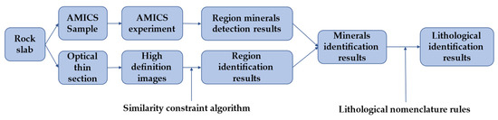
Figure 1.
Flow chart for the work procedure.
2.1. Laminar Type and Characterization
This study employed the Advanced Mineral Identification and Characterization System (AMICS) to obtain detailed mineralogical data by depth, with sample selection guided by optical thin-section classification. Six lamination types were identified based on mineral grain size, primary mineral types, and depositional states observed in optical thin sections. Representative depth samples were selected from residual materials after thin-section preparation for AMICS analysis, as shown in Figure 2.
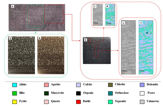
Figure 2.
The optical thin section corresponds to the AMICS experimental selection: (a) Rock slab. (b) Treated samples. (c) BSE image of test area 1. (d) Pseudo-color mineral map of test area 1. (e) BSE image of test area 2. (f) Pseudo-color mineral map of test area 2. (g) Cross-polarized thin section. (h) Plane-polarized thin section.
The AMICS system quantified the primary mineral types for each lamination type. Experimental results were categorized following the conventions in Table 1. Sample size was determined by the thickness of the thinnest lamination to ensure precise lithological identification and classification.

Table 1.
Lithology nomenclature. Where the mud properties include mud-grade terrigenous clastic and clay minerals. (This naming standard is implemented in accordance with thePetroleum Industry Standards SY/T 5368-2016 of the Society of Petroleum Engineers of China) [44].
2.2. Target Recognition Based on Multi-Channel Feature Extraction
Fine-grained layers with a maximum width constrained to a 1900 × 400 pixel area (each pixel representing 0.245 µm2) were selected based on mineral analysis and optical thin-section observations, adhering to lithological naming principles. The minimum recognition accuracy achieved was 465.5 µm in length and 98 µm in width. However, this microscopic precision was insufficient for macroscopic analysis and classification. To address this limitation, an integrated strategy combining AMICS data and continuous optical thin sections was developed.
Input data included plane-polarized and cross-polarized thin-section images obtained under varying polarization techniques to highlight specific physical and chemical properties. Optical thin-section regions matching AMICS coverage were selected for advanced image processing to enhance quality, contrast, and clarity, emphasizing intricate details. Image segmentation techniques delineated distinct regions, enabling precise feature extraction.
A custom algorithm was developed to analyze and quantify complex image data. This algorithm integrates similarity constraints to improve the interpretability of extracted features from six target images (1900 × 400 pixels each). It systematically captures grayscale and RGB information, performing detailed four-dimensional histogram distribution analyses to characterize image features. By applying similarity constraints, the algorithm ensures alignment with meaningful patterns in the data. Each segmented region was compared to target image data to evaluate feature consistency (Figure 3). Grayscale and RGB histograms were normalized for similarity scoring (0 for no match, 1 for a perfect match). These normalized histograms served as benchmarks for comparative analysis, highlighting regions of high similarity and reinforcing the reliability of extracted features.
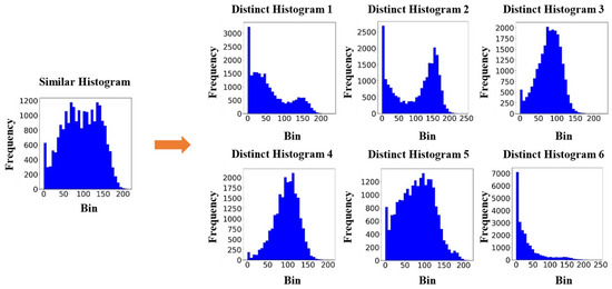
Figure 3.
Histogram matching diagram. The left side shows the histogram distribution of the single region after cutting, and the right side shows the histogram distribution of the six target samples selected.
The similarity metric was calculated using histograms of grayscale and RGB channels. The formula for grayscale similarity is shown in Equation (1), while similarities for the red, green, and blue channels are computed using Equations (2), (3) and (4), respectively. The overall similarity, a weighted sum of these channel-specific similarities, is defined in Equation (5):
Here, and are histograms of the reference and target regions, and represent the image width and height, and are the weight coefficients for the respective channels.
A total of 570 optical thin-section images were analyzed, each subdivided into 1900 sub-regions. As the Figure 4 shows the RGB and grayscale histogram calculations enabled the classification of sub-regions based on similarity to target images. The results were aggregated by tallying the occurrences of each target type across sub-regions, followed by post-processing steps to enhance accuracy and consistency.
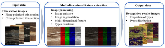
Figure 4.
Algorithm flow chart. Input the original thin section, after image processing get the R, G, B and gray four-dimensional feature extraction than get the recognitions results.
This approach provided detailed characterization of 60 m of continuous six-class mineral layer variations at the thin-section scale. Integration of AMICS experimental data further enriched the analysis by incorporating mineral composition information, enabling precise and continuous mineral distribution mapping. This method effectively bridged the macroscopic–microscopic research gap, overcoming the limitations of traditional logging data.
2.3. Mineral Composition Calculation
An advanced intelligent algorithm was employed to perform multi-layer classification for each optical thin section. By integrating multi-dimensional threshold recognition, a comprehensive sample library, and advanced image recognition techniques, the algorithm accurately identified intricate layer structures. This approach significantly outperformed traditional manual classification methods in both accuracy and efficiency, as shown in Figure 5.
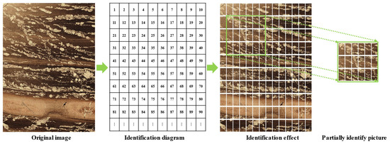
Figure 5.
Example of the regionalization, the images are identified in order to confirm the four-channel characteristics of each region itself.
For detailed regional analysis, the optical thin-section images were divided into sub-regions of 1000 × 400 pixels. A sliding window technique was applied, with a window size of 1000 × 400 pixels and a step size of 400 pixels, to systematically scan the entire image. Each sub-region underwent similarity comparisons with six predefined target types, ensuring comprehensive and precise classification across the thin section. Following the classification process, the AMICS was utilized to analyze the mineral composition of each target type. AMICS provided precise quantification of the major, minor, and trace minerals, delivering high-resolution data crucial for calculating mineral proportions.
Matrix operations were then conducted to compute the dot product of the classification results and mineral composition data from AMICS. This integration enabled accurate and efficient calculations of overall mineral proportions in each thin section, ensuring systematic consistency and comprehensiveness. To standardize the data for cross-sample comparisons, normalization procedures were applied to scale mineral proportions within a predefined range (e.g., 0 to 1). This step minimized variations due to differences in mineral types and compositions, enhancing the comparability, scientific rigor, and reliability of the results.
3. Geological Context and Study Area
In this study, a borehole in a hydrocarbon-rich depression within the northwestern margin of the Junggar Basin, an important intracontinental sedimentary basin in northwestern China, was selected as the primary research object. The Junggar Basin has a complex geological history characterized by multistage tectonic movements and sedimentation processes. It hosts various depositional environments, including lacustrine, deltaic, and fluvial systems, resulting in sedimentary rock assemblages dominated by mudstone, sandstone, and carbonate rocks. The Permian strata in this region predominantly consist of fine-grained sedimentary rocks, including light black mudstone, argillaceous dolomite, and dolomite siltstone, characterized by frequent vertical interbedded structures. The study area exhibits complex lithofacies variations, posing challenges to geological analysis while underscoring the critical importance of laminar characterization. Laminar characterization provides critical insights into stratal distribution patterns, diagenetic evolution processes, and their relationship with reservoir performance, offering a robust geological foundation for accurately characterizing reservoir structures and predicting favorable zones [18,45]. Thus, conducting fine-scale characterization in this area of complex lithofacies changes is invaluable for formulating effective oil and gas exploration and development strategies. Following coring, the longitudinal central portion of the full-size core was sectioned to produce large rock slabs, which were subsequently used for optical thin-section preparation [46]. Following core retrieval, the longitudinal central portion of the full-size core was sectioned to produce large rock slabs for optical thin-section preparation. A total of 570 large optical thin sections were prepared from rock slab samples within a depth interval of 60 m, as illustrated in Figure 6.
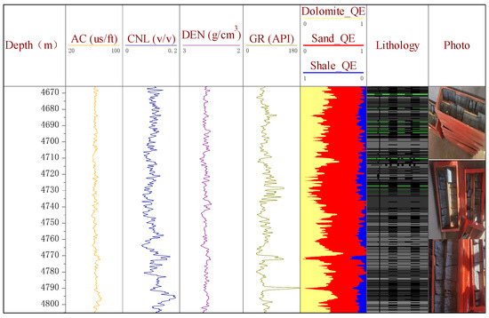
Figure 6.
Comparison of conventional well-logging data (acoustic logging, density logging, compensating neutron logging, and gamma logging), mineral distribution curves, lithology distribution, and large rock plate images.
4. Laboratory Experiment
4.1. Light Microscope Observation
To enhance the resolution of formation changes, continuous optical thin sections were prepared from each rock slab, sampled systematically based on identified characteristics. Figure 7 illustrates three consecutive samples taken from the left rock slab. The large-area full-field imaging system, comprising a multifunctional microscope, automated image acquisition platform, and high-definition (HD) image processing system, facilitated this process.
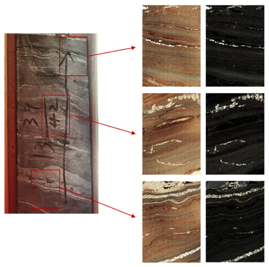
Figure 7.
Optical thin sections were prepared from large rock slabs, with samples selected based on identified features. The figure illustrates three consecutive thin sections taken from the left rock slab.
Standard thin sections measure approximately 2 cm × 5 cm, while the large thin sections used in this study are around 5 cm × 7 cm and 0.03 mm thick, providing detailed mineralogical information (Figure 8). High-resolution images were captured across multiple fields of view using an automated x-y translation platform and stitched into panoramic HD images with five million pixels. Precision-cut and polished slices, impregnated and sealed to enhance stability and transparency, were prepared to ensure micron-scale thickness and optimal microscopy results.
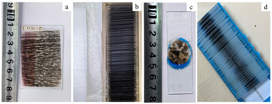
Figure 8.
The different of large thin section and normal thin section. (a) Large thin section. (b) Large thin-section box. (c) Normal thin section. (d) Normal thin-section box.
Observations of optical thin sections under the microscope reveal distinct morphological and color characteristics of various minerals critical for their identification [47]. For instance, quartz appears as granular, colorless to light gray structures, while feldspar exhibits platy forms with pale hues. Amphibole minerals display long prismatic morphologies with characteristic green or brown tones. The extinction characteristics under polarized light provide additional insights into mineral crystallography and optical properties. The selected samples from this well section exhibit unique sedimentary states and mineral compositions, as illustrated in Figure 9. In Figure 9, subfigures (a) and (b) exhibit the presence of coarse-grained intrusions and unstable depositional conditions. Subfigures (c) and (d) depict regular and stable sedimentary patterns. Subfigures (e) and (f) illustrate wavy depositional features within argillaceous laminae, while subfigures (g) and (h) display alternating wavy deposition of argillaceous and silt-sized mineral phases. Integrating these observations and criteria allows for a preliminary identification of mineral types. Additionally, a detailed analysis of mineral grain size and depositional state facilitates a more accurate differentiation of distinct lamination types [48].
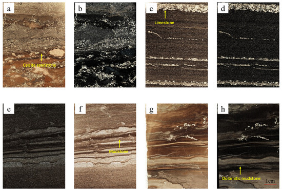
Figure 9.
Four groups of plane-polarized thin section and cross-polarized thin section. (a) 4730.78–4730.85 m plane-polarized thin section. (b) 4730.78–4730.85 m cross-polarized thin section. (c) 4739.65–4739.72 m plane-polarized thin section. (d) 4739.65–4739.72 m cross-polarized thin section. (e) 4796.23–4795.30 m plane-polarized thin section. (f) 4796.23–4795.30 m cross-polarized thin section. (g) 4716.74–4716.82 m plane-polarized thin section. (h) 4716.74–4716.82 m cross-polarized thin section.
Based on the characteristics of the optical thin section, six samples at the same depth were selected for the AMICS experiment to obtain stratified mineral composition information to improve the understanding of the continuous dominant mineral composition and lithology of the horizon.
4.2. AMICS
The Advanced Mineral Identification and Characterization System (AMICS) is an automated tool for efficient and precise mineral identification, combining Scanning Electron Microscopy–Backscattered Electron (SEM-BSE) imaging with energy-dispersive spectroscopy (EDS) analysis. BSE images provide atomic number contrast, while EDS determines elemental composition, enabling comprehensive classification and characterization of mineralogical and textural properties. This approach automates the generation of mineral distribution maps and quantitative composition data, reducing the subjectivity and inefficiency of manual methods.
For large fields of view, AMICS employs automated image stitching to maintain high resolution. Mineral identification is performed point by point by comparing energy spectrum curves to reference data in the mineral library, generating false-color maps where distinct colors represent different minerals as in Figure 10 [49]. While AMICS provides high accuracy and efficiency, limitations include an inability to distinguish mineral isomers and a resolution constrained by characteristic X-rays, typically up to 0.8 μm [50]. Additionally, its sensitivity to low-density minerals, such as organic matter, is limited. To address these challenges, mineral maps are often cross-referenced with higher-resolution BSE images to extract more detailed geological information [51].
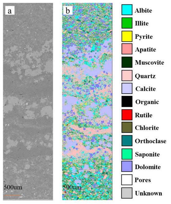
Figure 10.
Mineral analysis results of the sample in this experiment. The test area is 1501 µm × 6397 µm, and the minimum segment is 0.245 µm. In the resulting image, the identified output image size is 6144 × 26164 pixels. The total test time is about 3 h. (a) BSE image of test area. (b) Pseudo-color mineral map and color scale of mineral.
5. Results
5.1. Mineral Distribution
According to the selection results in Figure 11, we select the thickness of the finest grain layer and the appropriate width to set the target sample size and then correspond to the position of the optical slice according to its smallest region, as shown in Figure 12. For each small target region, there are four types of pictures, respectively, plane-polarized image; cross-polarized image; BSE image; and pseudo-color mineral map image.
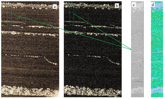
Figure 11.
The optical thin section corresponds to the AMICS experimental selection: (a) plane-polarized thin section; (b) cross-polarized thin section; (c) BSE image of test area; (d) pseudo-color mineral map of test area.
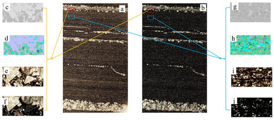
Figure 12.
The optical thin section corresponds to the AMICS experimental selection (a) plane-polarized thin section; (b) cross-polarized thin section; (c) target 1 BSE image; (d) target 1 pseudo-color mineral map of test area; (e) target 1 plane-polarized thin section; (f) target 1 cross-polarized thin section image; (g) target 1 BSE image; (h) target 1 pseudo-color mineral map of test area; (i) target 1 plane-polarized thin section; (j) target 1 cross-polarized thin section image.
A detailed examination of mineral proportion data across distinct laminae reveals critical geological characteristics, shedding light on significant variations in mineral composition and their potential genetic origins. Leveraging optical thin-section analyses and quantitative data from the AMICS experiments, the laminae within this interval were classified into six distinct types. While the AMICS experiment provides mineral proportion data for the entire experimental area, this study refines the analysis by employing color proportions extracted from pseudo-colored mineral maps to estimate the mineral composition of the target regions with enhanced precision.
In geology, rocks are classified based on compositional characteristics, including mineral composition and relative proportions. This classification process emphasizes a comprehensive analysis of the overall mineral composition of the rock, rather than focusing solely on individual mineral grains. In this study, the quantities of quartz, dolomite, calcite, and clay minerals were quantified, with supplementary observations from optical thin sections, to ensure accurate rock classification and nomenclature. The mineral proportion results are summarized in Table 2, with lithology determined through the integration of mineral proportion data and optical thin-section observations.
Table 2.
Laminar types and mineral proportion.
Furthermore, the histogram distribution characteristics of four channels corresponding to the six identified lamina types demonstrate distinct patterns, facilitating their differentiation, as shown in Figure 13. The six lamina types are classified as dolomitic mudstone, dolomite-bearing mudstone, calcite sandstone, argillaceous limestone, mudstone, and calcite mudstone. The inspection results of the corresponding images are illustrated in Figure 14.
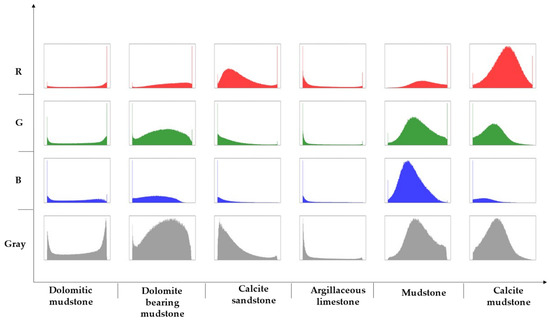
Figure 13.
Four channel histogram distribution characteristics of these six layers. The ordinate is the four channels of image color, and the abscissa is the six lithological names.
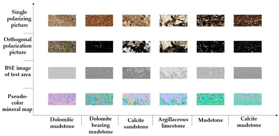
Figure 14.
Laminar types images. The ordinate is the four experimental results, and the abscissa is the six lithological names.
Quartz enrichment in dolomitic mudstone and argillaceous limestone indicates stable depositional environments with minimal post-depositional alteration. The decline in quartz content observed in the upper laminae may reflect environmental transitions or the influence of diagenetic processes. Variations in albite proportions suggest fluctuating geological conditions, with elevated levels in calcite sandstone potentially associated with alkaline environments or specific diagenetic mechanisms. The interplay between quartz and albite proportions underscores their competitive growth dynamics. Meanwhile, the presence of chlorite, muscovite, orthoclase, illite, and pyrite is indicative of rock alteration processes, fluid chemistry, and redox conditions, providing critical insights into the depositional and diagenetic history of these rocks. Pore proportion variations highlight differences in rock density, which are essential for assessing reservoir potential. The limited presence of rutile and apatite further suggests that these laminae are not enriched in accessory minerals, offering additional constraints on the mineralogical and geochemical characteristics of the studied intervals.
In summary, the varying proportions and distribution patterns of these minerals provide valuable insights into their origins, depositional environments, and diagenetic histories. Analyzing these data carefully can enhance our models of lamina formation and evolution, advancing research in geology, petrology, and related fields.
5.2. Hierarchical Recognition Result
Through a comprehensive analysis of stratigraphic information derived from continuous optical thin sections, the integration of recognition results from plane-polarized and cross-polarized images facilitates precise stratification of the samples. Plane-polarized images excel in delineating the macrostructural framework of the formation by capturing distinct textural and compositional features. In contrast, cross-polarized images enhance the detection of subtle microstructural variations, leveraging their sensitivity to fine material properties.
The combined application of these imaging techniques offers a robust representation of subtle stratigraphic changes, providing a detailed and accurate depiction of hierarchical characteristics. This integrative approach not only improves the clarity of stratified structures but also enables in-depth analysis of layer transition relationships, material composition variations, and potential geological phenomena, such as deformation. Representative recognition results are illustrated in Figure 15.
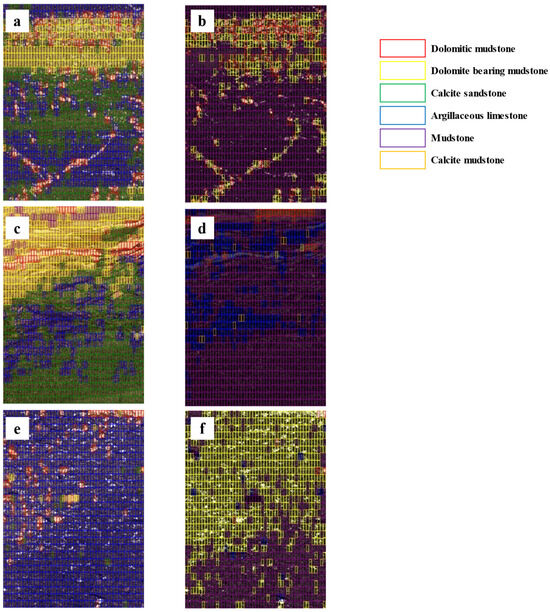
Figure 15.
Hierarchical recognition results. Colored boxes represent different lithology results: (a,c,e) show single-polarized picture recognition results, while (b,d,f) display orthogonal-polarized picture recognition results.
5.3. Identification Result
Through meticulous identification of continuous optical thin sections and comprehensive analysis of mineral composition percentages, the detailed lithological characteristics of various target well intervals have been established.
In Well Interval 9, shown in Figure 16, a total of 117 thin sections were analyzed, revealing a diverse lithological composition. Dolomitic mudstone was identified as the dominant lithology, encompassing 37 sections, indicative of its extensive distribution within this interval. Calcite sandstone, comprising 34 sections, was the second most prevalent lithology, highlighting its significant presence. Argillaceous limestone, represented by 33 sections, ranked third, further emphasizing the stratigraphic diversity of this unit.
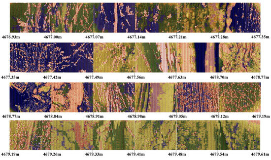
Figure 16.
Part of the recognition partition results in Well Interval 9 of continuous 1.68 m by single-polarized picture.
In Well Interval 12, shown in Figure 17, the analysis of 84 thin sections revealed that argillaceous limestone emerged as the primary lithology, occupying 35 sections, highlighting its significant presence at this depth. Dolomitic mudstone followed suit, with 24 sections, ranking second. Calcite sandstone, with 18 sections, completed the lithological profile as a supporting component.
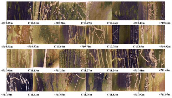
Figure 17.
Part of the recognition partition results in Well Interval 12 of continuous 1.68 m by single-polarized picture.
Well Interval 15, shown in Figure 18, encompassed 135 thin sections, yielding a more intricate lithological picture. Dolomitic mudstone dominated with 64 sections, while argillaceous limestone, with 38 sections, played a substantial role as a secondary lithology. Calcite sandstone, represented by 28 sections, contributed to the overall lithological composition of this interval.
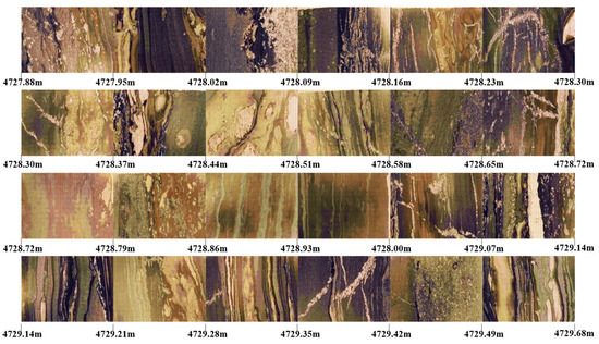
Figure 18.
Part of the recognition partition results in Well Interval 15 of continuous 1.68 m single-polarized picture.
In Well Interval 19, shown in Figure 19, the analysis indicated that over half (38 sections) of the 68 thin sections were identified as dolomitic mudstone, emphasizing its high concentration and significance within this layer.
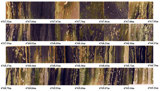
Figure 19.
Part of the recognition partition results in Well Interval 18 of continuous 1.68 m single-polarized picture.
Lastly, for Well Interval 21, shown in Figure 20, a comprehensive analysis of 176 thin sections revealed a more complex lithological assemblage. Dolomitic mudstone stood out as the core lithology, accounting for 93 sections. Calcite mudstone, with 44 sections, served as an essential addition, enriching the dimension of lithological analysis. This outcome not only reflects the intricate variability of subsurface lithology but also provides valuable data support for our in-depth understanding of underground geological structures.
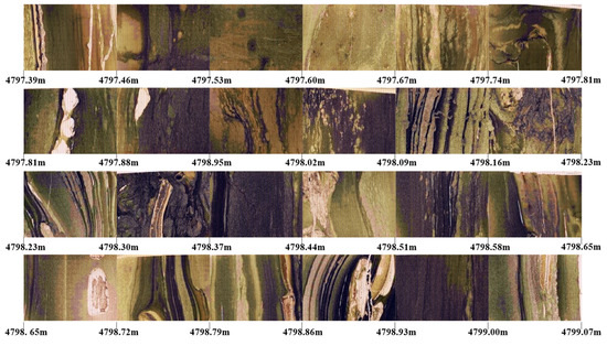
Figure 20.
Part of the recognition partition results in Well Interval 21 of continuous 1.68 m single-polarized picture.
6. Discussion
6.1. Comparative Analysis of Mineralogical Composition
This study integrates logging data with AMICS technology and multi-channel image analysis of single-polarized thin sections to characterize the mineral composition and lithology of shale reservoirs in the Junggar Basin. The primary mineral constituents analyzed include quartz, feldspar, carbonate minerals, and clay minerals, with quartz being the dominant phase. Logging data reveal quartz content ranging from 0% to 73.46% (average: 46.79%) and feldspar content from 0% to 62.27% (average: 21.72%). Carbonate minerals, particularly calcite (average: 14.76%) and dolomite (average: 7.92%), exhibit varying abundances, while clay minerals (average: 7.3%) and pyrite (average: 1.5%) are present in lower proportions, with the latter potentially influencing reservoir characteristics. The mineral components result by logging date are shown in Figure 21.
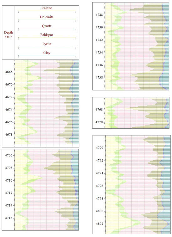
Figure 21.
Mineral composition proportion results of log data of five well sections.
Further research reveals that logging data from different depth intervals adequately reflects the heterogeneity of mineral composition. Within the depth range from the ninth to the twenty-first well interval, calcite and dolomite contents fluctuate, with calcite being slightly more abundant overall. Minerals such as quartz and potassium feldspar exhibit similar trends. These observations indicate the complex geological conditions influencing mineral distribution. Despite its low content, pyrite may significantly impact reservoir properties and oil and gas generation [52]. The content and type of clay minerals, as critical components of shale reservoirs, substantially affect reservoir permeability and storage capacity [53]. Variations in logging response values with depth response values of some minerals exhibit fluctuating or increasing trends which are potentially related to changes in underground temperature, pressure, and other factors. These trends underscore the heterogeneity in mineral content and distribution.
Depth interval analyses (Figure 22) further reveal distinct mineralogical trends. Fluctuations in calcite and dolomite contents reflect heterogeneity influenced by geological conditions. Refined mineral identification results based on the AMICS experiment and optical thin-section similarity algorithm, with a spatial resolution of 7 cm, significantly enhanced mineral distribution analysis and lithology classification. Quartz dominates with an average proportion of 31.05%, while feldspars, including albite (16.10%) and orthoclase (4.92%), display stable distributions. Calcite (mean: 27.48%) and dolomite (mean: 9.25%) exhibit notable heterogeneity, with calcite ranging from 0.15% to 59.01%.
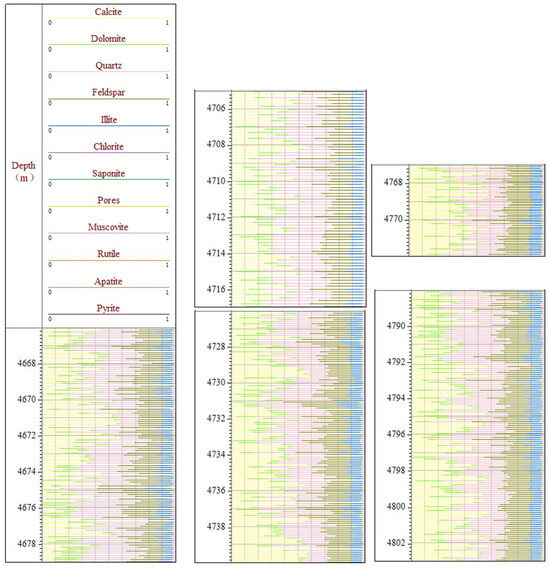
Figure 22.
Identification results of mineral composition proportion based on similarity constraint optical thin sections for five well sections.
Clay minerals, such as chlorite, illite, and saponite (mean: 7.5%), contribute to the geochemical profile. Minor minerals, including muscovite, rutile, apatite, and pyrite, provide insights into reservoir genesis and diagenesis. Although minimal (average pore content: 0.58%), pores are critical for reservoir evaluation.
The integration of logging data, AMICS technology, and advanced imaging techniques reveals significant mineralogical complexity and heterogeneity within the shale reservoirs of the Junggar Basin. The mineral composition is predominantly characterized by felsic and carbonate minerals, with quartz as the most abundant constituent. Variations in mineral proportions reflect the influence of diverse geological conditions, emphasizing the complexity of mineral associations in the region.
Quartz, feldspar, and calcite dominate the mineral composition across both logging data and thin-section analyses, underscoring their central role in the studied samples. Collectively, these three minerals are consistently present in 331 out of 570 samples (58%), reflecting their representativeness in the mineral assemblages. In cases where two minerals coexist, quartz is invariably present, highlighting its pivotal role within the mineralogical framework, particularly in similar sedimentary environments [54]. Quartz’s dominance in similar sedimentary environments. Clay minerals, including chlorite, illite, and saponite, contribute to the geochemical profile, providing critical insights into diagenetic processes.
This study demonstrates the robust capabilities of integrating logging data with AMICS technology for refining mineralogical analyses and lithological classification. By linking results to geological interpretations and situating findings within a broader scientific context, this research contributes to advancing shale reservoir characterization and hydrocarbon exploration.
Despite these insights, the methodology is constrained by the resolution-scale trade-off, with detailed analyses restricted to selected target regions (1900 × 400 pixels). This limitation may reduce the ability to analyze broader geological features. Furthermore, the assumption that target regions are representative of the entire sample introduces potential biases. Addressing these challenges requires calibration of region selection and complementary multi-scale analyses. Future research should focus on integrating high-resolution imaging with advanced computational techniques to enhance scalability while maintaining precision. Additionally, combining AMICS technology with isotopic and geochemical analyses could further elucidate the genesis and evolution of mineral assemblages in shale reservoirs.
6.2. Enhanced Lithological Classification Through Thin-Section and Well-Logging Integration
Accurate rock property identification is essential for understanding subsurface structures, tectonic evolution, and hydrocarbon exploration. This study introduces a refined lithological classification method based on precise nomenclature rules, achieving a resolution of 98 microns—significantly higher than the 12.5 cm resolution of conventional well-logging data.
Among 570 analyzed samples, 17% showed discrepancies due to geological complexities, while 65% exhibited strong consistency, including 18% with complete agreement. Thin-section analyses excel at capturing microstructural details such as mineral proportions, pore networks, and lamina textures. This contrasts with the broader physical rock property insights and stratigraphic trends provided by well-logging. A lithological correlation diagram (Figure 23) highlights the superior stratigraphic segmentation achieved through this methodology, reinforcing its applicability in detailed lithological characterization.
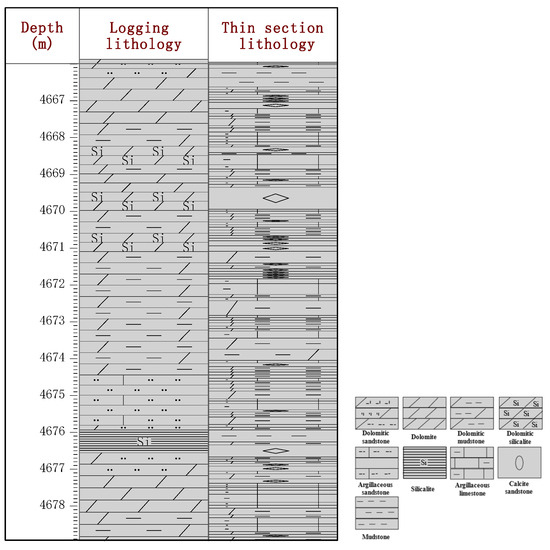
Figure 23.
A part of the lithology correlation diagram (4676.93–4679.33 m). Lithology map of logging data and lithology map identified by optical thin section; right is the lithology legend.
The significance of microstructural analyses in lithology has been well-documented [55]. The method’s ability to capture heterogeneity at the microscopic scale offers valuable insights into depositional processes and diagenetic alterations. However, the resolution trade-offs between well-logging and thin-section data require a multi-faceted approach for holistic geological interpretations. Despite its strengths, the methodology faces notable challenges. The restriction to target regions (1900 × 400 pixels) limits macroscopic geological feature analysis, posing challenges for large-scale interpretations. Additionally, assumptions about the representativeness of target regions may introduce biases, particularly in heterogeneous samples. These limitations necessitate careful calibration of region selection and integration of multi-scale analyses.
In summary, integrating thin-section analyses with well-logging data demonstrates significant potential for advancing lithological characterization. While thin sections refine classifications at the micro-scale, well-logging provides macro-scale perspectives on physical rock properties and stratigraphic continuity. Addressing resolution-scale trade-offs and improving computational efficiency will further strengthen this synergy.
This study underscores the importance of incorporating diverse techniques for lithological characterization. By addressing macro- and micro-level variations and fostering innovations in methodology, this approach lays the groundwork for more precise resource exploration and geological research. The development of fusion technologies for integrating complementary methods will be pivotal in advancing the efficiency and accuracy of rock property identification.
6.3. Discussion on Methods
The application of RGB and grayscale four-channel histogram distribution results from six target images to constrain sub-regional image similarity in large-scale optical thin-section images presents both advantages and limitations in predicting overall image categories. Optical thin sections encompass a wide range of mineralogical and stratigraphic information, making this approach particularly valuable for identifying and analyzing color features.
This approach has demonstrated robustness and practical utility in tasks such as stratigraphic division and rock classification. This method effectively leverages multi-channel histogram to differentiate mineral types and stratigraphic features within optical thin sections. The sub-regional similarity constraint allows for precise analysis of local variations within the thin section, reducing the impact of outliers on the overall classification results. Additionally, by combining AMICS experimental results from sample regions identified via similarity algorithms with mineral proportion results derived from the histogram-based similarity constraints, this method yields refined mineral proportion estimates. These estimates, when applied to lithological naming principles, provide consistent and reliable lithology classification results, further enhancing its practical value.
Despite its strengths, the histogram-based similarity method faces inherent limitations. Variability in sample preparation, illumination conditions, and color space changes can significantly influence histogram results, introducing potential errors. Additionally, the intricate boundaries and transitional zones of minerals and stratigraphic layers pose challenges for accurate sub-regional segmentation, particularly in samples with complex mineral compositions or significant microstructural diversity. The reliance on histogram features alone may not fully capture the complexity of optical thin sections.
In conclusion, utilizing RGB and grayscale four-channel histogram distributions for optical thin-section image classification provides an efficient and reliable tool for mineralogical and stratigraphic identification. Enhancing its accuracy and expanding its applicability will deepen insights into mineralogical and stratigraphic features across diverse geological contexts, contributing to a more comprehensive understanding of Earth’s subsurface complexities.
7. Conclusions
- This study is grounded in the analysis of optical thin-section samples, ensuring that the primary lithological characteristics of the target area are accurately captured. By integrating RGB and grayscale four-channel histograms with AMICS experimental results, the intelligent model employs statistical algorithms and threshold constraints to identify specific features. This approach enables the precise identification of layer types and significantly enhances the efficiency of mineral composition and lithology classification, providing a reliable multiscale tool for analyzing mineralogical and structural characteristics.
- The proposed method demonstrates significant improvements in efficiency and accuracy, addressing challenges in lamina identification and mineral composition analysis across diverse geological contexts. It enhances classification precision by incorporating advanced segmentation algorithms, leading to measurable gains in lithological identification.
- Future optimizations will aim to refine segmentation techniques and integrate additional features, such as mineral textures and microstructure patterns, to better address the complexities of optical thin-section analysis. These advancements are anticipated to further enhance the method’s precision and practicality. Additionally, expanding the dataset to encompass diverse regions and lithological types will improve the technique’s generalizability and robustness, ensuring broader applicability in various geological contexts.
- The method’s adaptability enables its application to diverse geological studies, including stratigraphic correlation, reservoir characterization, and mineral exploration. By tailoring the histogram-based analysis to region-specific lithologies and depositional environments, the approach ensures versatility and effectiveness under various imaging and geological conditions.
Author Contributions
Conceptualization, Z.S. and Y.J.; methodology, Z.S., Y.J. and H.P.; validation, Z.S., Y.L. and H.P.; formal analysis, Z.S. and Y.L.; investigation, Z.S.; resources, X.G.; data curation, X.G.; writing—original draft preparation, Z.S.; writing—review and editing, Y.L., H.P. and X.G.; visualization, Z.S. and Y.L.; supervision, Y.J.; project administration, Y.J.; funding acquisition, Y.J. and H.P. All authors have read and agreed to the published version of the manuscript.
Funding
This research was funded by the National Natural Science Foundation of China, grant number 52104013; the National Natural Science Foundation of China, grant number 52334001; and the Science Foundation of China University of Petroleum, grant number 2462024YJRC021.
Data Availability Statement
The datasets used and/or analyzed during the current study are available from the corresponding author on reasonable request.
Conflicts of Interest
The authors declare no conflicts of interest.
References
- Fang, X.; Yang, Z.; Yan, W.; Guo, X.; Wu, Y.; Liu, J. Classification evaluation criteria and exploration potential of tight oil resources in key basins of China. J. Nat. Gas Geosci. 2019, 4, 309–319. [Google Scholar] [CrossRef]
- Yirenkyi, S.; Boateng, C.D.; Ahene, E.; Danuor, S.K. Automatic lithology identification in meteorite impact craters using machine learning algorithms. Sci. Rep. 2024, 14, 14360. [Google Scholar] [CrossRef]
- Han, Z.; Wang, G.; Wu, H.; Feng, Z.; Tian, H.; Xie, Y.; Wu, H. Lithofacies Characteristics of Gulong Shale and Its Influence on Reservoir Physical Properties. Energies 2024, 17, 779. [Google Scholar] [CrossRef]
- Li, M.; Chen, C.; Liang, H.; Han, S.; Ren, Q.; Li, H. Refined implicit characterization of engineering geology with uncertainties: A divide-and-conquer tactic-based approach. Bull. Eng. Geol. Environ. 2024, 83, 282. [Google Scholar] [CrossRef]
- Liu, F.; Lin, P.; Xu, Z.; Shao, R.; Han, T. Extraction and imaging of indicator elements for non-destructive, in-situ, fast identification of adverse geology in tunnels. Int. J. Min. Sci. Technol. 2023, 33, 1437–1449. [Google Scholar] [CrossRef]
- Zhang, L.; Xu, S.; Jin, K.; Zhang, X.; Liu, Y.; Chen, C.; Liu, R.; Li, M.; Li, J. Study on the Influencing Factors of Oil Bearing and Mobility of Shale Reservoirs in the Fourth Member of the Shahejie Formation in the Liaohe Western Depression. Energies 2024, 17, 3931. [Google Scholar] [CrossRef]
- Geng, Z.; Liu, J.; Li, S.; Yang, C.; Zhang, J.; Zhou, K.; Tang, J. Channel attention-based static-dynamic graph convolutional network for lithology identification with scarce labels. Geoenergy Sci. Eng. 2023, 223, 211526. [Google Scholar] [CrossRef]
- Joshi, D.; Patidar, A.K.; Mishra, A.; Mishra, A.; Agarwal, S.; Pandey, A.; Dewangan, B.K.; Choudhury, T. Prediction of sonic log and correlation of lithology by comparing geophysical well log data using machine learning principles. GeoJournal 2021, 88 (Suppl. S1), 47–68. [Google Scholar] [CrossRef]
- Lai, J.; Wang, G.; Wang, S.; Cao, J.; Li, M.; Pang, X.; Han, C.; Fan, X.; Yang, L.; He, Z.; et al. A review on the applications of image logs in structural analysis and sedimentary characterization. Mar. Pet. Geol. 2018, 95, 139–166. [Google Scholar] [CrossRef]
- Yang, L.; Xing, J.; Xue, W.; Zheng, L.; Wang, R.; Xiao, D. Characteristics and Key Controlling Factors of the Interbedded-Type Shale Oil Sweet Spots of Qingshankou Formation in Changling Depression. Energies 2023, 16, 6213. [Google Scholar] [CrossRef]
- Feng, Q.F.; Xiao, Y.X.; Hou, X.L.; Chen, H.-K.; Wang, Z.-C.; Feng, Z.; Tian, H.; Jiang, H. Logging identification method of depositional facies in Sinian Dengying Formation of the Sichuan Basin. Pet. Sci. 2021, 18, 1086–1096. [Google Scholar] [CrossRef]
- Sonnenberg, S.A.; Pramudito, A. Petroleum geology of the giant Elm Coulee field, Williston Basin. AAPG Bull. 2009, 93, 1127–1153. [Google Scholar] [CrossRef]
- Mackay, D.A.R.; Simandl, G.J.; Ma, W.; Redfearn, M.; Gravel, J. Indicator mineral-based exploration for carbonatites and related specialty metal deposits—A QEMSCAN® orientation survey, British Columbia, Canada. J. Geochem. Explor. 2016, 165, 159–173. [Google Scholar] [CrossRef]
- Miranda, J.G.V.; Vasconcelos, R.N.; Lentini, C.A.D.; Lima, A.T.C.; Mendonça, L.F.F. Maximum angular multiscale entropy: Characterization of the angular self-similarity patterns in two types of SAR images: Oil spills and low-wind conditions images. Phys. D Nonlinear Phenom. 2023, 455, 133892. [Google Scholar] [CrossRef]
- Chen, S.; Zhang, S.; Wang, Y.; Tan, M. Lithofacies types and reservoirs of Paleogene fine-grained sedimentary rocks Dongying Sag, Bohai Bay Basin, China. Pet. Explor. Dev. 2016, 43, 218–229. [Google Scholar] [CrossRef]
- Li, Q.; Xu, S.; Li, J.; Guo, R.; Wang, G.; Wang, Y. Effects of Astronomical Cycles on Laminated Shales of the Paleogene Shahejie Formation in the Dongying Sag, Bohai Bay Basin, China. Energies 2023, 16, 3624. [Google Scholar] [CrossRef]
- Shi, J.X.; Zhao, X.Y.; Zeng, L.B.; Zhang, Y.-Z.; Zhu, Z.-P.; Dong, S.-Q. Identification of reservoir types in deep carbonates based on mixed-kernel machine learning using geophysical logging data. Pet. Sci. 2024, 21, 1632–1648. [Google Scholar] [CrossRef]
- Kim, J. Lithofacies classification integrating conventional approaches and machine learning technique. J. Nat. Gas Sci. Eng. 2022, 100, 104500. [Google Scholar] [CrossRef]
- Tian, L.; Zhang, F.; Wu, Z.; Wang, Z.; Qiu, F.; Fang, Q.; Chen, Q.; Zhou, L. A new diffusion effect correction method in pulsed neutron capture logging. J. Pet. Sci. Eng. 2021, 204, 108673. [Google Scholar] [CrossRef]
- Sun, Y.; Pang, S.; Zhang, Y. Innovative lithology identification enhancement via the recurrent transformer model with well logging data. Geoenergy Sci. Eng. 2024, 240, 213015. [Google Scholar] [CrossRef]
- Fan, J.; Chen, W.; Yue, A.; Zhang, Q.; Zhang, F. An enhanced accuracy method for monitoring formation water salinity utilizing elemental spectroscopy logging. Geoenergy Sci. Eng. 2024, 233, 212521. [Google Scholar] [CrossRef]
- Konaté, A.A.; Ma, H.; Pan, H.; Khan, N. Analysis of situ elemental concentration log data for lithology and mineralogy exploration— A case study. Results Geophys. Sci. 2021, 8, 1000030. [Google Scholar] [CrossRef]
- Zhang, J.; Xu, J.; Jiang, S.; Tang, S. Quantitative identification and distribution of quartz genetic types based on QemScan: A case study of Silurian Longmaxi Formation in Weiyuan area, Sichuan Basin. Pet. Res. 2021, 6, 423–430. [Google Scholar] [CrossRef]
- Pszonka, J.; Götze, J. Quantitative estimate of interstitial clays in sandstones using Nomarski differential interference contrast (DIC) microscopy and image analysis. J. Pet. Sci. Eng. 2018, 161, 582–589. [Google Scholar] [CrossRef]
- Tang, K.; Wang, Y.D.; Mostaghimi, P.; Knackstedt, M.; Hargrave, C.; Armstrong, R.T. Deep convolutional neural network for 3D mineral identification and liberation analysis. Miner. Eng. 2022, 183, 107592. [Google Scholar] [CrossRef]
- Młynarczuk, M.; Górszczyk, A.; Ślipek, B. The application of pattern recognition in the automatic classification of microscopic rock images. Comput. Geosci. 2013, 60, 126–133. [Google Scholar] [CrossRef]
- Ismail, M.J.; Ettensohn, F.R.; Handhal, A.M.; Al-Abadi, A. Facies analysis of the Middle Cretaceous Mishrif Formation in southern Iraq borehole image logs and core thin-sections as a tool. Mar. Pet. Geol. 2021, 133, 105324. [Google Scholar] [CrossRef]
- Hu, T.; Pang, X.; Jiang, F.; Wang, Q.; Liu, X.; Wang, Z.; Jiang, S.; Wu, G.; Li, C.; Xu, T.; et al. Movable oil content evaluation of lacustrine organic-rich shales: Methods and a novel quantitative evaluation model. Earth-Sci. Rev. 2021, 214, 103545. [Google Scholar] [CrossRef]
- Pszonka, J.; Godlewski, P.; Fheed, A.; Dwornik, M.; Schulz, B.; Wendorff, M. Identification and quantification of intergranular volume using SEM automated mineralogy. Mar. Pet. Geol. 2024, 162, 106708. [Google Scholar] [CrossRef]
- Liu, H.; Ren, Y.L.; Li, X.; Hu, Y.X.; Wu, J.P.; Li, B.; Luo, L.; Tao, Z.; Liu, X.; Liang, J.; et al. Rock thin-section analysis and identification based on artificial intelligent technique. Pet. Sci. 2022, 19, 1605–1621. [Google Scholar] [CrossRef]
- Shi, H.; Ma, W.; Xu, Z.; Lin, P. A novel integrated strategy of easy pruning, parameter searching, and re-parameterization for lightweight intelligent lithology identification. Expert Syst. Appl. 2023, 231, 120657. [Google Scholar] [CrossRef]
- Chen, C.; Luo, Y.; Liu, J.; Yi, Y.; Zeng, W.; Wang, S.; Yao, G. Joint sound denoising with EEMD and improved wavelet threshold for real-time drilling lithology identification. Measurement 2024, 238, 115363. [Google Scholar] [CrossRef]
- Kadyrov, R.; Statsenko, E.; Nguyen, T.H. Integrating μCT imaging of core plugs and transfer learning for automated reservoir rock characterization and tomofacies identification. Mar. Pet. Geol. 2024, 168, 107014. [Google Scholar] [CrossRef]
- Han, Y.; Liu, Y. Advanced petrographic thin section segmentation through deep learning-integrated adaptive GLFIF. Comput. Geosci. 2024, 193, 105713. [Google Scholar] [CrossRef]
- Wang, Q.; Guo, Z.; Tang, H.; Cheng, G.; Liu, Z.; Zhou, K. Natural Fractures in Tight Sandstone Gas Condensate Reservoirs and Their Influence on Production in the Dina 2 Gas Field in the Kuqa Depression, Tarim Basin, China. Energies 2024, 17, 4488. [Google Scholar] [CrossRef]
- Esmaeili, B.; Hosseinzadeh, S.; Kadkhodaie, A.; Wood, D.A.; Akbarzadeh, S. Simulating reservoir capillary pressure curves using image processing and classification machine learning algorithms applied to petrographic thin sections. J. Afr. Earth Sci. 2024, 209, 105098. [Google Scholar] [CrossRef]
- Lu, G.; Zeng, L.; Dong, S.; Huang, L.; Liu, G.; Ostadhassan, M.; He, W.; Du, X.; Bao, C. Lithology identification using graph neural network in continental shale oil reservoirs: A case study in Mahu Sag, Junggar Basin, Western China. Mar. Pet. Geol. 2023, 150, 106168. [Google Scholar] [CrossRef]
- Luo, X.; Xiang, C.; Wu, C.; Gao, W.; Ke, W.; Zeng, J.; Li, W.; Xue, S. Geochemical fractionation and potential release behaviour of heavy metals in lead–zinc smelting soils. J. Environ. Sci. 2024, 139, 1–11. [Google Scholar] [CrossRef]
- Goodall, W.R.; Scales, P.J.; Butcher, A.R. The use of QEMSCAN and diagnostic leaching in the characterisation of visible gold in complex ores. Miner. Eng. 2005, 18, 877–886. [Google Scholar] [CrossRef]
- Van Rythoven, A.D.; Pfaff, K.; Clark, J.G. Use of QEMSCAN® to characterize oxidized REE ore from the Bear Lodge carbonatite, Wyoming, USA. Ore Energy Resour. Geol. 2020, 2–3, 100005. [Google Scholar] [CrossRef]
- Mason, J.; Lin, E.; Grono, E.; Denham, T. QEMSCAN® analysis of clay-rich stratigraphy associated with early agricultural contexts at Kuk Swamp, Papua New Guinea. J. Archaeol. Sci. Rep. 2022, 42, 103356. [Google Scholar] [CrossRef]
- Ehsan, M.; Gu, H.; Ahmad, Z.; Akhtar, M.M.; Abbasi, S.S. A Modified Approach for VolumetricEvaluation of Shaly Sand Formations from Conventional Well Logs: A Case Study from theTalhar Shale, Pakistan. Arab. J. Sci. Eng. 2019, 44, 417–428. [Google Scholar] [CrossRef]
- Zhao, X.; Wang, G.; Li, D.; Wang, S.; Sun, Q.; Lai, J.; Han, Z.; Li, Y.; Shen, Y.; Wu, K. Characteristics and Controlling Factors of Natural Fractures in Lacustrine Mixed Shale Oil Reservoirs: The Upper Member of the Lower Ganchaigou Formation in the Ganchaigou Area, Qaidam Basin, Western China. Energies 2024, 17, 5996. [Google Scholar] [CrossRef]
- SY/T 5368-2016; Identifcation for Thin Section of Rocks. Society of Petroleum Engineers of China: Beijing, China, 2016.
- Li, L.; Huang, B.; Li, Y.; Hu, R.; Li, X. Multi-scale modeling of shale laminas and fracture networks in the Yanchang formation, Southern Ordos Basin, China. Eng. Geol. 2018, 243, 231–240. [Google Scholar] [CrossRef]
- Hasan, M.; Shang, Y.; Qi, S.; Meng, Q. Estimation of rock core indices for development of underground infrastructure using non-invasive geophysical methods. Int. J. Rock Mech. Min. Sci. 2024, 180, 105816. [Google Scholar] [CrossRef]
- Koh, E.J.Y.; Amini, E.; Spier, C.A.; McLachlan, G.J.; Xie, W.; Beaton, N. A mineralogy characterisation technique for copper ore in flotation pulp using deep learning machine vision with optical microscopy. Miner. Eng. 2024, 205, 108481. [Google Scholar] [CrossRef]
- De Castro, B.; Benzaazoua, M.; St-Jean, A.; Scortino, M.; Plante, B.; Bélisle, B.; Cloutier, R. Automated mineralogy using optical microscopy in a geometallurgical context: A comparative study on Dumont nickel project ores, Amos, Quebec. Miner. Eng. 2023, 198, 108089. [Google Scholar] [CrossRef]
- Baudet, E.; Giles, D.; Tiddy, C.; Asamoah, R.; Hill, S. Mineralogy as a proxy to characterise geochemical dispersion processes: A study from the Eromanga Basin over the Prominent Hill IOCG deposit, South Australia. J. Geochem. Explor. 2020, 210, 106447. [Google Scholar] [CrossRef]
- Santoro, L.; Boni, M.; Rollinson, G.K.; Mondillo, N.; Balassone, G.; Clegg, A.M. Mineralogical characterization of the Hakkari nonsulfide Zn(Pb) deposit (Turkey): The benefits of QEMSCAN®. Miner. Eng. 2014, 69, 29–39. [Google Scholar] [CrossRef]
- Knappett, C.; Pirrie, D.; Power, M.R.; Nikolakopoulou, I.; Hilditch, J.; Rollinson, G.K. Mineralogical analysis and provenancing of ancient ceramics using automated SEM-EDS analysis (QEMSCAN®): A pilot study on LB I pottery from Akrotiri, Thera. J. Archaeol. Sci. 2011, 38, 219–232. [Google Scholar] [CrossRef]
- Han, T.; Clennell, M.B.; Pervukhina, M. Modelling the low-frequency electrical properties of pyrite-bearing reservoir sandstones. Mar. Pet. Geol. 2015, 68 Pt A, 341–351. [Google Scholar] [CrossRef]
- Yu, Z.; Wang, Z.; Adenutsi, C.D. Genesis of authigenic clay minerals and their impacts on reservoir quality in tight conglomerate reservoirs of the Triassic Baikouquan formation in the Mahu Sag, Junggar Basin, Western China. Mar. Pet. Geol. 2023, 148, 106041. [Google Scholar] [CrossRef]
- Busch, B.; Böcker, J.; Hilgers, C. Improved reservoir quality assessment by evaluating illite grain coatings, quartz cementation, and compaction—Case study from the Buntsandstein, Upper Rhine Graben, Germany. Geoenergy Sci. Eng. 2024, 241, 213141. [Google Scholar] [CrossRef]
- Kassem, M.K.O.; Zaidi, K.F.; Alamri, Y.; Al-Hashim, M. Structural evolution and Microstructural analysis for al Faydh area, southern Arabian shield, Saudi Arabia. J. Afr. Earth Sci. 2022, 195, 104645. [Google Scholar] [CrossRef]
Disclaimer/Publisher’s Note: The statements, opinions and data contained in all publications are solely those of the individual author(s) and contributor(s) and not of MDPI and/or the editor(s). MDPI and/or the editor(s) disclaim responsibility for any injury to people or property resulting from any ideas, methods, instructions or products referred to in the content. |
© 2025 by the authors. Licensee MDPI, Basel, Switzerland. This article is an open access article distributed under the terms and conditions of the Creative Commons Attribution (CC BY) license (https://creativecommons.org/licenses/by/4.0/).