Abstract
We provide the first visible near-infrared (VNIR) reflectance spectroscopy characterization of a sample from the lunar feldspathic breccia NWA 13859. The sample is a 2 mm thick slab with an approximate area of 35 ± 2 cm2. We characterized the spectroscopic variability by choosing and analyzing representative spots throughout the sample. Our results show a distinct spectral contribution from orthopyroxene, which, according to a preliminary mineralogical characterization, should be a minor phase in the sample. In a second step, we measured several spectra along a transect between a clast and the matrix. In order to oversample the signal, the points analyzed along the sample were partly superimposed to each other (80% areal superposition). The same approach was extended to a grid of points covering an area of about 8.6 cm2, with the goal of obtaining a spatial resolution of the spectral parameters higher than the instrument’s spot size. Using this strategy, we obtained 2D maps of spectral parameters, which allowed us to infer the major mineralogical composition of the sample.
1. Introduction
Lunar breccias (hereafter LBs) are composite rocks derived from impact events on the Moon’s surface. They result from the melting of the regolith due to the shock impact and subsequent welding of mineral clasts and matrix (e.g., [1]). LBs are characterized by a marked mineralogical, chemical, and isotopic heterogeneity at the mm and sub-mm scale (e.g., [2,3,4]). Several works addressed the issue of determining the mineralogy and chemistry of lunar samples and meteorites (e.g., [5,6,7,8]). Up to now, several space missions have collected and returned samples from the Moon’s surface (Apollo, Luna, Chang’E-5), allowing a detailed laboratory study of these materials (e.g., [9,10]). However, the returned samples are only representative of a limited area of the Moon (e.g., [11]). On the other hand, lunar meteorites are the result of impact processes randomly scattered on the Moon’s surface; therefore, they allow a more heterogeneous sampling of its surface. The spectral characterization of these samples is very useful to constrain the remotely acquired lunar spectra, thus helping in better understanding the lunar surface mineralogy. For instance, Tompkins et al. [12] discussed how the spectral properties of impact-bearing lunar glasses can be used to derive their mineralogy.
In the present work, we investigated the lunar meteorite Northwest Africa 13859 (hereafter NWA 13859) using bidirectional visible and near-infrared (VNIR) reflectance spectroscopy. This newly discovered meteorite was recently classified as feldspathic breccia [13]. The sample consists of a 2 mm slice of the meteorite with an area of about 35–40 cm2. To analyze the sample, we used a threefold approach:
- Selected points measurements;
- Transect measurements;
- Array measurements.
For point 1, we selected several representative spots of the meteorite (arbitrarily called endmembers, abbreviated as EMs) and analyzed them. In the second step (transect measurements), we selected two contiguous Ems, and we performed several measurements along a transect between them to assess how the reflectance changes systematically from one EM to another. Taking into account the differences between the reflectance spectra of particulate and solid samples, the general idea of this approach is to test a strategy to simulate the spectral response of a hypothetical two-component (EMs) volume mixing by collecting partly superimposed reflectance measurements along two adjacent EMs. Finally, the third step was to extend the procedure in point 2 to an area of 28 mm × 25 mm. The first step allowed us to characterize the spectral variability of our samples and to have an idea of the spectral features that characterize the sample. A similar work was carried out by [14], on Martian meteorites, where they were able to identify several constituent minerals and mineral mixtures and analyze them. With the approach described in point 2, we assessed how the spectral features change systematically from an end member to another. Finally (point 3), we performed a large number of measurements on a small area. The measurements were executed on a grid of regularly and densely spaced points in such a way as to simulate an imaging spectroscopy system.
2. Sample Description
The meteorite NWA 13859 was bought by a private dealer, and it consists of a slice with a thickness of 2 ± 0.05 mm (Figure 1). No additional preparation steps (cutting, polishing, etc.) were required to analyze the sample. The two major surfaces of the samples have different roughnesses: one face is polished, while the other is rougher. The measurements discussed in this work refer to the rougher face. The surface of the analyzed slab face is about 35 ± 2 cm2. The sample is characterized by a marked mineralogical heterogeneity. Preliminary data from the Meteoritical Bulletin (https://www.lpi.usra.edu/meteor/metbull.php?code=74122, accessed on 25 July 2023) report a dominance of plagioclase and olivine, while clinopyroxenes and orthopyroxenes are rare. Accessory phases are iron sulfides, ilmenite, Ti-bearing chromite, and secondary barite and calcite.
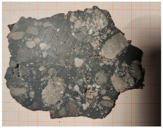
Figure 1.
Slab of the lunar meteorite NWA13859. The thickness of the slab is 2 ± 0.05 mm.
Clusters and fragments of light-toned minerals are well visible and are embedded in a dark matrix composed of glassy and/or microcrystalline materials. The weight of the sample is about 16.5 ± 0.3 g, which, coupled with the thickness of the sample and its surface, allowed us to derive a density of 2.4 ± 0.1 g/cm3. The density is calculated assuming no porosity in the rock. However, after a visual inspection of the cut slab (Figure 1), it is possible to observe small voids and vesicles. Therefore, the calculated density is assumed to be an upper limit of the actual density of the sample.
3. Methods
3.1. VNIR Measurements
A portable FieldSpec Pro spectrometer by Analytical Spectral Devices, Inc., was used to measure the reflectance spectra of the investigated samples in the spectral range 350–2500 nm. The spectral resolution was 3 nm in the visible region and 10 nm in the near infrared. The light source was a QTH (quartz–tungsten–halogen) lamp, and the radiation was delivered to the sample through an optical fiber. Another optical fiber was used to collect the signal reflected by the sample and direct it toward the spectrometer. The two optical fibers were mounted on a goniometer to control the experimental geometry, which was set to 30° for the incident angle and to 0° for the emission angle throughout the whole experimental session. An illustration of the setup is shown in Figure S1 (Supplementary Materials), and additional details are given in [15]. To calibrate the reflectance, we used a 99% reflectance Spectralon (Labsphere ®) standard. During the measurement, the sample was lying above a motorized stage. Two stepper motors allowed for moving the sample in the X and Y directions with a minimum sampling step of 0.5 mm. The height of the sample with respect to the focal point of the illumination spot was adjusted with a screw, whose minimum step was 5 µm. To check for instrument stability during the transect and map measurements, we repeated a measurement on a given point after about 20 min of operation. Three stability tests were executed during the transect and map data acquisition, and they showed no significant spectral drift during the 20 min of measurements. Therefore, we repeated the calibration of the instrument and the collection of the reference spectrum after every 20 min of operation. To avoid specular reflection and consequent loss of signal, we analyzed the rougher surface being more prone to diffuse scattering. The acquired spectra were continuum removed, and the band parameters were calculated (see Supplementary Materials Figure S2 and Equations (S1)–(S3)).
3.2. Endmember Measurements
Based on a visual inspection of the meteorite, we selected 16 representative spots on which we performed point analysis with the aim of catching the spectral heterogeneity of the samples. The selected points were scattered all over the surface of the meteorite and can be visualized in Figure 2. Given the spatial resolution of our setup and the marked heterogeneity of the sample, the “endmembers” were actually composed of two or more distinct phases. All endmember spectra are shown in Figure S3 (supplementary Materials).
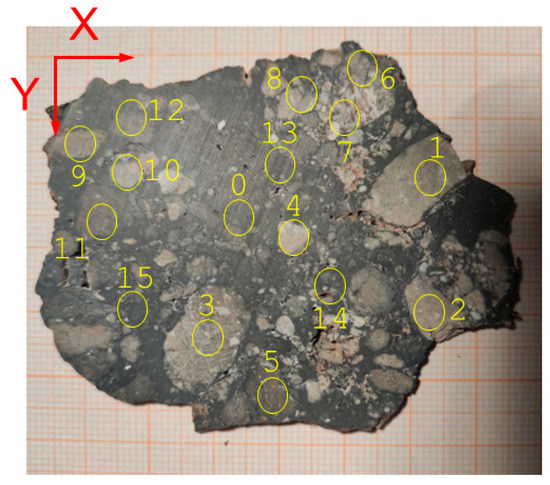
Figure 2.
Position of the analyzed spots (endmembers) on NWA 13859. The ellipses mark the analyzed spots, and the sequential numbers (0 to 14) identify each spectrum. The position of the orthogonal reference axes (X and Y) is marked by red arrows.
3.3. Transect Measurements
For the transect analysis, we acquired 24 spectra between EM_#1 and the matrix to its side. The origin of the new axis system is approximately centered on EM_#1 and is shifted and rotated clockwise at 42 degrees with respect to the coordinate system used for the EMs analysis and the grid analysis. Half of the spectra were acquired along the Y = 0 mm line defined by the reference system defined in Figure 3 (further details are shown in Figure S4 of the Supplementary Materials). The other 13 spectra were acquired along Y = 1 mm. Along the X-axis, consecutive spectra were separated by 1 mm, which means that consecutive measurements overlapped with each other by 80%. A similar approach was successfully applied by [15], to model the reflectance properties of an olivine–diogenite meteorite sample: they produced a transect between a mm-sized olivine clast and the surrounding rock and described the reflectance properties along the transect.
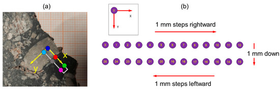
Figure 3.
Position and characteristics of the transect. (a) Position of the transect on the slab. Colored dots correspond to the positions of the spectra acquired on EM_#0 (blue and light blue), transition zone (red and gray), and matrix (green and fuchsia). (b) Position of each spectrum acquired along the transect. X- and Y-axes are also indicated. The orthogonal reference system used in the transect is rotated 45 clockwise with respect to the one used for the endmember analysis. Each spectrum is collected along the X-axis at 1 mm from the previous one. The spectra from 0 to 12 are acquired at Y = 0 mm.
3.4. Grid Measurements
For the grid measurements, we focused on a portion of the meteorite characterized by a prominent mineralogical heterogeneity. The investigated surface had an area of 8.58 cm2. The measurements were performed on a grid composed of 15 points along the X-axis and 5 points along the Y-axis. The points were regularly spaced along the two axes. The distance between consecutive measurements was 2 mm along the X-axis and 5 mm along the Y-axis. A scheme of the measured area with analytical details is presented in Figure 4. The aim of the grid analysis is to simulate an imaging spectroscopy apparatus. However, there is a major difference between the approach proposed in point 3 and a proper imaging system: in an imaging system, each pixel of the detector collects the light from a specific area of the sample, while in our approach, the measurements are partly superimposed to each other, leading to a redundancy of the data. In particular, consecutive measurements are expected to be very similar to each other with only minor variations in the spectral features. The minor variations observed between consecutive measurements are due to the signal coming from different portions of the sampled area. Therefore, they are representative of an area smaller than the typical spatial resolution of the instrument. Given the typical spatial resolution of our setup (between 5 and 6 mm) and the heterogeneity of the sample, a generic spectrum collected on the NWA13859 slab is likely the result of overlapping signals coming from different EMs. Therefore, we applied the strategy in point 3, attempting to increase the spatial resolution by oversampling the signal.
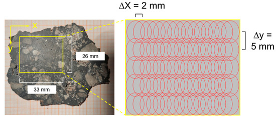
Figure 4.
Position and geometric features of the spectra measured on the densely spaced grid. The yellow square delimitates the area of the meteorites investigated with this methodology. X- and Y-axes are marked with arrows. Each spectrum is acquired at a distance of 2 mm from the previous one along the X-axis and 5 mm along the Y-axis. Red ellipses correspond to the illuminated area of each measurement spot.
4. Results and Discussion
4.1. Endmember Analysis
Despite the large number of spectra collected on the slab and the mineralogical complexity of the sample, most of the spectra look quite similar with minor variations in band shape, position, and area. Figure 5 shows some representative spectra on the EMs collected in step 1. Band I centers (BIC, namely, the minimum in reflectance after continuum removal of the band centered between 900 and 1100 nm) are found between 940 and 960 nm with the exception of EM_#0 characterized by a BIC of about 1100 nm.
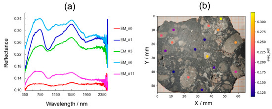
Figure 5.
Results of the endmember analysis. (a) Five representative spectra (EM_#0, EM_#1, EM_#3, EM_#6, and EM_#11 in Figure 2) of the sample NWA13859. (b) Position of the EMs on the X–Y reference axes defined in Figure 2 (the actual optical image is in the background of the plot). The colors of the points represent the average reflectance (average reflectance value between 500 and 1000 nm).
The band centered at ~950 nm (BI) is quite broad and asymmetric, while the band centered at about 1900 nm (BII) is broader and shallower than BI. In the case of EM_#0 BII, it is barely resolvable. In EM_#1 and EM_#6, we observed a narrow 1930 nm band superimposed to a much broader and shallower band. Considering these spectral features, it is likely that the spectra are the result of overlapping contributions from different mineral phases: indeed, the position of BI and BII is consistent with orthopyroxenes (OPX), while the asymmetry of BI could be explained by hypothesizing the contribution from olivine (Ol), plagioclase (Pl) and Fe-bearing glass, clinopyroxene (CPX), or a combination of the four phases. A weak absorption band at 1930 nm is attributable to H2O vibrations and, hence, to partial terrestrial alteration (e.g., [16]). However, given the very small amplitude, it is negligible. According to Meteoritical Bulletin number 110, the content of OPX is very low in the discussed meteorite. In spite of that, it dominates the spectral features of the sample. In Figure 5b, we plotted the position of the analyzed spectra on the X–Y-axes. In this plot, the color of the points in panel (b) corresponds to the average reflectance between 500 and 1000 nm. This simple parameter can give insightful information about the different mineralogical content of the investigated spots. The EMs characterized by the highest reflectance correspond (as expected) to the phases characterized by bright appearance. EM_#0 corresponds to the matrix. Its spectrum is characterized by a low value of reflectance (as expected, given its dark hue), one broad, shallow, and almost symmetric band centered at 1100 nm, weak BII, and low spectral contrast. These features can be interpreted as the result of a mixture of Fe-bearing glass, olivine, and ilmenite [17,18,19,20]. EM_#1 appears as a composite clear clast (Figure 1) with some smaller and brighter inclusions (likely Pl). The average reflectance of this clast is much higher than EM_#0 but not as high as EM_#6. We hypothesize that the average reflectance is proportional to the plagioclase-to-mafic-mineral ratio. The main effect of plagioclase is to increase the reflectance values with only minor effects on the band position and shape.
4.2. Transect Analysis
Six representative spectra are plotted in Figure 6, which allow for inferring how spectral properties change along the transect. Along the Y = 0 mm line, we see a continuous decrease in the overall reflectance of the spectra accompanied by a marked shift of the 1 µm band center from lower to higher wavelength likely due to the combined effect of opaque phases in the matrix, higher olivine content, and presence of glassy materials. It is also worth discussing the variation of the 1 µm band shape and area and the disappearance of the 2 µm band from EM_#1 to the matrix.
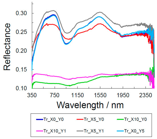
Figure 6.
Representative spectra acquired along the transect. The position where the spectra were acquired corresponds to the position shown in Figure 3a. Spectrum Tr_X0_Y0 (blue) was acquired at the origin of the reference system, while Tr_X0_Y5 (light blue) was acquired 5 mm along the Y-axis. Spectra Tr_X5_Y0 (red) and Tr_X5_Y1 (gray) were collected on the transition zone. Spectra Tr_X10_Y0 (green) and Tr_X10_Y1 (fuchsia) were collected on the matrix. Numbers after the “X” and the “Y” correspond to the values in mm of the X- and Y-axes where the spectra were acquired.
The 1 µm absorption is deep and asymmetric on EM_#1 while becoming much broader and shallower but also symmetric on the matrix. It is worth pointing out that the left shoulder of the band is found at a lower wavelength in the matrix. These spectral features support the hypothesis that the matrix is enriched in olivine (more symmetric band), ilmenite, and glass (lower reflectance, lower spectral contrast, and broader band). For the line at Y = 1 mm, the situation is similar to the previous one with regard to the end members. It is interesting to note that the spectra acquired at X = 5 mm and Y = 1 mm (grey) display the highest reflectance at all wavelengths but no significant variations in band shape and other spectral features with respect to the other spectra. These differences can be explained assuming the presence of a relatively featureless phase (which causes no significant variation in spectral features) and bright material (which causes the increase in reflectance). Plagioclase has these spectral characteristics [21], and therefore, we infer the presence of this mineral phase between EM_#1 and the matrix. Is it also worth discussing the fact that the spectra acquired at X = 5; Y = 0 (red) and X = 5; Y = 1 (gray) have a difference in reflectance of about 4%, but they are acquired at a distance of 1 mm along the Y-axis from each other. We further investigated the variation of the spectral parameters along the transect, and we summarized the results in Figure 7. We see that several parameters (band center and spectral slope) remain constant (within uncertainties) between 0 and 3 mm (from EM_#1) and between 7 and 12 mm. The BI area decreases from 0 to 7 mm and then increases up to 12 mm. The average reflectance increases linearly between 0 and 3 mm for Y = 0 mm. For Y = 1 mm, we observed a similar behavior, but the average reflectance increased up to 4 mm from EM_#1. This steady increase (about twice the magnitude of the error associated) of the average reflectance in the initial part of the transect is indeed very interesting: given the much lower reflectance of the matrix with respect to EM_#1, it would be expected to see a stationary value in the first 2 or 3 mm and then a drop in reflectance. As hypothesized before, the presence of a high-reflectance minerals (such as plagioclase) dispersed inside EM_#1 is a possible explanation of the observed parameter variation. A careful examination of Figure 1 reveals the presence of whitish mm-sized clasts (likely feldspars), which support our hypothesis. It is worth pointing out that, with such a procedure (partly superimposed consecutive measurements), it is possible to infer the presence of phases having a much smaller scale than the spatial resolution of our instrument.
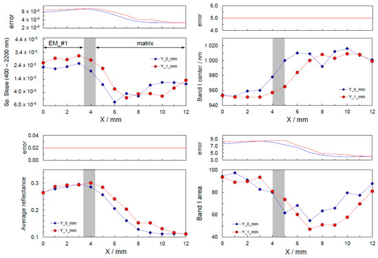
Figure 7.
Band 1 (~980 nm) measured parameters in the transect between EM_#1 and the matrix. Note that the error bars are not plotted for a clearer visualization of the results, but the calculated errors on band parameters are displayed in a separate panel on top of each plot. Area shaded in gray represents the transition boundary between EM_#1 and the matrix (about 1 mm thick of intermixed materials).
The highest rate of variation for all the parameters can be observed between 3 and 6–7 mm from EM_#1, which roughly coincides with the transition between EM_#1 and the matrix, which is located between 4 and 5 mm from the center of EM_#1. Between the two phases, there is about 1 mm of intermixed materials. It is important to remember that the spot size of our setup is about 5 mm × 6 mm (5 mm along the X-axis and 6 mm along the Y-axis).
We modeled the transition zone between EM_#1 and the matrix as being composed of 50% of phase 1 (EM_#1) and 50% of phase 2 (matrix). This assumption allows for the calculation of the area of EM_#1 and the matrix impinged by the light coming from the lamp and reflected to the spectrometer. Figure 8 depicts the transect model: PHASE 1 is EM_#1, PHASE 2 is the matrix, and PH1 (phase 1) + PH2 (phase 2) is the transition zone assumed to be composed of 50% (volume) EM_#1 and 50% matrix. The red oval (centered at X = 4; Y = 0) shows the geometry of the illuminated light spot on the sample’s surface. The plot shows the percentage of the area of the matrix illuminated by the light as a function of the light spot center along the transect. We can model the reflectance values along the transect, assuming a linear relationship between reflectance values of the two phases (EM_#1 and matrix) and assuming that their influence on the spectrum is linearly related to their respective area under the illuminated spot. First, we defined the reference reflectance spectrum of EM_#1 (REM1) as the average of the first two spectra for X = 0 and 1 mm and Y = 0 mm, while the reference reflectance spectrum for the matrix (Rmx) is the average of the last four spectra (X = 9, 10, 11 mm, and 12; Y = 0 mm).
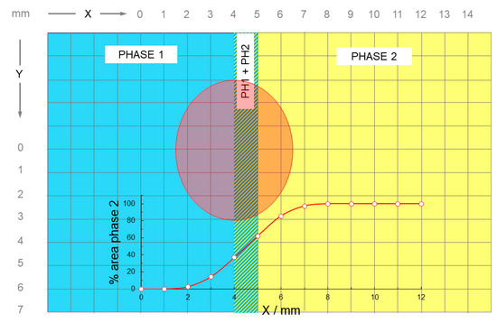
Figure 8.
Idealized and simplified model of the transect. PHASE 1 corresponds to EM_#0, while PHASE 2 corresponds to the matrix. Transition zone (PH1 + PH2) is modeled as 1 mm layers composed of 50% EM_#0 and 50% matrix. The red oval shows the area illuminated during a measurement. The graph on the bottom shows the percentage of PHASE 2 impinged by the light as a function of the position of the spotlight along the transect.
Equation (1) can be used to model the reflectance along the transect:
where Amx is the surface of the matrix (expressed as percentage) impinged by the light during the measurement. The values of Amx were calculated numerically and are reported in Table S1 in Supplementary Materials. It is worth specifying that Equation (1) is formally equivalent to Equations (1) and (2) proposed in [14], with the exception that the area here is expressed in percentage, while in [14], it is expressed as a unit fraction. Equation (1) is therefore a linear deconvolution model.
The spectra calculated with Equation (1) are reported in Figure 9 (panel (b)) and compared with the measured ones (panel (a)). From the comparison with the measured and the modeled spectra, we can see that the modeled spectra retain similarities with EM_#1, while in the measured spectra, the spectral contribution of the matrix is more evident. This could be due to the fact that the matrix is more efficient in determining the spectral features of the measured spectrum (which would imply a nonlinear mixing behavior of the two phases) or that the matrix is more abundant in the transition zone. We quantitatively evaluated the differences between the modeled and measured spectra by calculating the main spectral parameters (band I center, band I area, average reflectance (between 500 and 1000 nm) and spectral slope between 400 and 2200 nm), and the results are presented in Figure 10. The results are reasonable for the BI asymmetry (BS) and BI center (BC), but for BS, the model significantly overestimates the measured values, while for BC, the model underestimates the measured values along the transition zone. Both these observations are consistent with the hypothesis that the matrix is more effective in determining the spectral features with respect to EM_#1. With regard to the spectral slope (SS) and the BI area (BA), the model fails to reproduce the observed values. In particular, the model produces completely unreliable results for BA. The reason for such a discrepancy is likely the presence of additional phases at a mm or sub-mm scale in the investigated area.
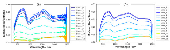
Figure 9.
Measured and modeled spectra for the transect (Y = 0). (a) Measured spectra. (b) Modeled spectra. Final numbers in the label refer to the X-position (mm) of the spectrum along the transect.
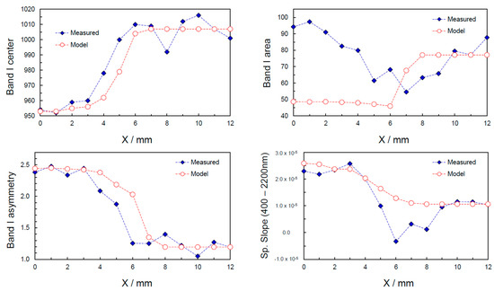
Figure 10.
Measured band parameters for the modeled spectra (red circles) and measured spectra (blue diamonds). Dotted lines connect the data point and are shown as a visual aid. Sp. Slope (400–2200 nm) is the spectral slope calculated between 400 and 2200 nm.
In addition to the linear model, we used the Spectral Angle Mapper (SAM; e.g., [22]) to quantitatively define the spectral differences between the matrix and EM_#1. We first calculated the SAM algorithm using phase 1 (matrix) as reference spectrum, and then we performed the calculation using phase 2 (EM_#1) as reference spectrum. The results are shown in Figure 11. When the spectrum of EM_#1 is taken as reference spectrum, we see a mild but steady increase in angle up to 5 mm, which is likely due to a mineralogical heterogeneity of EM_#1. From 5 to 11 mm, there is a stronger increase in angle, testifying a significant variation of the spectral parameters. This strong variation is due to the boundary between EM_#1 and the matrix. From 11 to 13 mm, we see no variation of the SAM angle, which means that after 11 mm, the SAM is not able to distinguish any difference in the spectra of the matrix relative to the spectrum of EM_#1. The situation is slightly different when the spectrum of the matrix is taken as reference spectrum. We observed a gradual decrease in the SAM values, which is likely attributable to the extreme mineralogical heterogeneity of the matrix.
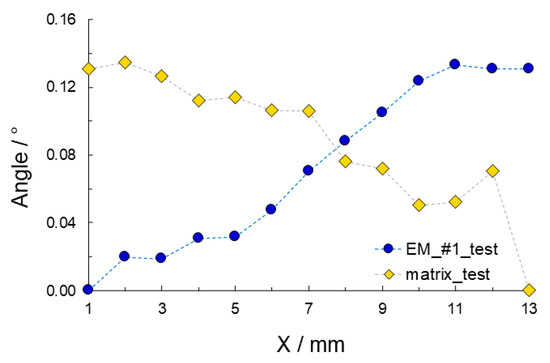
Figure 11.
Results of the Spectral Angle Mapper calculations for the transect. Blue circles are the results of the calculations with the spectrum of EM_#1 as reference spectrum, while yellow diamonds are the results of the calculations with the spectrum of the matrix as reference spectrum.
4.3. Array Analysis
The array analysis of the data acquired on the densely spaced grid allowed us to create detailed maps of the investigated surface, mimicking a hyperspectral image (further details about the maps’ creation are given in the Supplementary Materials—spectral maps section). Once again, it is interesting to note that the analytical strategy of performing partly superimposed adjacent measurements allowed us to resolve details with a higher spatial resolution of the instrument spot size, as shown in Figure 12. Panel (a) in Figure 12 shows the average reflectance between 500 and 1000 nm, which is relatively low throughout the investigated area. The low average reflectance in the VIS–NIR portion of the spectra can be attributed to the diffuse presence of olivine, glass, and opaque minerals such as ilmenite (e.g., [19,20]). The average reflectance marks very well the contrast between the clast and the matrix. This is not surprising since, as discussed in the case of endmember and transect analysis, the matrix is characterized by a low reflectance, while clasts have a markedly higher reflectance. However, the spatial resolution achieved with this technique is noteworthy. Similar maps are produced for the area of the band at 1 µm (BA I). BA I (panel (b) in Figure 12 is even more sensitive in assessing the mineralogical diversity of the sample as it is very useful in identifying the clasts within the matrix. Indeed, from a comparison with Figure 4, it is possible to see that the area characterized by high values of BA corresponds with the whitish clasts. The center of the band at 1 µm (BC I) has a maximum value (~1120 nm) around X = 22 mm and Y = 16 mm (Figure 12c), which approximately correspond with EM_#4 (Figure 2). However, our approach allowed us to restrict the portion of the slab in which BC I shows a value higher than 1110 nm. Such area (≈2 mm × 2 mm) corresponds with the upper-left portion of EM_#4, which is characterized by a whitish and bright appearance. Similarly, the lowest values of BC I correspond with the highest values of average reflectance in panel (a), which, given the low values of BC I, we associate with orthopyroxenes [23]. It is surprising to see how a supposedly minor phase like orthopyroxene dictates the spectral behavior in some areas of the sample. In panel (d) of Figure 12, we plot the SS (spectral slope calculated between 400 and 2200 nm). SS is generally low and even negative, reaching the minimum value (−0.8 × 10⁻⁵) in the matrix. Higher SS values can be found in the clast between 3 < X < 10 mm and 0 < Y < 13 mm. It is not unclear how to interpret the highest SS value found at X = 24; Y = 20. The maximum SS point roughly corresponds with EM_#4, but it is slightly shifted with respect to the maximum values of BC I and average reflectance. We also point out the sharp spatial gradient of SS associated with this maximum.
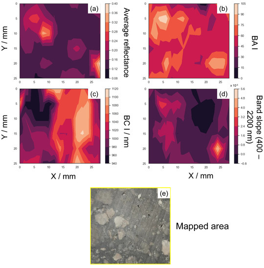
Figure 12.
Spectral parameter maps of NWA 13859. Panel (a) shows the average reflectance (average reflectance value between 500 and 1000 nm). Panel (b) shows the band area of band I (BA I, the band roughly centered at 1 µm). Panel (c) shows the band center of band I (the band roughly centered at 1 µm), panel (d) shows the spectral slope calculated between 400 nm and 2200 nm, while panel (e) at the bottom of the picture shows the mapped area. Horizontal axes represent X direction in mm, while vertical axes represent Y direction in mm.
5. Conclusions
We give the first spectroscopic characterization of the NWA 13859 lunar feldspathic breccia. Our preliminary results show a dominant effect of orthopyroxene on the spectral features of the clasts, while the matrix has spectral features that can be associated with a mixture of Fe-bearing glasses, olivine, and opaque materials (ilmenite). An in-depth spectral analysis of the transect (measured between a clast and the matrix) and the comparison with a linear deconvolution model (Equation (1)) gives unsatisfactory results. The disagreement of the observed and modeled results is in part due to an oversimplified linear model and in part to a complex mineralogy (presence of other mineral phases, chemical diffusion) of the transition zone between the two endmembers. We developed a methodology to obtain 2D spectral maps of a sample’s surface having a higher spatial resolution than the instrument’s spot size. Upon comparison of different spectral parameter maps of the same surface, the methodology proved to be effective in discriminating the different mineral phases. After additional tests and validation, this methodology can also be applied to remotely sensed data and, therefore, is of high relevance for both meteorite and planetary surface mineralogical studies.
Supplementary Materials
The following supporting information can be downloaded at https://www.mdpi.com/article/10.3390/min13081000/s1, Figure S1: Setup description, Figure S2: band parameters, Figure S3: End-member spectra; Figure S4: Details of the transect measurements; Table S1: Area of matrix impinged by the light (transect).
Author Contributions
Conceptualization, E.B., C.C. and F.T.; methodology, E.B. and C.C.; software, E.B.; validation, E.B.; formal analysis, E.B.; investigation, E.B. and C.C.; resources, F.T.; data curation, E.B.; writing—original draft preparation, E.B.; writing—review and editing, E.B., C.C. and F.T.; visualization, E.B.; supervision, C.C. and F.T.; project administration, F.T.; funding acquisition, F.T. All authors have read and agreed to the published version of the manuscript.
Funding
We acknowledge the support from the PRIN INAF (RIC) 2019 project “MELODY: Moon multisEnsor and LabOratory Data analYsis”, selected by the Scientific Direction of Italy’s National Institute for Astrophysics (INAF) on 10 November 2020 and funded with EUR 167,162 (INAF grant 1.05.01.85.17).
Data Availability Statement
All the spectra discussed in this work can be found as Supplementary Materials along with details about the experimental procedure.
Acknowledgments
The authors are grateful to the reviewers for their suggestions and comments, which allowed them to improve this manuscript.
Conflicts of Interest
The authors declare no conflict of interest.
References
- Mckay, D.S.; Morrison, D.A. Lunar breccias. J. Geophys. Res. 1971, 76, 5658–5669. [Google Scholar] [CrossRef]
- Korotev, R.L.; Zeigler, R.A.; Jolliff, B.L.; Irvin, A.J.; Bunch, T.E. Compositional and lithological diversity among brecciated lunar meteorites of intermediate iron concentration. Meteorit. Planet. Sci. 2009, 44, 1287–1322. [Google Scholar] [CrossRef]
- Collareta, A.; D’Orazio, M.; Gemelli, M.; Pack, A.; Folco, L. High crustal diversity preserved in the lunar meteorite Mount DeWitt 12007 (Victoria Land, Antarctica). Meteorit. Planet. Sci. 2016, 51, 351–371. [Google Scholar] [CrossRef]
- Stephant, A.; Anand, M.; Ashcroft, H.; Zhao, X.; Hu, S.; Korotev, R.; Strekopytov, S.; Greenwood, R.; Humphreys-Williams, E.; Liu, Y.; et al. An ancient reservoir of volatiles in the Moon sampled by lunar meteorite Northwest Africa 10989. Geochim. Cosmochim. Acta 2019, 266, 163–183. [Google Scholar] [CrossRef]
- Agrell, S.O.; Scoon, J.H.; Muir, I.D.; Long, J.V.P.; McConnell, J.D.C.; Peckett, A. Mineralogy and petrology of some lunar samples. Science 1970, 167, 583–586. [Google Scholar] [CrossRef]
- Korotev, R.L.; Jolliff, B.L.; Zeigler, R.A.; Gillis, J.J.; Haskin, L.A. Feldspathic lunar meteorites and their implications for compositional remote sensing of the lunar surface and the composition of the lunar crust. Geochim. Cosmochim. Acta 2003, 67, 4895–4923. [Google Scholar] [CrossRef]
- Righter, K.; Collins, S.J.; Brandon, A.D. Mineralogy and petrology of the LaPaz Icefield lunar mare basaltic meteorites. Meteorit. Planet. Sci. 2005, 40, 1703–1722. [Google Scholar] [CrossRef]
- Klima, R.L.; Pieters, C.M.; Boardman, J.W.; Green, R.O.; Head, J.W.; Isaacson, P.J.; Mustard, J.F.; Nettles, J.W.; Petro, N.E.; Staid, M.I.; et al. New insights into lunar petrology: Distribution and composition of prominent low-Ca pyroxene exposures as observed by the Moon Mineralogy Mapper (M3). J. Geophys. Res. Planets 2011, 116, E00G06. [Google Scholar] [CrossRef]
- Taylor, S.R. Lunar Science: A Post-Apollo View: Scientific Results and Insights from the Lunar Samples; Elsevier: Amsterdam, The Netherlands, 2016. [Google Scholar]
- Che, X.; Nemchin, A.; Liu, D.; Long, T.; Wang, C.; Norman, M.D.; Joy, K.H.; Tartese, R.; Head, J.; Jolliff, B.; et al. Age and composition of young basalts on the Moon, measured from samples returned by Chang’e-5. Science 2021, 374, 887–890. [Google Scholar] [CrossRef] [PubMed]
- Tartèse, R.; Anand, M.; Gattacceca, J.; Joy, K.H.; Mortimer, J.I.; Pernet-Fisher, J.F.; Russell, S.; Snape, J.F.; Weiss, B.P. Constraining the evolutionary history of the Moon and the inner solar system: A case for new returned lunar samples. Space Sci. Rev. 2019, 215, 54. [Google Scholar] [CrossRef]
- Tompkins, S.; Pieters, C.M. Spectral characteristics of lunar impact melts and inferred mineralogy. Meteorit. Planet. Sci. 2010, 45, 1152–1169. [Google Scholar] [CrossRef]
- Gattacceca, J.; McCubbin, F.M.; Grossman, J.; Bouvier, A.; Chabot, N.L.; D’Orazio, M.; Goodrich, C.; Greshake, A.; Gross, J.; Komatsu, M.; et al. The Meteoritical Bulletin, No. 110. Meteorit. Planet. Sci. 2022, 57, 2102–2105. [Google Scholar] [CrossRef]
- Hiroi, T.; Kaiden, H.; Misawa, K.; Niihara, T.; Kojima, H.; Sasaki, S. Visible and near-infrared spectral survey of Martian meteorites stored at the National Institute of Polar Research. Polar Sci. 2011, 5, 337–344. [Google Scholar] [CrossRef]
- Carli, C.; Pratesi, G.; Moggi-Cecchi, V.; Zambon, F.; Capaccioni, F.; Santoro, S. Northwest Africa 6232: Visible–near infrared reflectance spectra variability of an olivine diogenite. Meteorit. Planet. Sci. 2018, 53, 2228–2242. [Google Scholar] [CrossRef]
- Clark, R.N.; Rencz, A.N. Spectroscopy of rocks and minerals, and principles of spectroscopy. Man. Remote Sens. 1999, 3, 3–58. [Google Scholar]
- Sunshine, J.M.; Pieters, C.M. Determining the composition of olivine from reflectance spectroscopy. J. Geophys. Res. Planets 1998, 103, 13675–13688. [Google Scholar] [CrossRef]
- Isaacson, P.J.; Pieters, C.M. Deconvolution of lunar olivine reflectance spectra: Implications for remote compositional assessment. Icarus 2010, 210, 8–13. [Google Scholar] [CrossRef]
- Stockstill-Cahill, K.R.; Blewett, D.T.; Cahill, J.T.; Denevi, B.W.; Lawrence, S.J.; Coman, E.I. Spectra of the Wells lunar glass simulants: New old data for reflectance modeling. J. Geophys. Res. Planets 2014, 119, 925–940. [Google Scholar] [CrossRef]
- Izawa, M.R.; Applin, D.M.; Morison, M.Q.; Cloutis, E.A.; Mann, P.; Mertzman, S.A. Reflectance spectroscopy of ilmenites and related Ti and TiFe oxides (200 to 2500 nm): Spectral–compositional–structural relationships. Icarus 2021, 362, 114423. [Google Scholar] [CrossRef]
- Serventi, G.; Carli, C.; Sgavetti, M.; Ciarniello, M.; Capaccioni, F.; Pedrazzi, G. Spectral variability of plagioclase–mafic mixtures (1): Effects of chemistry and modal abundance in reflectance spectra of rocks and mineral mixtures. Icarus 2013, 226, 282–298. [Google Scholar] [CrossRef]
- Kruse, F.A.; Lefkoff, A.B.; Boardman, J.W.; Heidebrecht, K.B.; Shapiro, A.T.; Barloon, P.J.; Goetz, A.F.H. The spectral image processing system (SIPS)—Interactive visualization and analysis of imaging spectrometer data. Remote Sens. Environ. 1993, 44, 145–163. [Google Scholar] [CrossRef]
- Cloutis, E.A.; Gaffey, M.J.; Jackowski, T.L.; Reed, K.L. Calibrations of phase abundance, composition, and particle size distribution for olivine-orthopyroxene mixtures from reflectance spectra. J. Geophys. Res. Solid Earth 1986, 91, 11641–11653. [Google Scholar] [CrossRef]


Disclaimer/Publisher’s Note: The statements, opinions and data contained in all publications are solely those of the individual author(s) and contributor(s) and not of MDPI and/or the editor(s). MDPI and/or the editor(s) disclaim responsibility for any injury to people or property resulting from any ideas, methods, instructions or products referred to in the content. |
© 2023 by the authors. Licensee MDPI, Basel, Switzerland. This article is an open access article distributed under the terms and conditions of the Creative Commons Attribution (CC BY) license (https://creativecommons.org/licenses/by/4.0/).