


Cross-Hole and Vadose-Zone Infiltration Tracer Test Analyses to Determine Aquifer Reactive Transport Parameters at a Former Uranium Mill Site (Grand Junction, Colorado)

 ,
, 
Abstract
1. Introduction
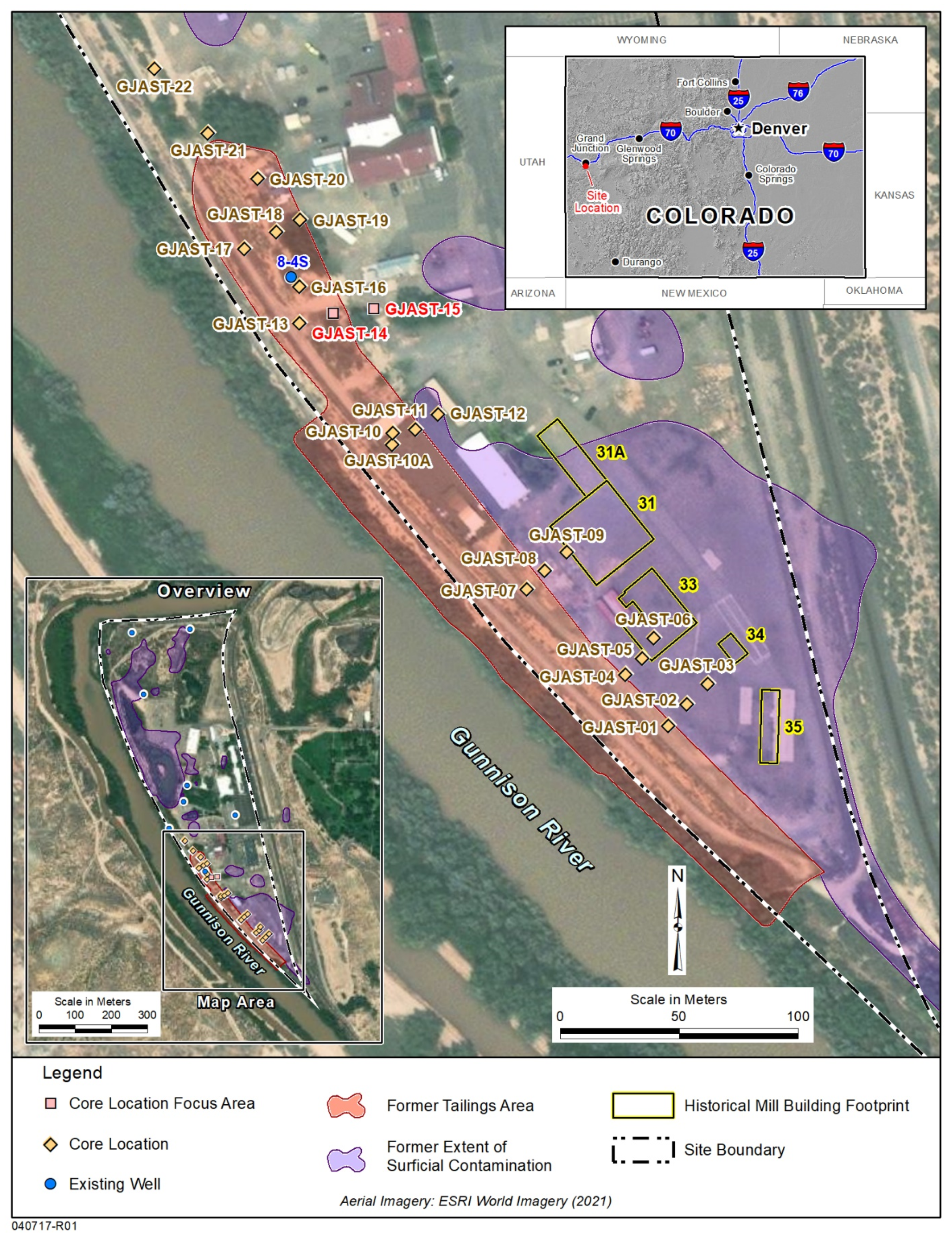
2. Site Background
3. Methods
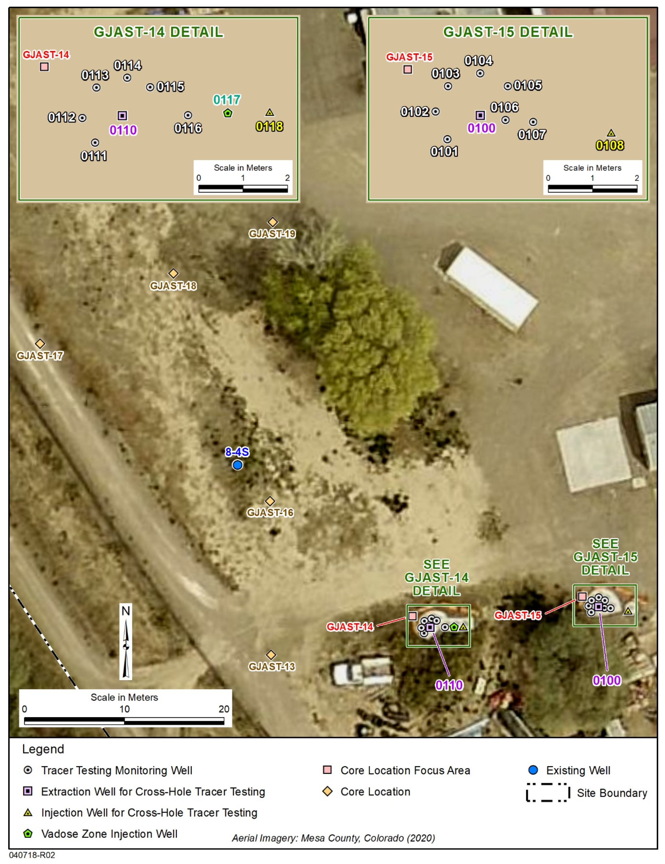
3.1. Well Installations and Flow Patterns
3.2. Tracer Testing Procedures
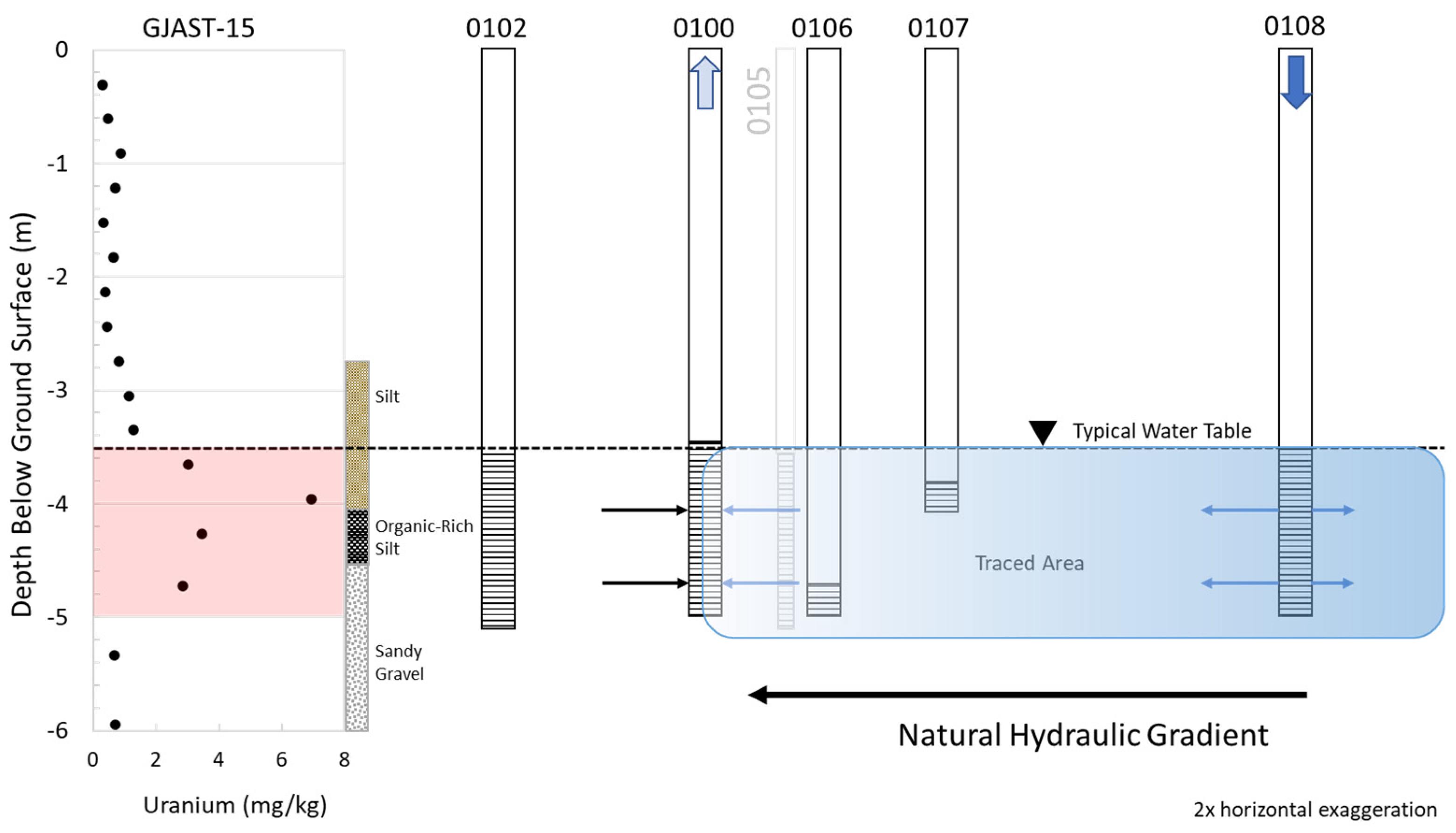
3.2.1. 100-Series Wells
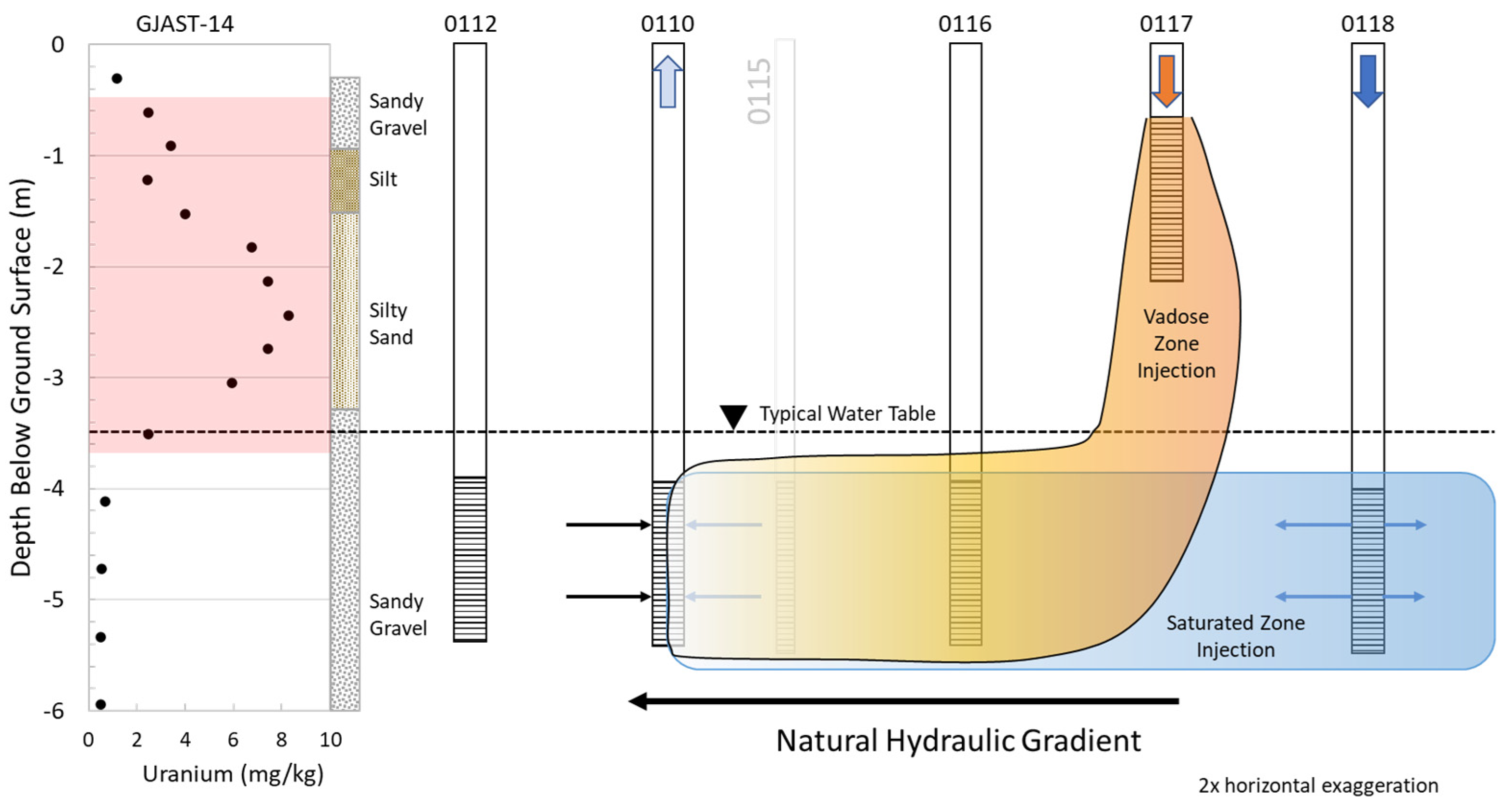
3.2.2. 110-Series Wells
3.3. Sampling and Analyses
3.4. Geochemical Modeling
3.5. Reactive Transport Modeling
4. Results and Discussion
4.1. Initial Groundwater and Surface Water Geochemistry
4.2. 100-Series Cross-Hole Saturated Zone
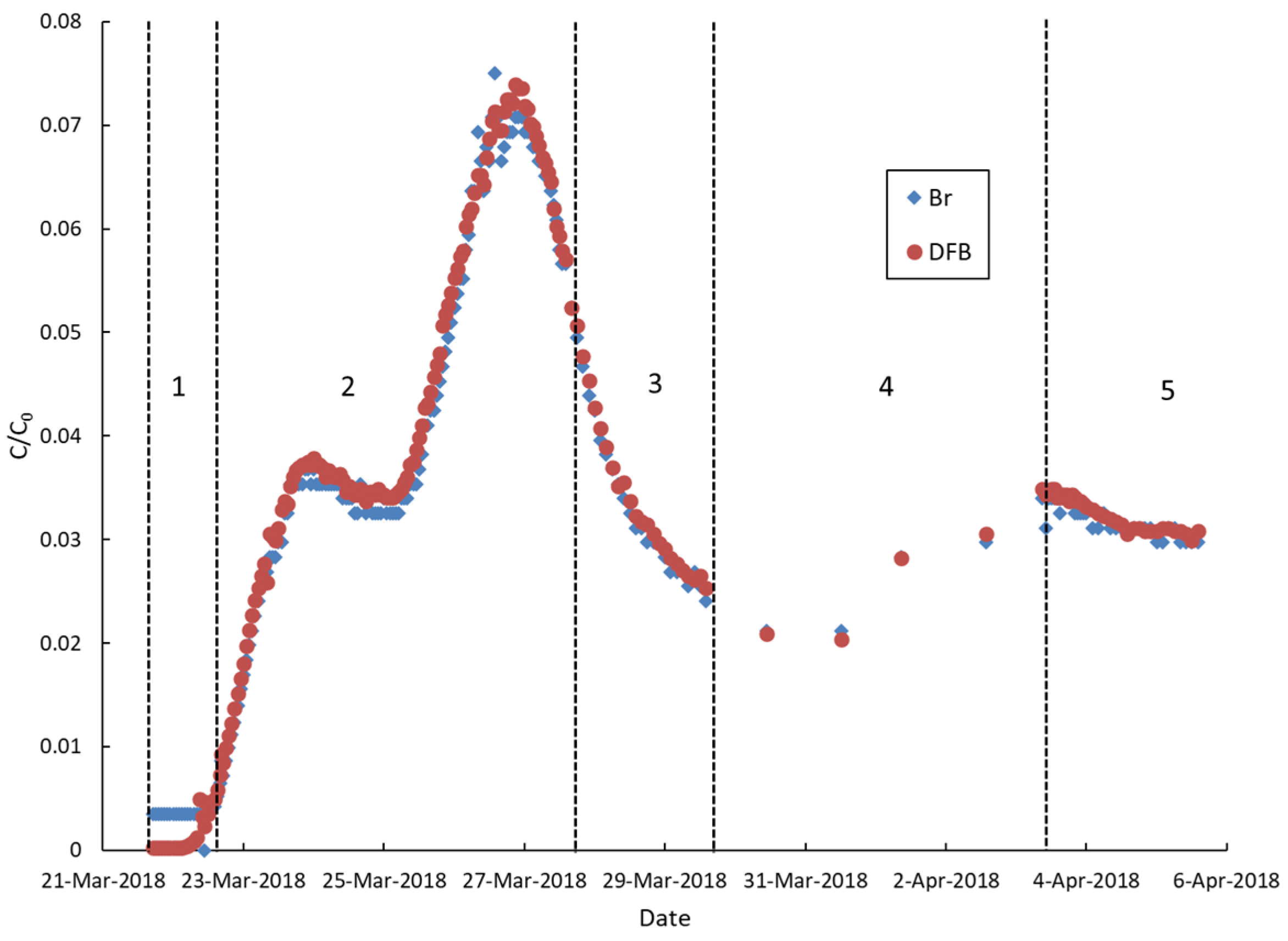
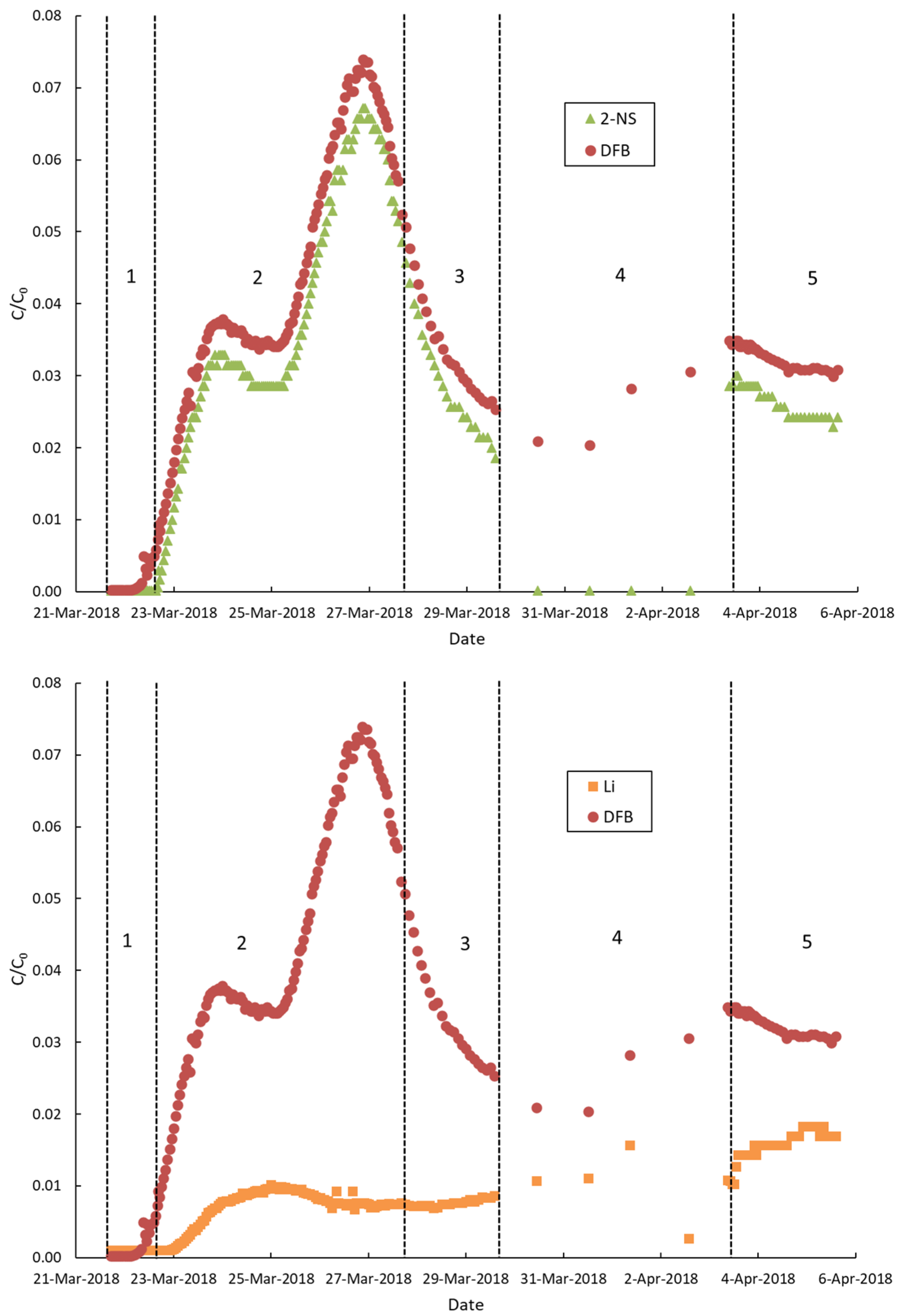
4.2.1. Tracer Results
4.2.2. Modeling Results
4.3. 110-Series Cross-Hole Saturated Zone and Infiltration
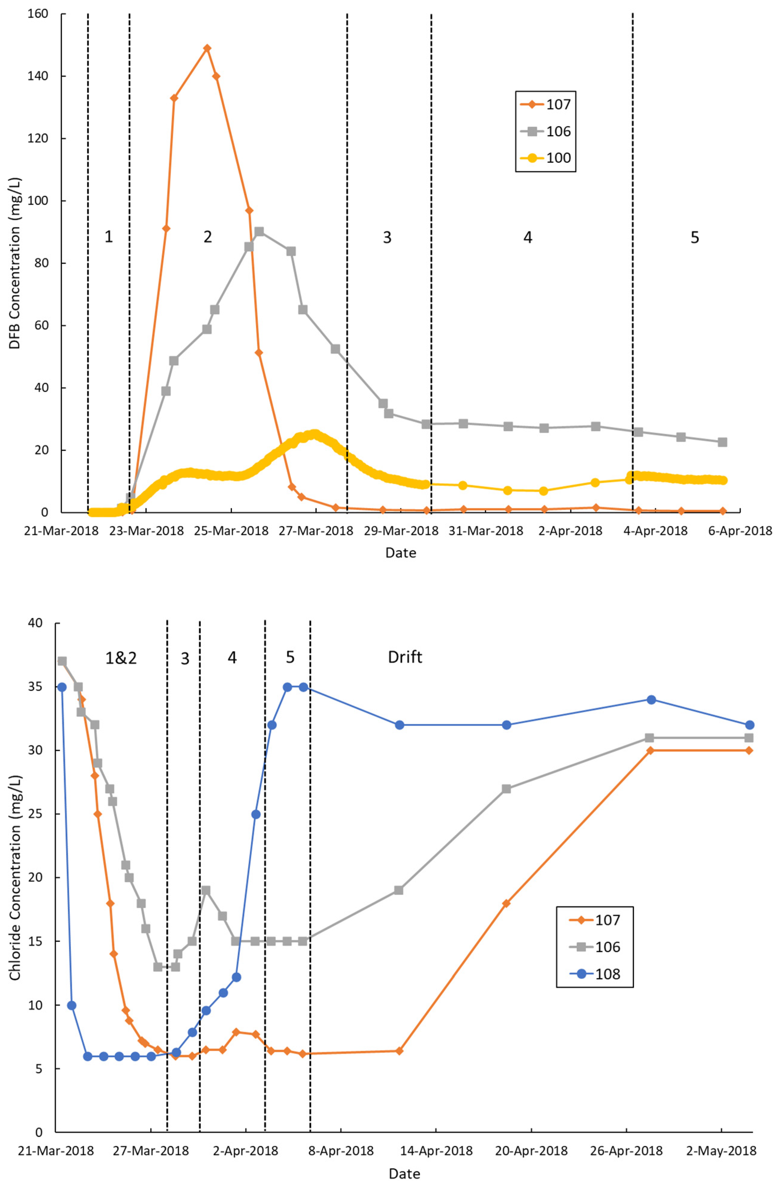
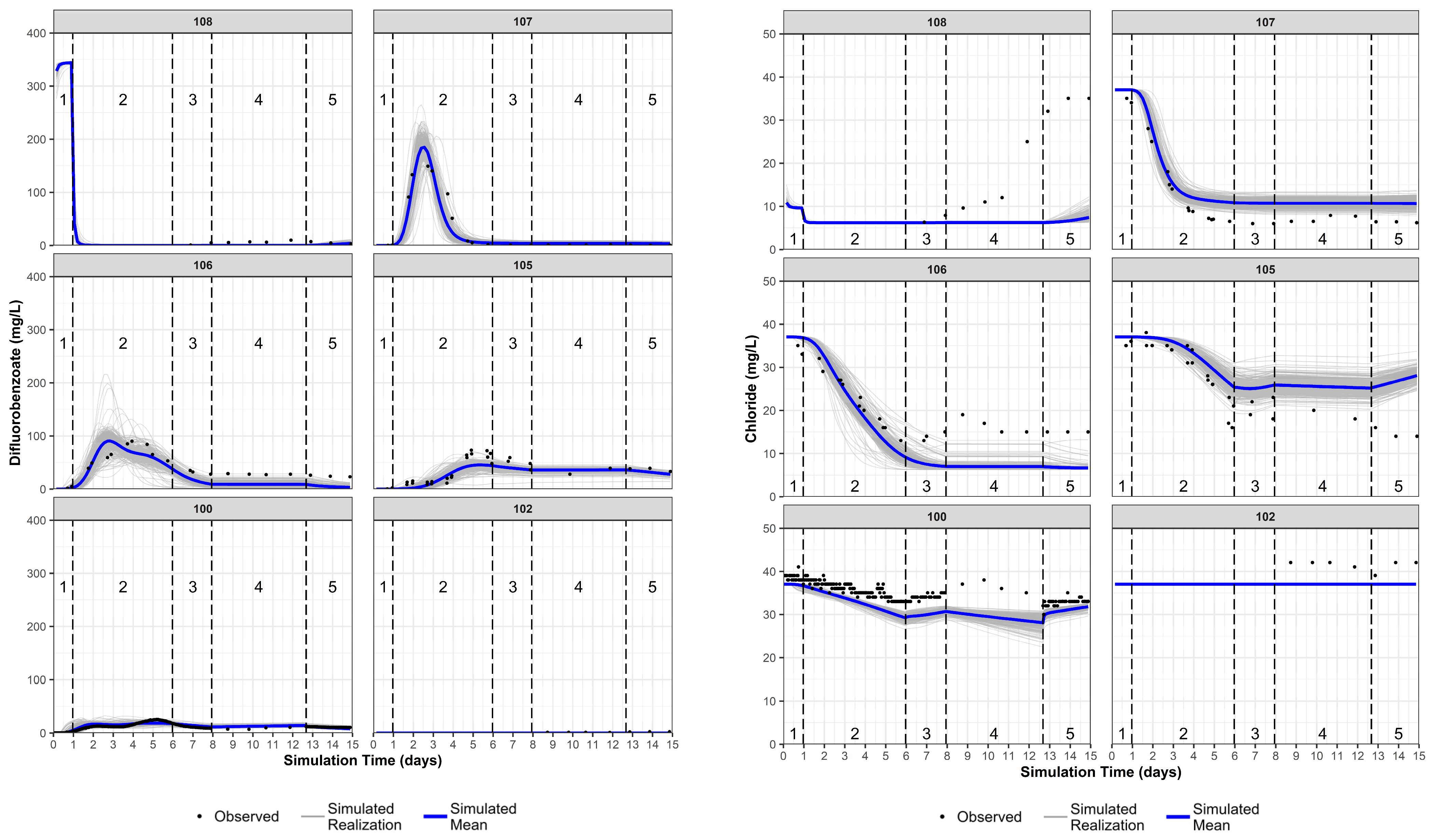
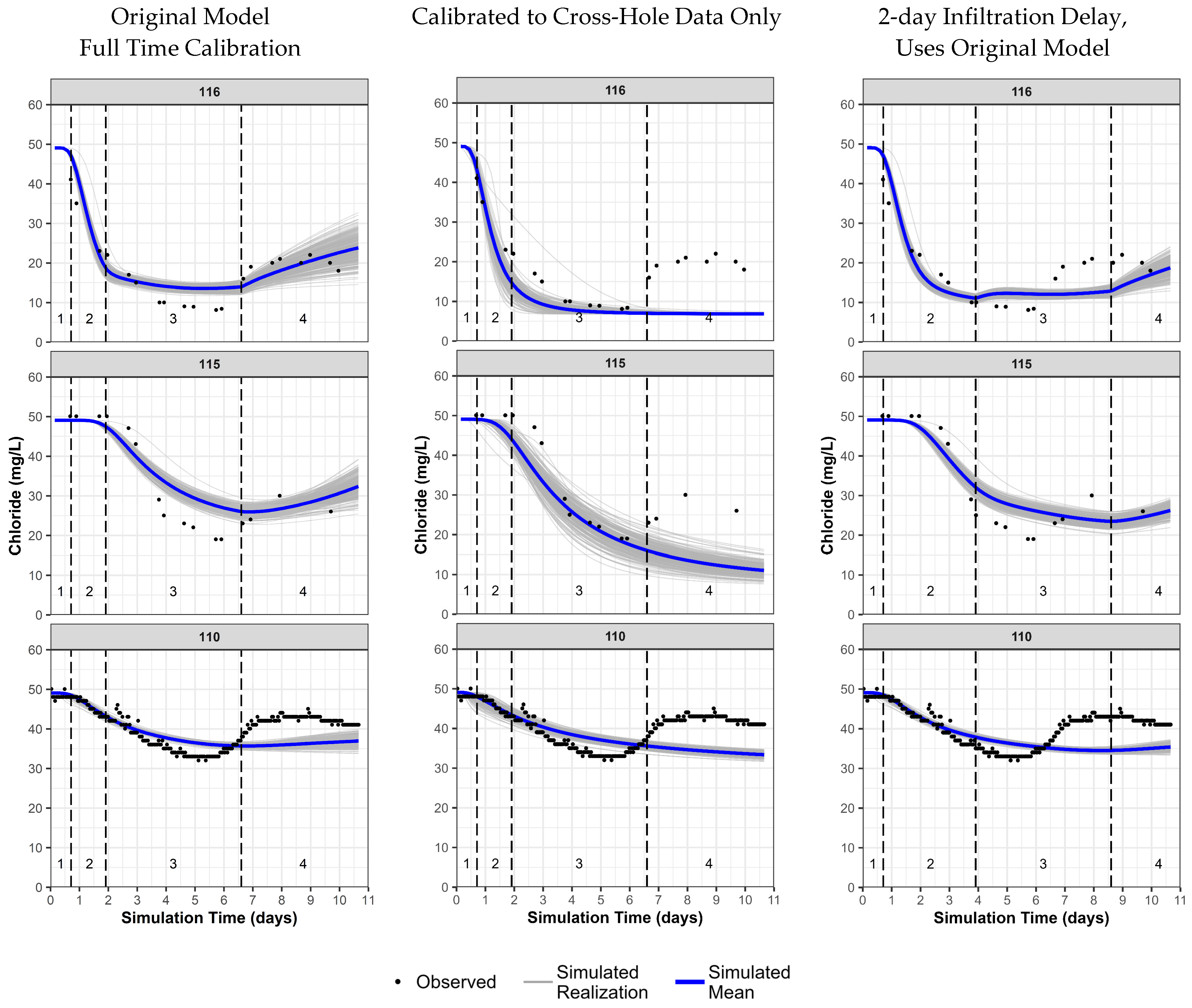
4.3.1. Tracer and Chloride Results
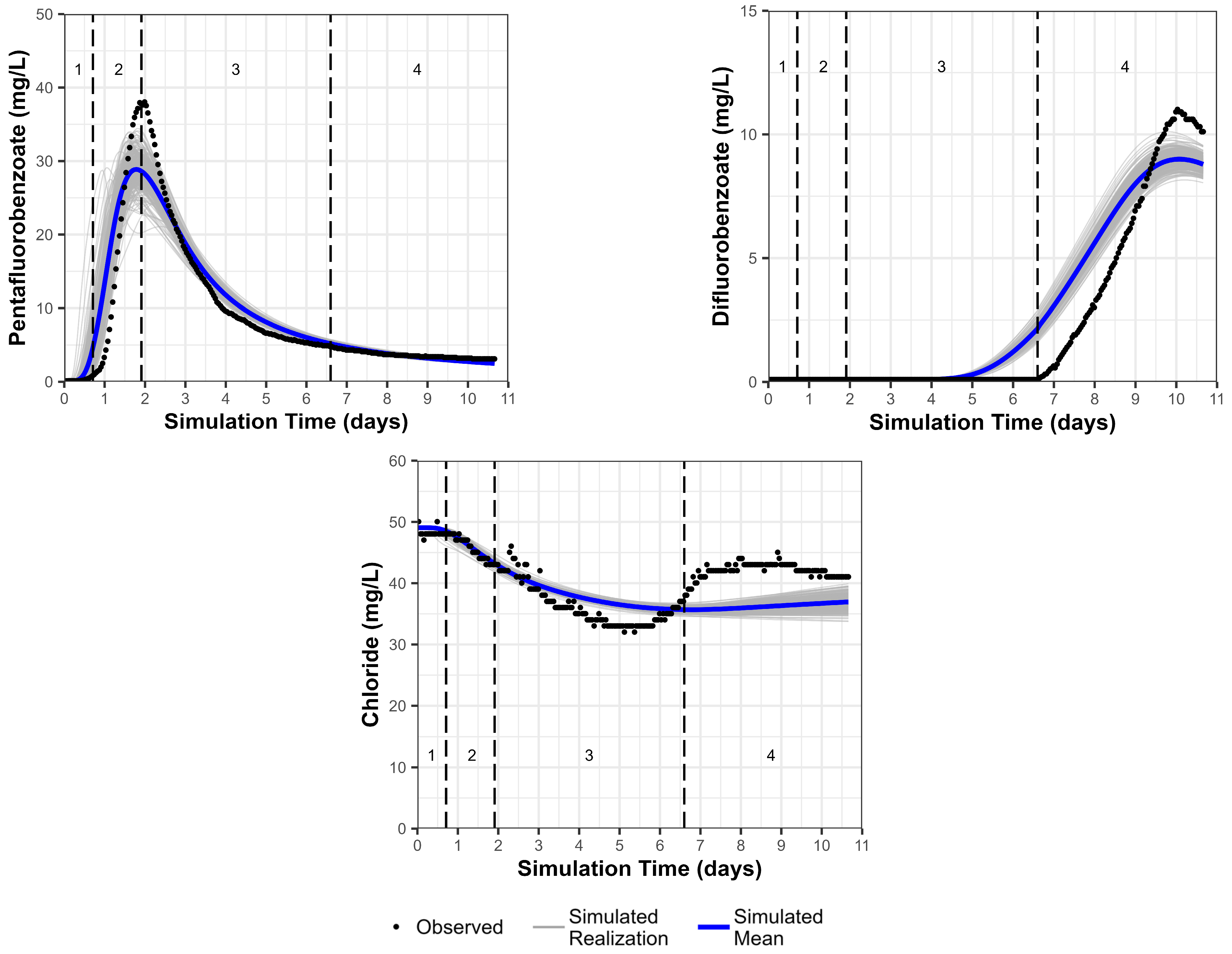
- Would calibrating to the cross-hole data only (days 0 to 5.7 before chloride concentrations increase from infiltration) improve simulated chloride concentrations from days 3 to 5.7 and result in any estimated parameter changes?
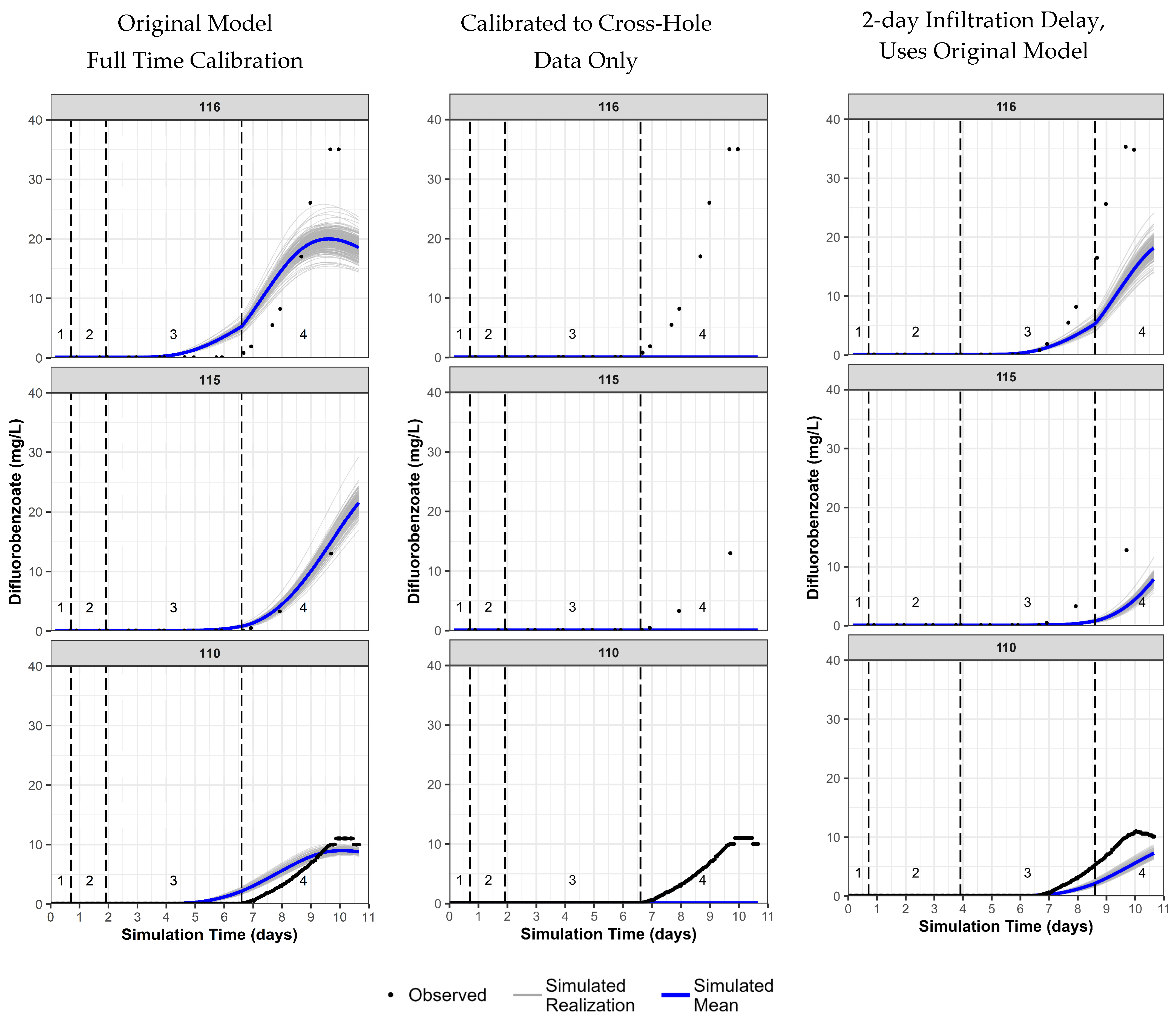
- Would a 2-day delay in infiltration timing create better simulated results for DFB?
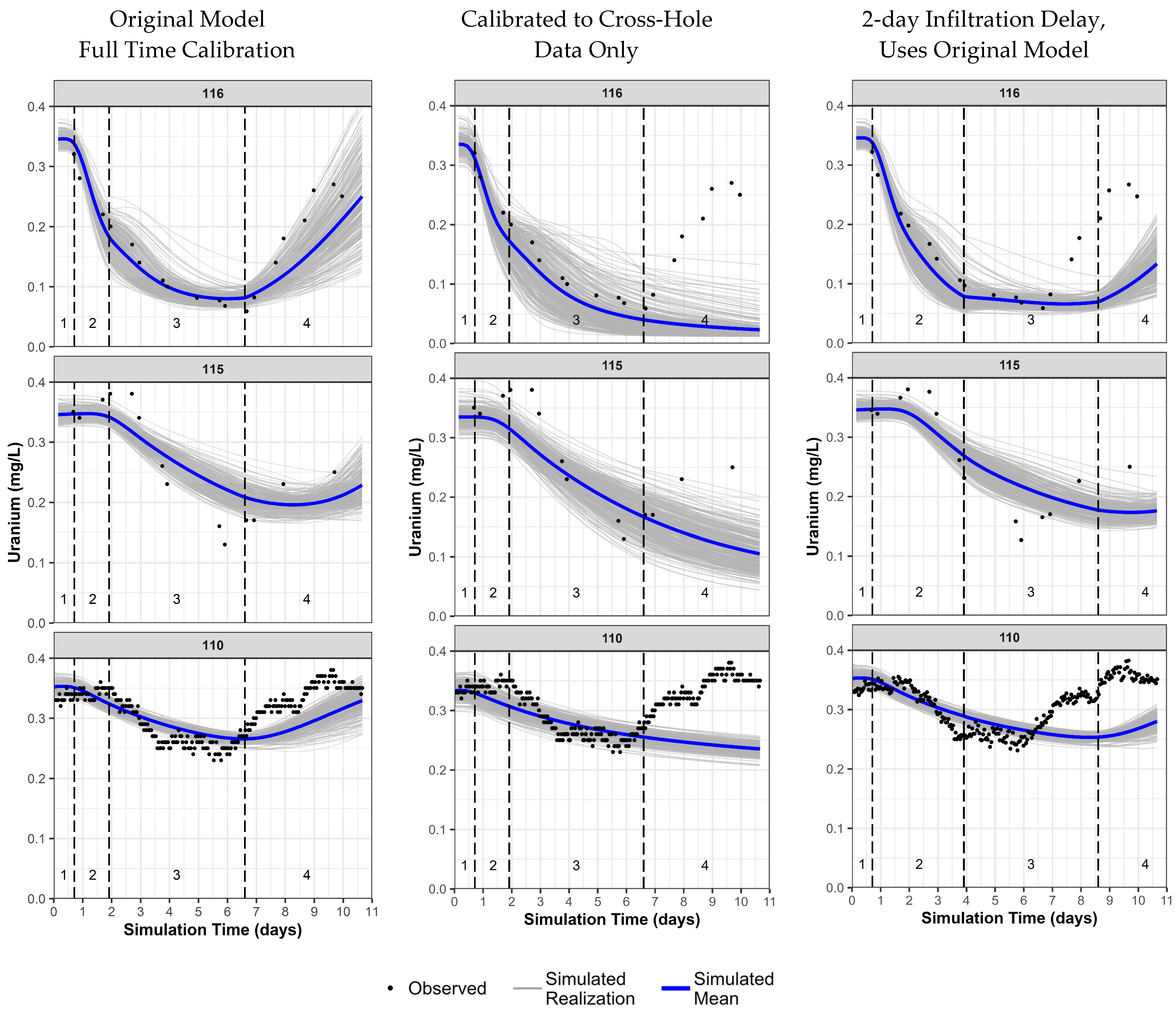
4.3.2. Additional Modeling
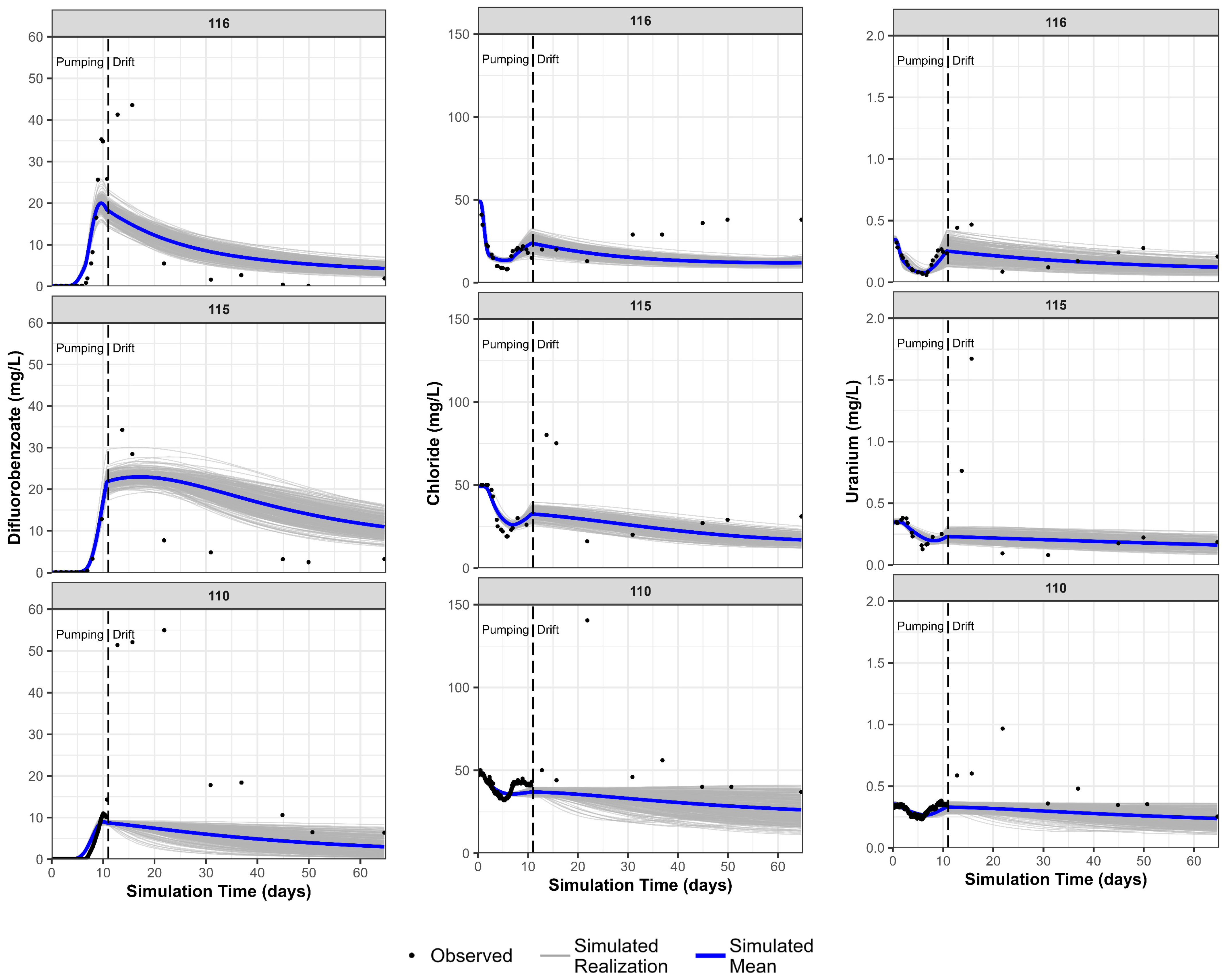
4.3.3. Final Drift Phase
4.4. Summary of Estimated Parameters
4.4.1. Physical Parameters
4.4.2. Geochemical Parameters
5. Conclusions
Supplementary Materials
Author Contributions
Funding
Data Availability Statement
Conflicts of Interest
References
- Dam, W.L.; Campbell, S.; Johnson, R.H.; Looney, B.B.; Denham, M.E.; Eddy-Dilek, C.A.; Babits, S.J. Refining the site conceptual model at a former uranium mill site in Riverton, Wyoming, USA. Environ. Earth Sci. 2015, 74, 7255–7265. Available online: http://link.springer.com/article/10.1007%2Fs12665-015-4706-y (accessed on 23 March 2023). [CrossRef]
- DOE (U.S. Department of Energy). Plume Persistence Final Project Report; LMS/ESL/S15233, ESL-RPT-2018-02; Office of Legacy Management: Grand Junction, CO, USA, 2018. Available online: https://www.energy.gov/lm/services/applied-studies-and-technology-ast/ast-reports (accessed on 23 March 2022).
- DOE (U.S. Department of Energy). Monticello Mill Tailings Site Operable Unit III Groundwater Flow and Contaminant Transport Model Report; LMS/MNT/S30707; Office of Legacy Management: Grand Junction, CO, USA, 2021. [Google Scholar]
- DOE (U.S. Department of Energy). Riverton, Wyoming, Processing Site: 2020 Geochemical Assessment Report; LMS/RVT/S36212; Office of Legacy Management: Grand Junction, CO, USA, 2022. [Google Scholar]
- Johnson, R.H.; Paradis, C.J.; Kent, R.D.; Tigar, A.D.; Reimus, P.W. Single-well push-pull tracer test analyses to determine aquifer reactive transport parameters at a former uranium mill site (Grand Junction, Colorado). Minerals 2023, 13, 228. [Google Scholar] [CrossRef]
- Paradis, C.J.; Johnson, R.H.; Tigar, A.D.; Sauer, K.B.; Marina, O.C.; Reimus, P.W. Field experiments of surface water to groundwater recharge to characterize the mobility of uranium and vanadium at a former mill tailing site. J. Contam. Hydrol. 2020, 229, 103581. [Google Scholar] [CrossRef]
- Johnson, R.H.; Tigar, A.D.; Richardson, C.D. Column-test data analyses and geochemical modeling to determine uranium reactive transport parameters at a former uranium mill site (Grand Junction, Colorado). Minerals 2022, 12, 438. [Google Scholar] [CrossRef]
- Reimus, P.W.; Arnold, B.W. Evaluation of multiple tracer methods to estimate low groundwater flow velocities. J. Contam. Hydrol. 2017, 199, 1–13. [Google Scholar] [CrossRef] [PubMed]
- DOE (U.S. Department of Energy). Fact Sheet for the Grand Junction, CO, Site; Office of Legacy Management: Grand Junction, CO, USA, 2022. Available online: https://www.energy.gov/lm/articles/grand-junction-colorado-site-fact-sheet (accessed on 23 March 2023).
- DOE (U.S. Department of Energy). Final Remedial Investigation/Feasibility Study for the U.S. Department of Energy Grand Junction (Colorado) Projects Office Facility; DOE/ID/12584-16, UNC-GJ-GRAP-1; Grand Junction Office: Grand Junction, CO, USA, 1989. [Google Scholar]
- DOE (U.S. Department of Energy). Final Report of the Decontamination and Decommissioning of the Exterior Land Areas at the Grand Junction Projects Office Facility; DOE/ID/12584-220; GJPO-GJ-13; Grand Junction Office: Grand Junction, CO, USA, 1995. [Google Scholar]
- DOE (U.S. Department of Energy). Long-Term Surveillance and Maintenance Plan for the Grand Junction, Colorado, Site; LMS/GJT/S02013-1.0; Office of Legacy Management: Grand Junction, CO, USA, 2021. [Google Scholar]
- Johnson, R.H.; Hall, S.M.; Tigar, A.D. Using fission-track radiography coupled with scanning electron microscopy for efficient identification of solid-phase uranium mineralogy at a former uranium pilot mill (Grand Junction, Colorado). Geosciences 2021, 11, 294. [Google Scholar] [CrossRef]
- Reimus, P.; Pohll, G.; Mihevc, T.; Chapman, J.; Haga, M.; Lyles, B.; Kosinski, S.; Niswonger, R.; Sanders, P. Testing and parameterizing a conceptual model for solute transport in a fractured granite using multiple tracers in a forced gradient test. Water Resour. Res. 2003, 39, 1356. [Google Scholar] [CrossRef]
- Reimus, P.W.; Haga, M.J.; Adams, A.I.; Callahan, T.J.; Turin, H.; Counce, D.A. Counce. Testing and parameterizing a conceptual solute transport model in saturated fractured tuff using sorbing and nonsorbing tracers in cross-hole tracer tests. J. Contam. Hydrol. 2003, 62, 613–636. [Google Scholar] [CrossRef] [PubMed]
- Hitami, J. Characterization of the Soil Organic Carbon Partition Coefficient of the Groundwater Tracer 2-Naphthalene Sulfonate. Master’s Thesis, University of Wisconsin-Milwaukee, Milwaukee, WI, USA, 2021. [Google Scholar]
- DOE (U.S. Department of Energy). Environmental Sciences Laboratory Procedures Manual; LMS/PRO/S04343-4.0; Office of Legacy Management: Grand Junction, CO, USA, 2022. [Google Scholar]
- Parkhurst, D.L.; Appelo, C.A.J. Description of Input and Examples for PHREEQC Version 3: A Computer Program for Speciation, Batch-Reaction, One-Dimensional Transport, and Inverse Geochemical Calculations. In U.S. Geological Survey Techniques and Methods; U.S. Geological Survey: Reston, VA, USA, 2013; Book 6, Chapter A43. Available online: https://pubs.usgs.gov/tm/06/a43/ (accessed on 23 March 2023).
- Guillaumont, R.; Fanghanel, T.; Fuger, J.; Grenthe, I.; Neck, V.; Palmer, D.; Rand, M.H. Update on the Chemical Thermodynamics of Uranium, Neptunium, Plutonium, Americium and Technetium. In Chemical Thermodynamics; OECD Nuclear Energy Agency, Elsevier Science: Amsterdam, The Netherlands, 2003; Volume 5. [Google Scholar]
- Dong, W.; Brooks, S.C. Determination of the formation constants of ternary complexes of uranyl and carbonate with alkaline earth metals (Mg2+, Ca2+, Sr2+, and Ba2+) using anion exchange method. Environ. Sci. Technol. 2006, 40, 4689–4695. [Google Scholar] [CrossRef] [PubMed]
- DOE (U.S. Department of Energy). Monticello Mill Tailings Site Operable Unit III Geochemical Conceptual Site Model Update; LMS/MNT/S26486; Office of Legacy Management: Grand Junction, CO, USA, 2020. Available online: https://lmpublicsearch.lm.doe.gov/SitePages/default.aspx?sitename=Monticello (accessed on 23 March 2023).
- Davis, J.D.; Meece, D.E.; Kohler, M.; Curtis, G.P. Approaches to surface complexation modeling of uranium (VI) adsorption on aquifer sediments. Geochim. Cosmochim. Acta 2004, 68, 3621–3641. [Google Scholar] [CrossRef]
- Johnson, R.H.; Truax, R.A.; Lankford, D.A.; Stone, J.J. Sorption Testing and Generalized Composite Surface Complexation Models for Determining Uranium Sorption Parameters at a Proposed Uranium in Situ Recovery Site. Mine Water Environ. 2016, 35, 435–446. [Google Scholar] [CrossRef]
- Panday, S.; Mori, H.; Mok, C.M.; Park, J.; Prommer, H.; Post, V. PHT-USG Module of the BTN Package of MODFLOW-USG Transport; GSI Environmental: Houston, TX, USA, 2019; Available online: https://www.gsienv.com/product/pht-usg-module/, (accessed on 23 March 2023).
- Panday, S.; Langevin, C.D.; Niswonger, R.G.; Ibaraki, M.; Hughes, J.D. MODFLOW–USG Version 1: An Unstructured Grid Version of MODFLOW for Simulating Groundwater Flow and Tightly Coupled Processes Using a Control Volume Finite-Difference Formulation; Techniques and Methods 6–A45; U.S. Geological Survey: Reston, VA, USA, 2013. [Google Scholar]
- Panday, S. USG-Transport Version 1.9.0: The Block-Centered Transport Process for MODFLOW-USG; GSI Environmental: Houston, TX, USA, 2022; Available online: https://www.gsienv.com/news/usg-transport-update/ (accessed on 23 March 2023).
- Doherty, J. Calibration and Uncertainty Analysis for Complex Environmental Models, PEST: Complete Theory and What it Means for Modeling the Real World; Watermark Numerical Computing: Brisbane, Australia, 2015; ISBN 978-0-9943786-0-6. Available online: https://pesthomepage.org/pest-book (accessed on 23 March 2023).
- Doherty, J. PEST Model-Independent Parameter Estimation User Manual Part I: PEST, SENSAN and Global Optimisers, 6th ed.; Watermark Numerical Computing: Brisbane, Australia, 2016. [Google Scholar]
- White, J.T. A model-independent iterative ensemble smoother for efficient history-matching and uncertainty quantification in very high dimensions. Environ. Model. Softw. 2018, 109, 191–201. [Google Scholar] [CrossRef]
- White, J.T.; Hunt, R.J.; Fienen, M.N.; Doherty, J.E. Approaches to Highly Parameterized Inversion: PEST++ Version 5, a Software Suite for Parameter Estimation, Uncertainty Analysis, Management Optimization and Sensitivity Analysis; Techniques and Methods 7-C26; U.S. Geological Survey: Reston, VA, USA, 2020. [Google Scholar]
- Tukey, J.W. Exploratory Data Analysis; Addison–Wesley: Reading, MA, USA, 1977; p. 688. [Google Scholar]


| Test | Wells | Start Date | End Date | Total Traced Injection Volume (L) | Injection Duration and Rates | Extraction Rate/Volume | Extraction Duration | Tracers |
|---|---|---|---|---|---|---|---|---|
| Cross-Hole Saturated Zone 100-series | 0108 (injection) and 0100 (extraction) | 21 March 2018 | 5 April 2018 | 1140 | 21.3 h for traced water (~0.90 L/min) followed by chase water (~0.80 L/min) ending on 27 March 2018 | ~1.0 L/min | 21 March 2018 to 29 March 2018 and 3 April 2018 to 5 April 2018 | LiBr, DFB, 2-NS |
| 14,800 L | ||||||||
| Cross-Hole Saturated Zone 110-series | 0118 (injection) and 0110 (extraction) | 27 March 2018 | 7 April 2018 | 1140 | 15.6 h for traced water (~1.2 L/min) followed by chase water (~1.0 L/min) through the end of extraction | ~2.0 L/min | Continuous | PFB, NaI |
| 30,500 L | ||||||||
| Vadose Zone110-series | 0117 (infiltration) | 29 March 2018 | 7 April 2018 | 1140 | 4.5 d for traced water (~0.20 L/min) then 4 d for chase water (~0.25 L/min) | ~2.0 L/min | Continuous for 110-series cross-hole | DFB, LiBr |
| Location | Number of Samples | Sample Date(s) | pH | Specific Conductance | ORP | DO | Alkalinity | U | Cl | NO3 | SO4 | Mg | Ca | Na | K | SiO2 | Fe | Mn | Sr |
|---|---|---|---|---|---|---|---|---|---|---|---|---|---|---|---|---|---|---|---|
| µS/cm | mV | mg/L | mg/L as CaCO3 | mg/L | mg/L | mg/L | mg/L | mg/L | mg/L | mg/L | mg/L | mg/L | mg/L | mg/L | mg/L | ||||
| 100-Series | |||||||||||||||||||
| 100 | 1 | 21 March 2018 | 7.2 | 1700 | 190 | 0.6 | 280 | 0.26 | 41 | 16 | 570 | 56 | 140 | 220 | 6.0 | 24 | 0.020 | 0.020 | 1.3 |
| 105 | 1 | 21 March 2018 | 7.3 | 1700 | 200 | 0.3 | 270 | 0.23 | 37 | 20 | 530 | 52 | 140 | 210 | 6.0 | 24 | 0.020 | 0.020 | 1.3 |
| 106 | 1 | 21 March 2018 | 7.3 | 1700 | 180 | 0.2 | 280 | 0.21 | 37 | 17 | 530 | 52 | 140 | 210 | 6.2 | 24 | 0.020 | 0.057 | 1.4 |
| 107 | 1 | 21 March 2018 | 7.2 | 1700 | 170 | 0.4 | 300 | 0.21 | 37 | 18 | 540 | 54 | 130 | 210 | 6.0 | 24 | 0.020 | 0.034 | 1.3 |
| 108 | 1 | 21 March 2018 | 7.2 | 1600 | 120 | 0.4 | 270 | 0.22 | 35 | 21 | 530 | 49 | 130 | 210 | 6.5 | 24 | 0.020 | 0.020 | 1.4 |
| Traced Water | 3 | 21 March 2018 | 8.7 | 1800 | 140 | 7 | 120 | 0.050 | 9.6 | 1.0 | 230 | 29 | 72 | 110 | 3.0 | 7.9 | 0.020 | 0.020 | 0.73 |
| Gunnison River | 5 | 23–26 March 2018 | 8.4 | 630 | 190 | 10 | 120 | na | 6.2 | 2.3 | 190 | 24 | 70 | 38 | 2.8 | 10 | 0.020 | 0.030 | 0.66 |
| 110-Series | |||||||||||||||||||
| 110 | 4 | 26 & 27 March 2018 | 7.3 | 1900 | 186 | 0.6 | 350 | 0.33 | 46 | 15 | 620 | 63 | 160 | 220 | 6.9 | 23 | 0.020 | 0.032 | 1.5 |
| 115 | 1 | 26 March 2018 | 7.2 | 2100 | 191 | 0.4 | 350 | 0.33 | 50 | 14 | 680 | 67 | 170 | 240 | 7.0 | 23 | 0.020 | 0.065 | 1.6 |
| 116 | 1 | 26 March 2018 | 7.3 | 2100 | 194 | 0.6 | 370 | 0.29 | 50 | 12 | 730 | 70 | 190 | 240 | 7.6 | 22 | 0.020 | 0.59 | 1.7 |
| 118 | 1 | 26 March 2018 | 7.3 | 2000 | 208 | 0.5 | 370 | 0.35 | 50 | 13 | 680 | 67 | 170 | 230 | 7.4 | 23 | 0.020 | 0.45 | 1.6 |
| Traced Water Saturated Injection | 3 | 27 March 2018 | 8.5 | 1400 | 147 | 9 | na | 0.050 | 6.8 | 2.1 | 180 | 24 | 72 | 210 | 2.9 | 11 | 0.020 | 0.031 | 0.65 |
| Traced Water Vadose Infiltration | 3 | 29 March 2018 | 8.5 | 1400 | 145 | na | na | 0.050 | 8.6 | na | 200 | 21 | 62 | 86 | 2.7 | 9.2 | 0.020 | 0.020 | 0.62 |
| Gunnison River | 6 | 28 March–6 April 2018 | 8.4 | 640 | 140 | 10 | 120 | 0.050 | 6.8 | 2.9 | 190 | 23 | 68 | 53 | 2.8 | 10 | 0.022 | 0.022 | 0.67 |
| Parameter | Minimum | 25th Percentile | Median | 75th Percentile | Maximum |
|---|---|---|---|---|---|
| 0100 Series Cross-Hole Test Parameter Summary | |||||
| αL (m) | 0.014 | 0.035 | 0.042 | 0.048 | 0.079 |
| αL:αth | 7.0 | 11 | 13 | 15 | 91 |
| αL:αtv | 69 | 118 | 137 | 160 | 732 |
| Calcite SI | 0.012 | 0.020 | 0.022 | 0.024 | 0.030 |
| Silt Layers Parameter Summary (Excluding Layer 3) | |||||
| Kh (m/d) | 0.0006 | 0.0054 | 0.0094 | 0.016 | 0.11 |
| Kh:Kz | 1.1 | 7.3 | 9.2 | 11 | 23 |
| Effective Porosity | 0.010 | 0.10 | 0.17 | 0.23 | 0.39 |
| GC_s | 9.5 × 10⁻⁵ | 8.0 × 10⁻⁴ | 1.4 × 10⁻³ | 2.4 × 10⁻³ | 2.2 × 10⁻² |
| GC_ss | 4.9 × 10⁻⁶ | 7.1 × 10⁻⁵ | 1.3 × 10⁻⁴ | 2.3 × 10⁻⁴ | 2.0 × 10⁻³ |
| X | 0.0008 | 0.27 | 0.38 | 0.48 | 2.8 |
| Silt Layer 3 Parameter Summary | |||||
| Kh (m/d) | 0.29 | 0.65 | 0.80 | 1.0 | 2.2 |
| Kh:Kz | 3.1 | 8.7 | 11 | 13 | 18 |
| Effective Porosity | 0.044 | 0.10 | 0.12 | 0.15 | 0.25 |
| GC_s | 1.2 × 10⁻⁷ | 9.1 × 10⁻⁷ | 1.4 × 10⁻⁶ | 2.3 × 10⁻⁶ | 9.9 × 10⁻⁶ |
| GC_ss | 1.1 × 10⁻⁸ | 7.9 × 10⁻⁸ | 1.4 × 10⁻⁷ | 2.2 × 10⁻⁷ | 1.1 × 10⁻⁶ |
| X | 0.064 | 0.10 | 0.11 | 0.11 | 0.30 |
| Gravel Layers Parameter Summary | |||||
| Kh (m/d) | 0.12 | 1.6 | 2.9 | 4.8 | 46 |
| Kh:Kz | 1.2 | 7.7 | 10 | 12 | 25 |
| Effective Porosity | 0.17 | 0.25 | 0.28 | 0.32 | 0.39 |
| GC_s | 1.1 × 10⁻⁴ | 9.2 × 10⁻⁴ | 1.5 × 10⁻³ | 2.5 × 10⁻³ | 2.4 × 10⁻² |
| GC_ss | 5.3 × 10⁻⁶ | 8.0 × 10⁻⁵ | 1.4 × 10⁻⁴ | 2.5 × 10⁻⁴ | 2.3 × 10⁻³ |
| X | 0.0003 | 0.27 | 0.36 | 0.44 | 0.86 |
| 0110 Series Cross-Hole Test Parameter Summary | |||||
| αL (m) | 0.065 | 0.10 | 0.11 | 0.11 | 0.13 |
| αL:αth | 8.4 | 11 | 13 | 15 | 40 |
| αL:αtv | 31 | 48 | 54 | 60 | 105 |
| Calcite SI | 0.20 | 0.22 | 0.23 | 0.23 | 0.28 |
| Kh (m/d) | 0.034 | 2.8 | 5.8 | 13 | 207 |
| Kh:Kz | 1.0 | 7.8 | 10 | 12 | 22 |
| Effective Porosity | 0.076 | 0.24 | 0.28 | 0.33 | 0.57 |
| GC_s | 1.4 × 10⁻⁶ | 1.9 x 10⁻⁵ | 3.3 × 10⁻⁵ | 5.5 × 10⁻⁵ | 5.1 × 10⁻⁴ |
| GC_ss | 3.8 × 10⁻⁸ | 1.8 × 10⁻⁶ | 3.1 × 10⁻⁶ | 5.5 × 10⁻⁶ | 6.7 × 10⁻⁵ |
| X | 0.0003 | 0.086 | 0.11 | 0.14 | 0.24 |
| Vadose Zone Injection pH | 6.9 | 7.5 | 7.7 | 7.9 | 8.4 |
| Vadose Zone Injection Alkalinity (mg/L as CaCO3) | 136 | 283 | 326 | 374 | 514 |
| Vadose Zone Injection Ca (mg/L) | 170 | 471 | 564 | 666 | 930 |
| Vadose Zone Injection Cl (mg/L) | 68 | 145 | 167 | 188 | 264 |
| Vadose Zone Injection Mg (mg/L) | 65 | 174 | 211 | 245 | 370 |
| Vadose Zone Injection Na (mg/L) | 284 | 669 | 776 | 906 | 1326 |
| Vadose Zone Injection U (mg/L) | 2.5 | 4.4 | 5.0 | 5.7 | 8.0 |
| 0110 Series Cross-Hole Test Parameter Summary (Without Vadose Zone Injection) | |||||
| αL (m) | 0.016 | 0.12 | 0.14 | 0.15 | 0.22 |
| αL:αth | 9.2 | 13 | 16 | 19 | 77 |
| αL:αtv | 42 | 60 | 72 | 85 | 268 |
| Calcite SI | 0.15 | 0.19 | 0.20 | 0.21 | 0.26 |
| Kh (m/d) | 0.190 | 2.7 | 5.0 | 9 | 118 |
| Kh:Kz | 1.0 | 8.4 | 10 | 12 | 21 |
| Effective Porosity | 0.149 | 0.23 | 0.27 | 0.30 | 0.38 |
| GC_s | 1.5 × 10⁻⁶ | 2.2 × 10⁻⁵ | 3.7 × 10⁻⁵ | 6.3 × 10⁻⁵ | 6.4 × 10⁻⁴ |
| GC_ss | 8.3 × 10⁻⁸ | 2.0 × 10⁻⁶ | 3.6 × 10⁻⁶ | 6.4 × 10⁻⁶ | 8.3 × 10⁻⁵ |
| X | 0.0003 | 0.085 | 0.11 | 0.15 | 0.49 |
Disclaimer/Publisher’s Note: The statements, opinions and data contained in all publications are solely those of the individual author(s) and contributor(s) and not of MDPI and/or the editor(s). MDPI and/or the editor(s) disclaim responsibility for any injury to people or property resulting from any ideas, methods, instructions or products referred to in the content. |
© 2023 by the authors. Licensee MDPI, Basel, Switzerland. This article is an open access article distributed under the terms and conditions of the Creative Commons Attribution (CC BY) license (https://creativecommons.org/licenses/by/4.0/).
Share and Cite
Johnson, R.H.; Kent, R.D.; Tigar, A.D.; Richardson, C.D.; Paradis, C.J.; Reimus, P.W. Cross-Hole and Vadose-Zone Infiltration Tracer Test Analyses to Determine Aquifer Reactive Transport Parameters at a Former Uranium Mill Site (Grand Junction, Colorado). Minerals 2023, 13, 947. https://doi.org/10.3390/min13070947
Johnson RH, Kent RD, Tigar AD, Richardson CD, Paradis CJ, Reimus PW. Cross-Hole and Vadose-Zone Infiltration Tracer Test Analyses to Determine Aquifer Reactive Transport Parameters at a Former Uranium Mill Site (Grand Junction, Colorado). Minerals. 2023; 13(7):947. https://doi.org/10.3390/min13070947
Chicago/Turabian StyleJohnson, Raymond H., Ronald D. Kent, Aaron D. Tigar, C. Doc Richardson, Charles J. Paradis, and Paul W. Reimus. 2023. "Cross-Hole and Vadose-Zone Infiltration Tracer Test Analyses to Determine Aquifer Reactive Transport Parameters at a Former Uranium Mill Site (Grand Junction, Colorado)" Minerals 13, no. 7: 947. https://doi.org/10.3390/min13070947
APA StyleJohnson, R. H., Kent, R. D., Tigar, A. D., Richardson, C. D., Paradis, C. J., & Reimus, P. W. (2023). Cross-Hole and Vadose-Zone Infiltration Tracer Test Analyses to Determine Aquifer Reactive Transport Parameters at a Former Uranium Mill Site (Grand Junction, Colorado). Minerals, 13(7), 947. https://doi.org/10.3390/min13070947