Geophysical Characterization and Attenuation Correction Applied for Hydrate Bearing Sediments in Japan Sea

Abstract

Estimation of rock properties from seismic data is important for exploration and production activities in the petroleum industry. Considering the compressional velocity—the speed of propagating body waves in formations—and the quality factor (Q)—a measure of the frequency-selective energy losses of waves propagating through formations—both properties are usually estimated from multichannel seismic data. Velocity is estimated during multichannel processing of seismic reflection data in either the time or depth domain. In marine seismic acquisition, Q can be estimated from the following sources: Vertical Seismic Profile (VSP) surveys, where sources are located near the sea surface and geophones are distributed at depth along a borehole; and multichannel reflection data, where sources are also located near the sea surface and receivers are distributed either at the sea surface (conventional seismic survey with streamers) or on the sea floor (use of nodes or Ocean Bottom Cables (OBC)). The aforementioned acquisition devices, VSP, conventional streamers, nodes, and OBCs are much more expensive than single-channel acquisition with one receiver per shot due to the cost of operation. There are numerous old and new datasets from academia and the oil industry that have been acquired with single-channel acquisition devices. However, there is a paucity of work addressing the estimation of velocity and Q from this type of equipment. We investigate the estimation of Q and velocity from single-channel seismic data. Using the windowed discrete Fourier transform for a single seismic trace, we calculate the peak and dominant frequency that changes with time. In the geologic environment, higher frequencies are attenuated at shallow depths (time), while lower frequencies remain at deeper positions. From the rate at which higher frequencies are attenuated with time, we estimate the effective quality factor (Q_eff). However, when using Kirchhoff migration to process single-channel seismic data, events far from the vertical projection of the receiver contribute to the trace at a given time. Then, an underestimation of the effective quality factor occurs. To compensate for the effects of more distant events with lower-frequency content contaminating the shorter events, we propose a linear equation to correct the effective quality factor estimated from migrated seismic data. Effective Q and its correction are estimated in five single-channel seismic lines surveyed along the Joetsu Knoll, a SW-NE anticline structure on the eastern margin of the Sea of Japan. These results are linked to geomorphological and geological features and the velocity field. Joetsu Knoll is a known site of massive gas hydrates (GH), which occur in the first hundred metres of Neogene sediments and, together with gas chimneys, play an important role in seismic wave absorption. Q_eff estimated from migrated seismic data maintains the spatial relationship between high and low Q regions. The region of low Q, which is below 124 and has an average value of 57, occurs near the anticlinal hinge and tends to coincide with the region in which the Bottom Simulating Reflector (BSR) resides. The coexistence of GH and free gas coincides with the very low P velocity gradient of 0.225 s⁻¹. BSR occurrence, Q_eff and the geometry of the Joetsu anticline testify to progressive gas hydrate depletion northward along the dome.

1. Introduction

The porous filling of sedimentary formations can have a strong influence on the absorption behavior of seismic signals. The use of absorption in seismic data to study and understand the subsurface has been the subject of studies worldwide. Several studies have been conducted on vertical seismic profiles (VSP), direct waves, and seismic reflection data, which provide important formation and fluid properties and are sometimes able to infer fluid properties, which is a valuable requirement for hydrocarbon prospecting.

In the paper [1], the author states that attenuation by absorption is always observed in seismic data and adds that absorption has a significant effect on recorded waveforms and amplitudes due to the dispersive nature of the phenomenon. In reference [2], the Q factor is estimated using VSP data from the Campos Basin (off the Brazilian coast) using spectral ratio and frequency shift methods. In paper [3], the concept of spectral ratio is applied to the common midpoint (CMP) gathering of conventional seismic surface data. The authors successfully estimated Q-factors for the following three case studies: (i) comparison with VSP data at a site in the North Sea; (ii) use of the Q-factor to distinguish between sedimentary and crystalline basement, with the latter having higher Q-values; and (iii) evaluation of the gas effect on saturated reservoirs in a field in the UK North Sea.

In the paper [4] a stabilized inverse Q filter is used for a land VSP dataset and the author concludes that the method promotes a robust estimation of Q values. The subsequent processing flow flattens the amplitude spectrum, strengthens the time-variant amplitude, increases the spectral bandwidth, and improves the signal-to-noise ratio (S/N). In reference [5], the authors point out three direct indicators of gas hydrate (GH) at Blake Ridge, in deep waters of the eastern coast of United States: a paleo bottom simulating reflector (BSR); stratigraphic intervals of high velocity and low amplitude (blanking); and bright spots within the hydrate stability zone due to upward gas.

Based on observations in different depositional environments and frequency ranges at the Outer Blake Ridge (U.S. coast), Malik (Canada), and Nankai Trough (offshore Japan), [6] find that hydrated sediments always provide very high attenuation of seismic waves, despite their stiffness and higher velocities. The results of [7,8] confirm the observation that attenuation increases with hydrate concentration.

In the paper [9], the authors state that wave velocities and attenuation are two important properties used to estimate the lithology, saturation and in situ conditions of rocks. The authors’ model predicts that, in general, velocity increases while attenuation decreases with increasing gas hydrate concentration. References [7,10,11] support the model of decreasing attenuation with increasing gas-hydrate concentration.

An equation for estimating gas hydrate and free gas from seismic data is derived in [12], emphasizing the need for high-resolution geophysical data. The authors of [13] use the concept of attenuated travel time tomography to estimate the interval Q and successfully delineate a known zone of low Q along the 3D survey offshore Australia. In [14], the high-resolution Q tomography technique is used to automatically detect shallow gas pockets in Brunei. In reference [15], the authors apply an improved peak frequency shift to estimate the Q factor using time migration data in a 2D seismic line in the Sichuan Basin (China) and conclude that the quality factor can be used to detect hydrocarbons. The authors of [16] discuss stabilized inverse Q filtering and apply this technique to improve 3D seismic stacking data in the Blake Ridge.

The above bibliographies deal with Q estimation using VSP, OBN, land and offshore seismic reflection, direct and refraction data in different environments, some of them dealing with sites with free gas and gas hydrate. Characterization and better geometric and structural delineation of gas hydrate deposits is becoming increasingly important for subsequent, and perhaps future, methane production. Energy-dependent countries such as Japan and Ukraine have large gas hydrate deposits. Modeling of gas production from hydrates in the Black Sea using artificial [17] or natural energy from mud volcanoes [18] demonstrates the feasibility of significant amounts of methane meeting local energy needs.

Although there are a large number of scientific and industrial, recent and older, single-channel seismic data (SCS) studies around the world, there is very little work on estimating Q from SCS data—zero-offset studies—that could contribute to energy supply from gas hydrates through better geophysical characterization.

Our goal is the geophysical characterization of zero-offset seismic data (in this work, we consider SCS a zero-offset acquisition), focusing on the estimation of the quality factor (Q) and the P velocity. To achieve the proposed goals, we use the frequency peak method of [19] to estimate the effective Q. Thus, we derive the time migration equations in non-conservative media, we show the difference between the frequency content between pre- and post-migrated data, and then we estimate a linear relationship between the effective Q (Q_eff) and the Q estimated from the post-migrated data (Q_mig), which is proposed to correct Q_mig.

In the application section, the derivations for Q estimation are applied to an integrative study of the single-channel seismic dataset (SCS) in the Joetsu Basin on the Sea of Japan, where new properties are estimated at this site. Finally, we conclude that the Q_eff estimated from migrated seismic data preserves the spatial relationships between regions of high and low Q. We quantify the Q_eff and the gradient of P velocity along the Joetsu Knoll and estimate the geometry of the northward narrowing of the GH.

2. Materials and Methods

2.1. Theoretical Aspects of Spectral Characterization

When viewing a seismic section in the time domain, the observer often notes a loss of resolution with increasing time. There is a time-dependent frequency variation. Consider $U(x_{src},x_{rec},\omega )$ the Fourier transform of each trace of a recorded wavefield, where ω is the angular frequency; $x_{src}$ is the seismic source and $x_{rec}$ is the location of the receiver, both in the horizontal. The amplitude spectrum of the seismic data, calculated from $U(x_{src},x_{rec},\omega )$, shows the general behavior of each trace and is often used to estimate the peak frequency and lateral energy variation. However, the time-dependent spectrum variation cannot be localized and evaluated using the discrete Fourier Transform (DFT). In [20], several spectral decomposition methods are presented, including: windowed discrete Fourier transform (WDFT), maximum entropy method (MEM), continuous wavelet transform (CWT), matching pursuit decomposition (MPD), and exponential pursuit decomposition (EPD). Even though the authors state that there is no right or wrong method for time–frequency analysis, they highlight the advantages of EPD.

In this work, the WDFT is used because it directly relates the amplitude spectrum to a specific time window. Thus, the window used is a Gaussian function $g(t)$, as shown in Equation (1).

$$g(t)=A e^{\frac{-{(t-\tau )}^2}{2{\sigma }^2}}$$

(1)

where $A$ is a scalar, usually 1; σ determines the function width; and τ specifies the position t at which the apex of the function is centered. Equation (2) can then be used to evaluate the time-dependent spectrum.

$$U(x_{src},x_{rec},\tau ,\omega )={\int }_{-\infty }^{\infty }u(x_{src},x_{rec},t){g(t,\tau )e}^{-i\omega t}dt$$

(2)

$U(x_{src},x_{rec},\tau ,\omega )$ is the windowed Fourier transform of the recorded wavefield. Equations (1) and (2) are described for the general 2D seismic survey. For 2D zero offset or migrated data, instead of $u\left(x_{src},x_{rec},\tau \right)$, $U(x_{src},x_{rec},\omega )$, $U(x_{src},x_{rec},\tau ,\omega )$ we can briefly consider $u(x_{rec},t)$, $U(x_{rec},\omega )$, and $U(x_{rec},\tau ,\omega )$, respectively. From the amplitude spectrum of $U(x_{rec},\tau ,\omega )$, we extract the peak frequency at each time using Equation (3):

$$F(x_{rec},\tau )={arg}_{\omega }max\left\{U\right(x_{rec},\tau ,\omega \left)\right\}$$

(3)

We apply $F(x_{rec},\tau )$ directly to estimate $Q_{eff}$ using the method of Ref. [19] ), where we consider $f_m=F(x_{rec},{\tau }_1)$ as the dominant frequency at a reference time (${\tau }_1$); $f_p=F(x_{rec},{\tau }_2)$ as the peak frequency at another time (${\tau }_2$) higher than the reference time; and $\Delta t={\tau }_2{-\tau }_1$. $Q_{eff}$ is thus calculated as:

$$Q_{eff}=\frac{\pi ∆t{f}_p{f}_m^2}{2(f_m^2-f_p^2)}$$

(4)

The calculation of the effective Q by the centroid shift of the frequency peak. Ref. [21] states that $Q_{eff}$ is the result of the path integral along the ray path, which cumulates the individual absorption effects of each unit or layer. In this work, we restrict our analysis only to the effective Q.

2.2. Effects of Time Migration in the Estimation of Attenuation

Consider a point source at a point A on the subsurface where the wavelet is in frequency domain $w\left(\omega \right)$, and the wavefield $U\left(x_j,\omega \right)$ is recorded along a perfectly horizontal and infinite surface at z₀. If the medium is conservative, the time migration can be calculated according to [22]:

$$U_{mig}(x_{rec},\omega )=\frac{1}{2\pi }\frac{\partial }{\partial z}{\int }_{-\infty }^{\infty }{\int }_{-\infty }^{\infty }dx dy U\left(x_j,\omega \right) G(x_j,r_S,\omega )$$

(5)

where $G(x_j,r_S,\omega )$ is the Green function in the frequency domain from a receiver at $x_j$ on the surface to the point S; $dx$ and $dy$ are infinitesimal horizontal segments of a reference system.

Consider the argument of integration in Equation (5):

$$I\left(x_{rec},\omega \right)=U\left(x_j,\omega \right) G(x_j,r_S,\omega )$$

(6)

This operation corresponds to a phase shift scaled by the reciprocal of the distance between $x_j$ and $r_S$, say ${∆r}_j$. The frequency content of $I\left(x_j,\omega \right)$ does not change compared to $U(x_j,\omega )$. Since

$$G\left(x_j,r_S,\omega \right)=\frac{e^{i\omega .t_j}}{∆r_j}$$

(7)

the integral of Equation (6) may be approximated by

$$S\left(x_j,\omega \right)=∆x∆y\sum _{j=1}^{n}U\left(x_j,\omega \right)\frac{e^{i\omega .t_j}}{∆r_j}$$

(8)

In a conservative medium, after the phase shift operation, all contributions $U\left(x_j,\omega \right).e^{i\omega .t_j}$ are exactly the same for the wavelet $w\left(\omega \right)$, but scaled by the geometric spreading effect, which we call K_j. Thus, the summation of Equation (8) is:

$$S\left(x_j,\omega \right)=∆x∆y w\left(\omega \right)\sum _{j=1}^n\frac{K_j}{∆r_j}$$

(9)

Again, the frequency content of $S\left(x_j,\omega \right)$ does not change compared to $U\left(x_j,\omega \right)$.

However, if the medium is not conservative, the attenuated wavefield, $S_{atten}\left(x_j,\omega \right)$, can be calculated by replacing $U\left(x_j,\omega \right)$ in Equation (9) with the attenuated signal $U_{atten}\left(x_j,\omega \right)$:

$$S_{atten}\left(x_j,\omega \right)=∆x∆y\sum _{j=1}^n{U}_{atten}\left(x_j,\omega \right) \frac{e^{i\omega .t_j}}{∆r_j}$$

(10)

We can consider $U_{atten}\left(x_j,\omega \right)=U\left(x_j,\omega \right)e^{\frac{-\omega .t_j}{2Q}}$, whose attenuation is given by the term $e^{\frac{-\omega .t_j}{2Q}}$, where $Q$ is the quality factor and $t_j$ is the time of the event. For a model with constant Q, the function $U_{atten}\left(x_j,\omega \right)$ has lower amplitude and energy at higher frequencies $\omega$ compared to $U\left(x_j,\omega \right)$.

$$S_{atten}\left(x_j,\omega \right)=∆x∆y{\sum }_{j=1}^{n}u\left(x_j,\omega \right)e^{\frac{-\omega .t_j}{2Q}}\frac{e^{i\omega .t_j}}{∆r_j}$$

(11)

Considering $K_{j}w\left(\omega \right)=U\left(x_j,\omega \right)e^{i\omega .t_j}$:

$$S_{atten}\left(x_j,\omega \right)=∆x∆y w\left(\omega \right){\sum }_{j=1}^n\frac{K_j}{∆r_j}{e}^{\frac{-\omega .t_j}{2Q}}$$

(12)

Equation (12) shows that the summation $S_{atten}\left(x_j,\omega \right)$ has much smaller amplitudes and energies than $S\left(x_j,\omega \right)$ at higher frequencies. In a non-conservative medium, the migrated seismic data then have lower-frequency content at the event position because the term $e^{\frac{-\omega .t_j}{2Q}}$ contributes to a larger shift. The natural consequence of the above derivation is that using Equation (4) to calculate the effective quality factor for migrated data, $Q_{mig}$, leads to lower results than the real $S_{atten}\left(x_j,\omega \right)<S\left(x_j,\omega \right)$. This effect is mainly larger when the reference frequency ($f_m$) is taken at the source position of real surveys or at the seafloor. The above derivation can be extended to the reflection data. Then, we expect an underestimation of Q in time migrated data.

2.3. Q_mig and Q_eff Relation

The derivation of the previous topic shows that the quality factor in time-migrated data, $Q_{mig}$, is underestimated compared to non-migrated data. Compensation can be made to obtain a more realistic effective quality factor. We can estimate the relationship between $Q_{mig}$ and $Q_{eff}$ as a function of the acquisition device. In this work, we are interested in zero-offset seismic surveys.

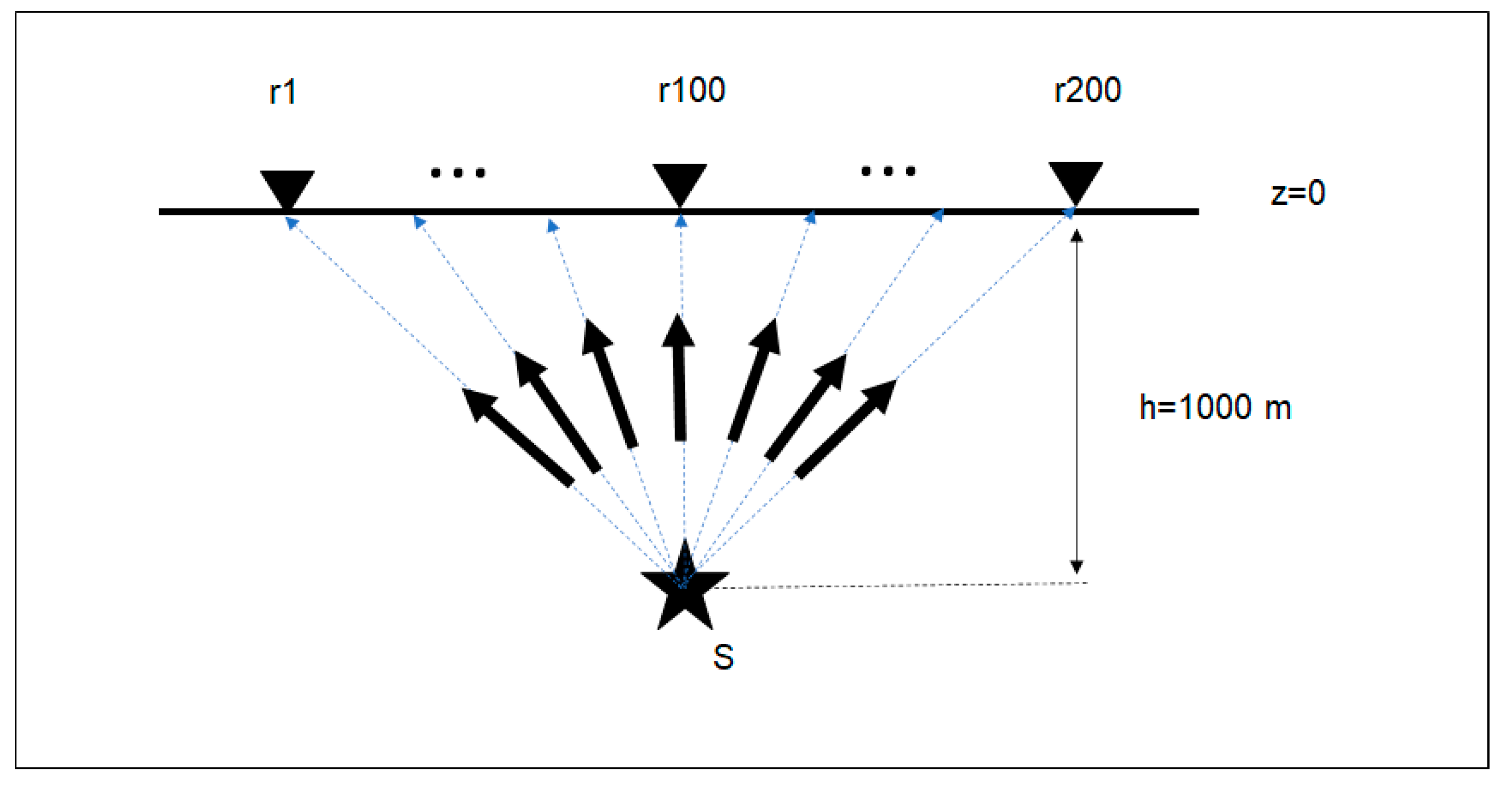
Consider the experiment shown in Figure 1, where a point source is located at S 1000 m depth. Two hundred receivers are evenly spaced at 25 m intervals along a horizontal surface at z = 0 on the surface. The source is located just below receiver station 100, and we use a Ricker wavelet with a peak frequency of 25 Hz. The model has a constant velocity of 2000 m/s. Three tests are performed, A, B and C, with a constant Q of 50, 100 and 200, respectively. For each test, we calculate the corresponding seismogram in the time domain, $u_{atten}\left(x_j,t\right)$—and $U_{atten}\left(x_j,\omega \right)$ is the seismogram in the frequency domain.

The seismogram of experiment A, with Q equal to 50 (Figure 2a), is flattened at 0.5 s, the apex of the hyperbola (Figure 2b). The amplitude spectrum of $U_{atten}\left(x_j,\omega \right)$ for Q equals 50 is shown in Figure 2c, where the frequency peak changes toward lower frequencies, away from the central trace $x_j$ = 100.

The summation of Equation (10) corresponds to the stacking of all 200 traces of $u_{atten}\left(x_j,t\right)$ in the time domain, with a radius of aperture equal to 2.5 km. The resulting trace $S_{atten}\left(x_j,\omega \right)$ has a peak frequency $f_p$ of 19.5 Hz for experiment A, with Q = 50. Using Equation (5) for t = 0.5 s, $f_m=25$ Hz, $f_p=19.5$ Hz, the effective Q for migrated data, $Q_{mig}$ is 39.

Additionally, in experiment A, if we assume a migration aperture equal to zero, we cannot use the stacked trace, but only the central one, $u_{atten}\left(x_j=100,\omega \right)$, for Figure 2b, whose peak frequency $f_p$ is 20.6 Hz. The calculation of the quality factor for a migration aperture of zero $Q_{mig}$ is equal to 50, the expected result.

The procedure described in the previous sections is repeated in experiments B and C, where the models have Q of 100 and 200, respectively. The results are shown in Figure 3, where the horizontal axis represents the effective quality factor of the migrated data ($Q_{mig}$) and the vertical axis represents the expected or actual effective Q. The orange squares and blue circles correspond to the migration apertures of zero and 2.5 km. For all experiments, the migrated data with zero aperture Q are equal to the expected one, $Q_{mig}$ = $Q_{eff}$. For a migration aperture of 2.5 km, the relationship between effective Q and $Q_{mig}$ is given by Equation (13).

$$Q_{eff}=1.3402 Q_{mig}-9.6892$$

(13)

The relationship between $Q_{eff}$ and $Q_{mig}$ derived above is based on a single diffraction curve for each experiment. However, in real data, there are multiple events that overlap. The migration process may use these unwanted overlapping signals to compose a particular diffraction pattern, which actually reduces the accuracy of the Q estimate. Despite this loss of accuracy, migration preserves the $Q_{eff}$ > $Q_{mig}$ characteristics and the relative and lateral contrast of high and low Q regions, providing semiquantitative subsurface information.

3. Application

The estimation of effective Q and its correction (Equation (13)) was performed on a migrated single-channel seismic dataset from the Joetsu Basin in the Japan Sea.

3.1. Joetsu Basin Geology and Characteristics

The Joetsu Basin is a known site of massive gas hydrates. Geological evolution and current tectonic activity favor the existence of upwelling gas plumes that cut through soft sediments and solid gas hydrate in the first hundred meters below the seafloor. The difference in the porous content of sediments results in unequal physical properties for the same lithotype. Heterogeneous velocity field and attenuation patterns are thus expected due to energy losses of the propagating wave front.

Gas Hydrate in the Joetsu Knoll, in the homonymous basin, lay along the first hundred meters of Neogene sediments that are mainly composed of clay and silt [23,24]. Upwelling gas locally cut the sediment pile through chimneys that reaches the seafloor and continues upward along the water column. Such a geologically active environment results in heterogeneous physical properties of sediments and rocks and their fillings (gas, water, or solid GH), which are sensitive to seismic signals.

Despite the available seismic data and geologic features, little research has been conducted on the Joetsu Basin to understand Q distribution and its relationship to gas hydrate and compression velocity (V_p). In reference [23], an average V_p between 1618 and 1659 m/s is reported for the Haizume Formation based on two wells drilled in Umitaka Spur, a structure south of the Joetsu anticline. The authors in reference [24] correlate the heat flow data, pressure–temperature curve of gas hydrate stability, and seismic two-way time of BSR and estimate the velocity of host sediments between 1000 m/s and 1150 m/s along the crest and between 1170 and 1230 m/s in the troughs. In paper [25], the authors use diffraction velocity analysis (DVA) to estimate a rms velocity between 1500 and 1580 m/s in the Haizume Formation.

3.2. Joetsu Knoll Shallow Sediments and Dynamics

The Joetsu Basin was formed 25 million years ago [26] as a segment of the Back-Arc system west of the Japan island arc. Its geologic and tectonic evolution can be found in [27,28,29] and are briefly summarized in [25]. Our analyses are conducted over the clay-rich sediments of the Haizume Formation, which have been deposited from the Late Pleistocene to the present.

The Joetsu Basin is a very active geological system, as folding of the very young Haizume Formation provides evidence of extremely active tectonics at the present time. In the paper [30], the authors report that the muddy seafloor of the Joetsu Basin currently has an average heat flow of 98 ± 13 mW/m², which exceeds 150 mW/m² at the methane venting and mounds along the Joetsu Knoll line. Reference [24] reports that mounds and pockmarks are 50 to 500 m wide and 10 to 50 m deep, which is related to gas chimneys below. The existing source rock of the Miocene units, the Nanatani and Teradomari Formations [28], the thermal history of the Joetsu Basin, and the vertical fault system at the apex of the Joetsu anticline provide conditions for the precipitation of hydrates in the Haizume Formation. According to [24], bottom simulating reflectors (BSRs) are often parallel to stratification and, based on gas hydrate stability conditions and heat flow information, BSRs are estimated to be 115 m below seafloor (bsf) at the crest of the Joetsu Knoll and 135 m in the trough.

3.3. Description of Geophysical Data

Seismic data were acquired in 2007 by the Japan Agency for Marine-Earth Science and Technology (JAMSTEC). The source, an air-gun cluster, was towed 30 m from the ship and depths ranged from 1.5 to 7.4 m; the receiver device was a streamer with 48 channels evenly spaced at 1 m intervals with a minimum offset of 136.5 m from the source. More details about the acquisition device can be found in [25].

After time shift correction, all recorded channels were stacked to create a single station per shot. The data were recorded at a sampling rate of 0.001 s. In this study, the five seismic lines used (Figure 4) are referred to as JKn, where n indicates the line number: 109, 114, 117, 124, and 153. JK153 is a strike line parallel to the Joetsu Knoll hinge and has a northeast direction. From southwest to northeast (Figure 4), observed dip lines JK109, JK114, JK117, and JK124 are orthogonal to JK153, and in a northwest direction. These lines are selected because of their extents and their long linear segments, which favor the processing flow and analysis.

In the following topics, sections with five attributes or properties are described: seismic amplitude, EHA, peak frequency, effective Q and V_p, showing the BSR and intersections with the crossing lines. The strike line JK153 always shows four vertical lines corresponding to the intersection with the dip lines JK109, JK114, JK117, and JK124. The dip lines are detailed in the discussion section and are shown with the interpreted BSR and with a vertical line representing the intersection with JK153. The JK-153 strike line is shown from left (SW) to right (NE), while the dip lines are all shown from left (SE) to right (NW).

3.4. Processing Flow and Property Estimation

The processing flow described in [25] was repeated individually for seismic lines JK109, JK114, JK117, JK124, and JK153. It included trace edition, static correction, bandpass filtering, predictive deconvolution, diffraction velocity analysis (DVA), Kirchhoff time migration, and muting above sea level. A trapezoidal filter with a frequency of 5–15–180–200 Hz was used in the filtering step. After applying the described processing procedure, the resulting strike section JK153 is shown in Figure 5.

3.5. Estimation of Velocity along Haizume Formation

The equivalent normal moveout velocity was estimated for each line using the DVA method described in [25]. The interval velocity V_p was estimated from the rms velocity [31] and used for imaging. The resulting V_p allowed the identification of the main trends, although it was too smooth and lacked the appropriate resolution to capture thin events and gas chimneys. Figure 6 shows the resulting interval velocity for the JK153 strike line in the time domain, indicating a general trend that increases from 1500 m/s at seafloor to 1750 m/s at 2.4 s. Smooth lateral velocity changes are observed along the section in the shallow region while, one of them, near station 2000, is close to a mound and the steeper slope of the Joetsu Knoll NE side (right side of Figure 6).

Each interval velocity section was time-to-depth converted. Then, we calculated the vertical gradient of V_p from the smooth velocity field in depth of Figure 6. The vertical velocity gradient provides information on how velocity increases with depth and is also a guide to the behavior of the compaction curve. A normal clastic sequence in a marine environment typically has vertical velocity gradients of about 0.600 s⁻¹ [32].

By counting the velocity gradients and distributing them at regular intervals, we constructed a histogram, which is shown in Figure 7. The highest value of the vertical axes (called density) shows the dominant trend of the velocity gradient in the horizontal axes, that is 0.225 s⁻¹ for the Haizume Formation. This value is much lower than the expected value of 0.600 s⁻¹ for a normal clastic compaction curve. The negative gradients present are mapped by DVA because they would be useful for mapping gas clouds, but higher resolution is required to use this information. Gradients of lower magnitude near to and higher than 0.600 s⁻¹ are also found in the dataset.

3.6. Enhancement of BSR

BSRs are generally not difficult to map. However, int the Joetsu Basin, however, they often occur parallel to stratification [23,24], making BSR mapping a difficult task. Under constant pressure, the bottom simulating reflector is an isothermal boundary that defines a phase transition (solid hydrate on top and gas on bottom) with high reflectivity that causes high amplitude in seismic records.

After normalizing the amplitudes, when powering the entire seismic data, using a value $p$ higher than 1, the contrast between high and low amplitudes, respectively ${u_{high}(x_{rec},t)}^p$ and ${u_{low}(x_{rec},t)}^p$, increases. If $p$ is a very high positive odd value, high-amplitude derived events (${u_{high}(x_{rec},t)}^p$) are preserved with their signal polarity, and (${u_{low}(x_{rec},t)}^p$) tends to zero. If $p$ is a very high positive even value, we obtain abs(${u_{high}(x_{rec},t)}^p$) and, again, (${u_{low}(x_{rec},t)}^p$) tends to zero. Thus, with suitable high $p$, the resulting section with enhanced high amplitudes (EHA) $u_{enhance}(x_{rec},t)$ is calculated as follows

$$u_{enhance}(x_{rec},t)={u(x_{rec},t)}^p$$

(14)

We power the processed seismic lines using $p$ equal to 10 (Equation (14)). This procedure enhances high-amplitude events and highlights the BSR along its expected position in the EHA lines. Figure 8 shows the EHA section for the JK153 strike line.

3.7. Q Estimation along Haizume Formation

The application of the windowed Fourier Transform, Equation (3), requires calibration of the σ parameter of the Gaussian function $g\left(t\right)$ to determine an appropriate time window size, since a low σ focuses the spectral response, while a high σ causes smearing with neighboring events. Since we performed trapezoidal filtering (5–15–180–200 Hz) in the processing flow, the data did not have a period above 0.2 s. We apply a σ that imposes a time window of 0.4 s, twice the maximum period, to allow proper evaluation of periods equal to or less than 0.2 s in the central region of the Gaussian curve, thus accounting for a low relevant frequency near 5 Hz. The existing smearing due to adjacent events is attenuated by the Gaussian tails.

From the amplitude spectrum of $U(x_{rec},\tau ,\omega )$, the peak frequency at each position and time is calculated using Equation (4). Figure 9 shows the spatial behavior of the peak frequency in section JK153. The attribute changes laterally, but it clearly shows the decreasing values from the seafloor to greater depths or higher times.

The effective Q ($Q_{eff}$) is calculated for each line using Equation (5). Equation (13) is used to compensate for the Q estimate because the aperture from which it is derived, 2.5 km, is the same size as that used for the migration of the Joetsu seismic lines.

Due to the lateral variations of the peak frequencies and their vertical gradients, the effective Q changes considerably. In the strike section JK153, Figure 10, a region with a mean $Q_{eff}$ of 50 is strongly confined to the occurrence of BSR. The NE limit of BSR, near station 2000, coincides with a remarkably low effective Q penetrating shallow sediments and also coincides with a known gas chimney, expressed by a mound on the seafloor (Figure 5 and Figure 9).The NE limit of BSR, near station 2000, coincides with a remarkably low effective Q penetrating shallow sediments, and also coincides with a known gas chimney, expressed by a mound on the seafloor (Figure 5 and Figure 9).

4. Discussion

We integrate the sections with enhanced high amplitude (EHA), peak frequency, effective Q, and velocity of each dip section, JK109, JK114, JK117, and JK124, as shown in Figure 11, Figure 12, Figure 13 and Figure 14, respectively.

The EHA sections, calculated by Equation (15), are very useful to map BSRs and confirm their existence, mainly along dip lines where this feature is harder to track. The EHA sections of lines JK109, JK114 and JK117 shown in Figure 11a, Figure 12a and Figure 13a, respectively, indicate a continuous BSR event that correlates perfectly with the strike section JK153 (Figure 5). The BSR is longer in JK109 than in JK114 and JK117. Comparison between the amplitude and EHA sections of the JK153 line in Figure 5 and Figure 8, respectively, shows that BSR mapping in the studied Joetsu area is facilitated by an enhanced high-amplitude attribute. In JK124, Figure 14, BSR is hardly observed with the EHA. Solid hydrate may disappear or become too sparse somewhere between lines JK117 and JK124.

The peak frequency values show a decreasing trend from the seafloor to higher times, or depths, along all seismic sections analyzed. However, the observed lateral changes impose vertical frequency gradient variation along each line. In the JK153 line, frequencies are higher than 120 Hz and reach 200 Hz near the seafloor (Figure 9). The gradient to low frequencies, below 90 Hz, are approximately higher along the region where the BSR is interpreted, indicating higher absorption in this region. Along lines JK109, JK114, and JK117, the higher gradient to lower peak frequencies is also consistent with the mapped BSR (Figure 11b, Figure 12b and Figure 13b) and coincides with the Joetsu anticline hinge. In section JK124, despite the absence of the mapped BSR, the higher gradient from high to low frequencies also occurs along the anticline hinge (Figure 14b), suggesting that this region is a site without massive hydrate, but with upward gas migration adjacent to a giant gas chimney, as also observed at station 2000 of the JK153 strike line.

A pattern change in the lateral distribution of peak frequencies is observed alongside the anticline structure. In JK109, frequencies are higher on the SE flank than on the NW flank (Figure 11b). All other dip sections, JK114, JK117, and JK124, show an opposite behavior, as the peak frequencies are lower in their SE flank than in the NW flank (Figure 12b, Figure 13b and Figure 14b). The reason for this behavior is not fully understood.

Effective Q values less than 100 and averaging 50 occur along a region larger than the BSR boundary, as observed in the JK153 strike line (Figure 10). These low $Q_{eff}$ values are found at the SE flank and the anticline hinge of JK109 (Figure 11c), while the average value of 50 is observed at the hinge and at both structure flanks on the JK114 (Figure 12c). The line pattern of JK117 is similar to that of JK109, but narrower than that of JK114 (Figure 13c). In addition, line JK124 shows the narrowest region with $Q_{eff}$ averaging 50 (Figure 14c). This northeastern narrowing and low $Q_{eff}$ value are consistent with northeastern narrowing of the anticline structure and the progressive decrease in hydrate concentration in the shallow region of the Haizume Formation. The Q factor is lower in hydrate-prone sediments than in sediments without hydrates [6]. The resulting geometry of low $Q_{eff}$ in the studied sections of the Joetsu anticline allows us to map the gas hydrate zone near the seafloor and the gas chimneys at depth.

In addition, hydrates do not occur as a continuous layer, but filling centimeter- to meter-thick pores and voids in the sediments of the Haizume Formation (Figure 15), due to the pressure and temperature near the surface, which are 9.0 MPa and 2 C, respectively. The contrast between the soft sediments and the distributed stiff solid hydrate results in scattering of the propagating wave field, which enhances attenuation and resembles apparent absorption. The combined effect of gas and seismic signal scattering by hydrate increases the attenuation, but it is not possible to distinguish the contribution of each one.

All analyzed lines have frequency peaks above 100 Hz, sometimes reaching 200 Hz, near the sea floor. Additionally, below a few seconds from the seafloor, all lines have frequencies close to 50 Hz. Therefore, seismic data with high-frequency content are needed for the proposed study, otherwise the absorption effect cannot be detected.

All estimated velocities show rather monotonous behavior, as can be seen in Figure 11d, Figure 12d, Figure 13d and Figure 14d. Despite their low spatial frequency, the DVA-derived interval velocity shows some upward gas chimneys directly beneath the mapped mounds. An example of this is at station 600 of line JK114 (Figure 12d), where the lateral velocity changes due to a gas chimney are also expressed by two mounds on the seafloor. DVA allows extraction of geologically possible features and provides normal move-out velocities for time migration. However, it lacks high-frequency information [12] for further estimation and interpretation. A detailed V_p field can be obtained with high-resolution tomography over multichannel seismic data, which were not accessed in this study. The most often vertical V_p gradient of 0.225 s⁻¹ is, indeed, too low for a shallow clastic sequence. The high heat flow [24,30,33], hydrocarbon (gas) generation, upward fluid migration, gas chimneys and local fluid entrapment increase the pore pressure, reduce the effective stress, and thus reduce the compression velocity and its vertical gradient.

5. Conclusions

In this study, we show that velocity gradient, peak frequency, effective Q, and EHA can be estimated from SCS datasets for subsurface geophysical characterization. In addition, we propose a linear correction for effective Q estimated from migrated datasets. Application of the techniques presented to the Joetsu Knoll SCS dataset leads to a number of new estimates and interpretations of Q and velocity at this site.

The DVA in the SCS does not allow estimation of detailed velocities, but provides a useful, smooth V_p field that can estimate the general trend. In the Haizume Formation along the Joetsu Knoll, velocities range from 1500 to 1750 m/s with a smooth trend of 0.225 s⁻¹, suggesting under-compaction of sediments.

The estimate of effective Q from migrated seismic data ($Q_{mig}$) preserves the relationship between areas of high and low Q. $Q_{mig}$ is always smaller than the effective Q estimated from non-migrated data ($Q_{eff}$). A linear correction with respect to the acquisition aperture (Equation (13)) can be applied to improve the $Q_{eff}$ estimate.

The area of low effective Q averages 50 and encloses gas hydrate. In addition to mapping the BSR and GH occurrence areas, it is also useful for locating gas chimneys. Gas hydrate geometry and width are due to anticline geometry, while northeastward narrowing is observed within the low-$Q_{eff}$ area. In this geologic context, sediment composition and granulometry, effective Q section or volume are important and useful seismically derived properties that can be used to automatically locate gas exudation and GH to support integration and interpretation tasks.

The gas hydrate and gas exudation region has a lower Q value than the sediment without free gas and GH. The tools presented in this research are useful for applications with similar datasets, SCS, in basins where there are hydrates and gas chimneys that affect seismic signals with strong absorption effects.