Abstract
The recycling or burial of carbon dioxide in depleted petroleum reservoirs and re-imagining exploration strategies that focus on hydrogen reservoirs (with any associated hydrocarbon gas as the upside potential) are a necessity in today’s environmental and geopolitical climate. Given that geologic hydrogen and hydrocarbon gases may occur in the same or different reservoirs, there will be gains in efficiency when searching for both resources together since they share some commonalities, but there is no geophysical workflow available yet for this purpose. Three-dimensional (3D) marine controlled-source electromagnetic (CSEM) and magnetotelluric (MT) methods provide valuable information on rock-and-fluid variations in the subsurface and can be used to investigate hydrogen and hydrocarbon reservoirs, source rocks, and the migration pathways of contrasting resistivity relative to the host rock. In this paper, a process-oriented CSEM-MT workflow is proposed for the efficient combined investigation of reservoir hydrocarbon and hydrogen within a play-based exploration and production framework that emphasizes carbon footprint reduction. It has the following challenging elements: finding the right basin (and block), selecting the right prospect, drilling the right well, and exploiting the opportunities for sustainability and CO2 recycling or burial in the appropriate reservoirs. Recent methodological developments that integrate 3D CSEM-MT imaging into the appropriate structural constraints to derive the geologically robust models necessary for resolving these challenges and their extension to reservoir monitoring are described. Instructive case studies are revisited, showing how 3D CSEM-MT models facilitate the interpretation of resistivity information in terms of the key elements of geological prospect evaluation (presence of source rocks, migration and charge, reservoir rock, and trap and seal) and understanding how deep geological processes control the distribution and charging of potential hydrocarbon, geothermal, and hydrogen reservoirs. In particular, evidence is provided that deep crustal resistivity imaging can map serpentinized ultramafic rocks (possible source rocks for hydrogen) in offshore northwest Borneo and can be combined with seismic reflection data to map vertical fluid migration pathways and their barrier (or seal), as exemplified by the subhorizontal detachment zones in Eocene shale in the Mexican Ridges fold belt of the southwest of the Gulf of Mexico, raising the possibility of using integrated geophysical methods to map hydrogen kitchens in different terrains. The methodological advancements and new combined investigative workflow provide a way for improved resource mapping and monitoring and, hence, a technology that could play a critical role in helping the world reach net-zero emissions by 2050.
1. Introduction: Challenges and Conceptual Models
1.1. Net-Zero Emissions and Geological Complexity Challenges
Easy-to-find oil and gas accumulations no longer exist, and the deepening climatic emergency is driving a global transition to low-carbon energy sources, such as native hydrogen and geothermal reservoirs. It is now widely believed that hydrogen could significantly abate CO2 emissions, and, hence, finding cheap clean sources of molecular hydrogen will play a central role in helping humanity reach net-zero emissions by 2050 and limit global warming to 1.5 degrees Celsius. Native hydrogen is cheaper to produce than current methods (i.e., green hydrogen from renewable or nuclear-powered electrolysis, grey/blue hydrogen from natural gas-powered steam-methane reforming, and brown/blue hydrogen from coal-powered gasification), with an estimated cost of less than USD 1 per kg. It is also attractive because of its sustainability since it is generated by geological processes, can be directly used in industrial applications, and does not require fossil fuels for production. Understanding the deep geological controls on the genesis and distribution of native hydrogen is, thus, of the utmost importance in our quest to exploit this vital natural resource and help reduce our carbon footprint. Moreover, geologic hydrogen and hydrocarbons may occur in the same or different reservoirs, and there will, therefore, be efficiency gains in searching for both resources together, unlike the conventional practice. Indeed, re-imagining exploration strategies to focus on hydrogen reservoirs with the associated hydrocarbons as the upside potential is called for in today’s environmental and geopolitical climate.
The focus of geophysical investigations into natural hydrogen and hydrocarbon gas reservoirs has now moved into frontier areas where structural complexity, heterogeneous overburden, and resource system fundamentals pose significant challenges [1]. The conventional hierarchical approach in hydrocarbon reservoir exploration (Figure 1a) and development (Figure 1b) have to be tailored to meet the challenges in this new environment. The main industry challenges in the exploration of commercial marine hydrocarbon and native hydrogen accumulations include the following: finding the right basin and play (requiring basin-scale investigations), selecting the right prospects (requiring prospect-scale investigations), and drilling the right well (requiring reservoir-scale investigations). These technical challenges derive mostly from geological complexity and, hence, require the robust integration of geophysical and geological data to reduce the exploration risk [1].
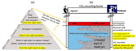
Figure 1.
Multi-scale challenges in reservoir exploratory and monitoring investigations with opportunities for carbon footprint reduction. The main objectives are highlighted in yellow, and the key technical challenges are in italics. (a) Conventional multi-scale hierarchical exploration approach. (b) Monitoring of hydrocarbon (or hydrogen) production and enhanced recovery aided by carbon dioxide recycling and/or chemical flooding of reservoirs. For completeness, the reservoirs should be investigated for permanent CO2 storage potential.
The seismic, controlled-source electromagnetic (CSEM), magnetotelluric (MT), gravity, and magnetic methods of geophysics play major roles in marine exploration for hydrocarbon and/or native hydrogen reservoirs. On their own, individual geophysical methods provide non-unique models of subsurface properties and the fluid type present, but integrating them [2,3] together with geological models maximizes accuracy, minimizes uncertainty in a “Shared Earth”, and leads to a consistent and possible indication of a working resource or surveillance system [1,4,5]. Optimizing this process has huge implications for time and cost savings, and there are opportunities for carbon footprint reductions at all spatial scales, as advocated for in this paper. It is also proposed here that any new hydrocarbon and hydrogen exploration plan must consider, as a top priority, whether such reservoirs can sequester CO2 for 100 years for net-zero emissions compliance (Figure 1). The traditional measurements in the search for hydrocarbons do not include hydrogen gas surveys, although hydrogen has been found to be associated with hydrocarbons in some wells. Perhaps now is the time to redress this imbalance in data collection. Along these lines, the appropriate conceptual models for electromagnetic investigations of natural hydrocarbon and hydrogen gas reservoirs are described in Section 1.2, and a new practical workflow is developed for the efficient combined investigation of these reservoirs in Section 1.3.
1.2. Conceptual Models for Electromagnetic Investigation of Hydrocarbon and Hydrogen Reservoirs
Important and, in some respects, unique information about a hydrocarbon gas-charged or hydrogen-filled reservoir can be obtained by measuring its electrical resistivity. Resistivity is a function of porosity, fluid saturation, temperature, and chemical composition, and hence the accurate 3D mapping and monitoring of this property in a reservoir is of practical importance and is remotely possible if the subsurface structural configuration is correctly specified using seismic, borehole, and other types of a priori information [2,6,7]. Figure 2 shows the relationship between bulk resistivity and resistive gas saturation ([8] Archie 1942) for different porosities (0.15%–0.3%), representing typical unconventional reservoirs (shales and tight sands) and porous clastic reservoirs (permeable sands and carbonates). It is obvious that the measurable bulk resistivity increases only marginally with low gas saturation but quite significantly with high gas saturation. This provides a justification for using electromagnetic methods for mapping and monitoring offshore hydrocarbon reservoirs [9,10].
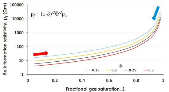
Figure 2.
A simple physical basis for mapping and monitoring bulk resistivity changes with fluid saturation in tight or porous reservoirs [8]. The relationship between the bulk resistivity of reservoir materials (ρf) and gas saturation (S) for four different porosities (Φ = 0.15, 0.2, 0.25 & 0.3) is shown, assuming a value of 0.33 for the fluid resistivity, ρw. The inset shows the equation used for calculating ρf [8]. For a given reservoir, the effect of injecting resistive fluids (e.g., CO2, natural hydrogen, and hydrocarbon gas) is to move up along the curve towards higher resistivity (as indicated by the red arrow), providing that the porosity does not change; if porosity is reduced due to new mineralization over time, we would expect one to move across the curves. In the case of brine or surfactant injection, it would move one down the curve rather than across the curves (depicted by the light blue arrow) unless the porosity changed in the process, for which one then moves across the curves.
The CSEM and MT methods are the principal resistivity-measuring tools for the remote investigation of hydrocarbon or native hydrogen reservoirs offshore, and three-dimensional (3D) surveying is the method of choice in frontier regions [1]. These methods probe from the near-seabed surface to several km in depth, making them ideal for investigating prospective sedimentary sequences above and below thick salt or igneous layers and any associated deep structural controls. Marine CSEM-MT 3D surveying requires setting up arrays of electric and magnetic sensors (or receivers) on the seafloor (Figure 3). A horizontal electric dipole (HED) source is towed about 20–50 m above the seafloor or 10–15 m below the sea surface when only CSEM measurements are required. The receivers (Rx) are laid out on a grid (Figure 3), typically staggered with the line and Rx spacing being ~1–3 km, depending on the target size and depth. The HED source is towed along each survey line starting in one direction (in-tow) from ~20–30 km away from one edge of the area of exploration interest to ~20–30 km beyond the other edge (out-tow) and transmitting signals of multiple frequencies (typically 0.1 to 10 Hz) whilst the boat is traveling at ~2 knots (3.704 km/h) [1]. The source may also be towed in between the lines of receivers (Figure 3). For studies of deep structural control or magmatic impact on the distribution of reservoirs, the receivers are typically left on the seafloor for 7 to 14 days in order to record sufficient MT periodicities and good quality data, depending on the water depth [11].
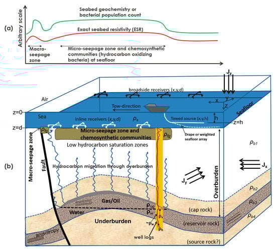
Figure 3.
A conceptual model and the marine CSEM-MT field set-up for mapping or monitoring a hydrocarbon-charged reservoir in heterogenous and anisotropic host sediments. (a) Cartoon showing the expected seabed profiles of electrical resistivity, geochemical anomalies, and bacterial population counts over a leaky hydrocarbon structural trap. (b) Cartoon showing a section through the leaky structural trap with seepage-related features near the seafloor and the typical 3D CSEM-MT survey layout [1]. Depth variations of background resistivity (ρb1, ρb2, ρb3, and ρb4) and anomalous 3D resistivities (ρog and ρfg) are indicated by the inset hypothetical well logs of the horizontal and vertical resistivities (ρh and ρv). Resistivity changes in the direction of the applied current for anisotropic materials, and Jx, Jy, and Jz are the associated current densities.
Electrical anisotropy is a major challenge in marine CSEM-MT exploration [1,12]. A conceptual model of a hydrocarbon-filled structural trap in the anisotropic ground is shown in (Figure 3). Localized 3D zones of chemosynthetic communities and patches of small-size bodies may abound in the near-surface, imparting strong heterogeneity, while at the reservoir level, anisotropy may be present in the form of laminations, microcracks, or other structural alignments. Inverting the complete, sufficient, and consistent marine CSEM-MT data to reveal the resistivity structure, taking into account 3D heterogeneity and anisotropy, is thus important for successful offshore reservoir mapping and monitoring. Industry benchmarking in 2017 revealed inconsistencies in horizontal and vertical resistivity distributions from anisotropic 3D CSEM inversion models produced by the major service providers for a given field dataset used for the test; invited academic practitioners abstained from the test [13]. This provided the motivation for the development of a crossgradient-based anisotropic-resistivity-imaging algorithm that directly enforces structural similarity between the horizontal and vertical resistivity models without control from seismic or well data [4,14,15]. The seismic, image-guided anisotropic 3D inversion of CSEM and MT data is an adaption of this crossgradient philosophy, in which the structural controls from seismic or other images are infused in the anisotropic resistivity inversion process [7,16,17,18].
The petroleum system model (source, reservoir, trap, and seal) is generally well-known. The presence and effectiveness of hydrocarbon source rocks, migration and charge, reservoir rock, and trap and seal (see Figure 3) are the critical geological attributes that must be satisfied for successful exploration and hydrocarbon discovery [19]. While 3D surveying is now well-established in marine CSEM-MT exploration in frontier regions, how to relate the information to the key elements of geological prospect evaluation (presence of source rocks, migration and charge, reservoir rock, and trap and seal) still remains a non-trivial technical challenge [1].
Surface seeps of native hydrogen are common in volcanoes, geothermal springs, and deep-rooted faults, but the native hydrogen system (source, reservoir, trap, and seal) is less well-known than the petroleum system model. The known favorable subsurface environments for the occurrence of native hydrogen include serpentinized ultramafic complexes in mid-ocean ridges, land-based ophiolite-peridotite intrusives (remnants of oceanic crust) (Figure 4a), and fossil arc-continent collision orogen (Figure 4b) [20,21,22]. The source rocks include ultramafic igneous rocks and iron-rich craton rocks [23,24]. The serpentinized mafic rocks at the base of the fossil subduction, obduction, and major thrust zones are known to produce fluids rich in native hydrogen [21,25]. Reservoir rocks include permeable, fractured basements and carbonate and marl or clayey rocks. They are often associated with ultrabasic or hyperalkaline waters (pH > 9) [26] and deep faults that tap basement or mantellic sources of hydrogen. The generation rate and preservation are unknown, and there is uncertainty about the size of the resource, but accidental discoveries suggest that subsurface accumulations are viable, such as those found on land in Mali, and the geological association with Precambrian crystalline shields was established [27,28,29].
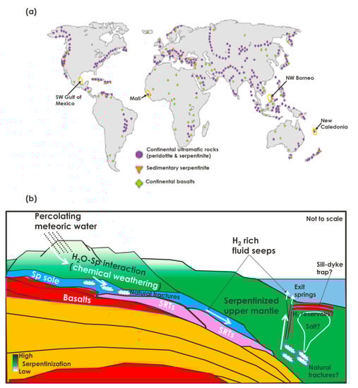
Figure 4.
(a) Global distribution of potential native hydrogen source rocks and reservoirs [20]. Main occurrences of peridotite and serpentinite on land are shown. Four locations discussed in the text (New Caledonia, Mali, NW Borneo, and SW Gulf of Mexico) are indicated by the orange ellipses and black arrows. (b) A conceptual model for the possible fluid-rock interactions in New Caledonia [21,22] and other similar hydrogen-rich ophiolite terranes; Sp: serpentinite; SRTs: subduction-related terranes. Sill-and-dyke trapping (akin to the situation in Mali) and diapiric salt reservoirs are only for illustrative purposes, but the salt structures have been identified elsewhere in the New Caledonia Basin [22]. Percolating meteoric waters interact with ultramafic mantle rocks to produce hydrogen-rich fluids. The natural fractures and faults provide pathways for the transport of the fluids and their eventual vertical migration into suitable reservoirs or exit springs on the surface. It is possible that there will be a meteoric fluid-serpentinite-evaporite hydrogen kitchen in this basin and similar geological settings around the world [22].
So far, it is known that methane and native hydrogen are produced in the competing processes of serpentinization and magmatism in slow- and ultraslow-spreading mid-ocean ridges, continental margins, and forearc settings of the subduction zones [21,30,31,32]. Serpentinization occurs when ultramafic rocks react chemically with invading seawater (or meteoric water) without biotic mediation, generating hydrogen, which can reduce carbon dioxide to methane. This is akin to the chemical weathering of the seafloor [24], and a similar process or an electrochemical mechanism may be operating on land to explain the discovery of native hydrogen in Mali [27]. This abiogenic chemical reaction leads to volume increases by up to 30% and the destruction of primary magmatic minerals [33] and, hence, new physical properties measurable by geophysical methods. Serpentinized mantle rocks are generally more conductive than mafic crustal rocks, such that electrical and electromagnetic methods can be used for their mapping, depending on their depth of occurrence. The hydrogen released during the serpentinization of ultrabasic rocks is one of the main fuels for chemosynthetic life [24], and the expected seafloor resistivity profile will be as in Figure 3.
The distribution of hydrogen and methane in the known reservoirs at the Bourakebougou field in Mali is shown in Figure 5. Hydrogen is lighter than methane, and its maximum concentration in these wells is found above that of methane. This fluid stratification based on density differences is similar to the arrangement in petroleum reservoirs. The Bourakebougou field consists of multiple layers of dolerite (diabase or micro-gabbro) sills serving as cap rock for multiple reservoirs, and the system is segmented by near-vertical fault-bounded dolerite dykes [27]. This mafic rock is chemically and mineralogically similar to basalt but is coarser-grained and contains silica; it may be no coincidence that basalt and gabbro form important layers of the crystalline crust in the known hydrogen-rich oceanic terranes [23]. The dominant reservoir at Bourakebougou is marble, but marl is an important reservoir (see Bougou-13 well in Figure 5). This reservoir specificity, the chemical weathering, evidenced by the thick lateritic cover in the area [27], and the fact that the total gas-rich column heights are identical for the wells, which are more than 4 km apart (red double-headed arrows in Figure 5), suggest the operation of a specific large-scale fluid-rock interaction process (perhaps involving meteoric alkaline waters and mafic rocks, with a possible contribution from along the steep faults tapping deeper sources). Electrical anisotropy will be expected across the prospective target depth here. Resolving the deep 3D electrical structure in such environments is important for understanding the geologic evolution of the hydrogen system [11].
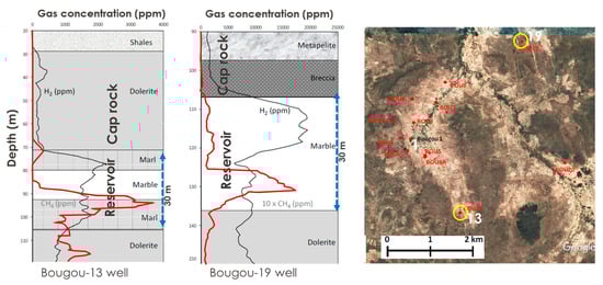
Figure 5.
Distribution of native hydrogen (H2) and methane (CH4) in two logged wells at the Bourakebougou field in Mali, modified from [28]. The variation of gas concentrations with depth in the host rocks is shown for hydrogen (black line) and methane (red line) for well Bougou-13 (left panel) and well Bougou-19 (middle panel). Although both wells are more than 4 km apart, the total gas-rich column heights (blue double-headed arrows) are identical. The right panel is a map showing the locations of the two wells, amongst others including Bougou-1, modified from [28].
1.3. Adaptive Play-Based Exploration Workflow for Combined Investigations of Hydrocarbon and Hydrogen Reservoirs
Although surface seeps and subsurface occurrences of native hydrogen are known, there is no framework for the geophysical exploration of reservoir hydrogen in potential hydrogen-rich geological settings. Geologic hydrogen and hydrocarbons may accumulate in the same or different reservoirs, and there will be efficiency gains in searching for both resources together, especially in offshore frontier regions. A template is provided in Figure 6 as a framework for the systematic investigation of hydrocarbon and/or native hydrogen reservoirs and their related structures in favorable geological settings. Here, the multi-scale three-step play-based exploration concept used for traditional petroleum exploration (Figure 1a) is appropriately adapted to the electromagnetic mapping and monitoring of hydrocarbon and native hydrogen reservoirs, with an emphasis on reducing carbon footprint. In this paper, it is stressed that the CSEM and MT methods can effectively contribute to optimizing all the phases of play-based exploration for hydrocarbon and/or native hydrogen reservoirs and their eventual monitoring (Figure 6), facilitated by new developments in data attribute analyses and three-dimensional (3D) anisotropic resistivity inversions of large-size survey data on high-performance computers. Since these methods provide valuable information on rock-and-fluid variations in the subsurface (Figure 2), they can also be used to monitor reservoirs, and a practical algorithm for 4D time-lapse resistivity imaging is proposed. It is also shown here that EM methods can contribute significantly to the understanding of deep geological controls on the distribution of hydrocarbon and native hydrogen reservoirs, leading to improved resource mapping and monitoring, hence a technology that could play a critical role in helping the world reach net-zero emissions by 2050.
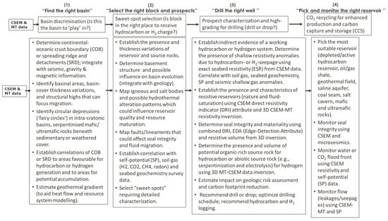
Figure 6.
A multi-scale process-oriented framework for combined investigations of hydrocarbon and hydrogen reservoirs using CSEM-MT methods. It extends the conventional three-phase play-based exploration approach (Figure 1a) to allow for reservoir development and monitoring that are beneficial to carbon footprint reductions.
2. Quantitative Methodological Developments
2.1. Geologically Consistent CSEM Multi-Attribute Analysis: Effective Prior Settings for Optimized 3D Inversion
A recent practical development in marine CSEM data processing is the multi-attribute analyses of field data that enable a simple, rapid assessment of the key elements of geological prospect evaluation: the presence of source rocks, migration and charge, reservoir rock, and trap and seal [1] and is particularly relevant for the optimized mapping of stratigraphic traps. A simple geometrical normalization of CSEM amplitude data yields what is termed a direct resistivity indicator (DRI) attribute and can facilitate the retrieval of the exact seafloor resistivity (ESR) and layered background resistivities in ideal conditions [1]. The DRI attribute is also used to obtain edge-detection attributes (EDA) for finding the horizontal position and shape of anomalous 3D bodies [1]. While CSEM is a proxy method for reservoir detection, unlike the more direct seabed geochemistry and seismic methods, combining DRI, ESR, and EDA can help improve objectivity or modify decision-making based on the conventional subjective geological risk evaluation of petroleum ventures [19].
The main benefits for geological venture risk evaluation can be summarized as
- DRI attribute shows the existence of a regional resistive play or carrier bed (characterized by symmetric in-tow and out-tow response profiles) and the desirable localized 3D resistors (characterized by asymmetric in-tow and out-tow response profiles). This meets the geological requirement for identifying the presence of reservoirs (regional plays or localized traps of exploration interest) in frontier regions. This attribute facilitates the rapid screening of CSEM data to select areas warranting follow-up, expensive, and rigorous 3D inversion, leading to significant efficiency gains and computational cost savings [1]. It is best used for the rapid polarization (ranking) of a portfolio of leads and prospects in offshore regions where there are competing targets previously identified using seismic data [1,34,35];
- The effective area or size of a hydrocarbon-charged 3D reservoir is a key requirement in reserve estimation [19]. EDA permits the accurate determination of the exact lateral boundaries of 3D resistive targets and, hence, the effective area necessary for reserve estimation;
- The ESR attribute provides a link to geochemical seabed data, and together these permit a judgment regarding the presence of a working petroleum system (i.e., presence of charge). The ESR profiles sample the near-surface area (top 10–50 m of the seabed based on skin-depth considerations) and should ideally correlate with seabed geochemistry profiles or seismic shallow gas clouds and, thus, provide a basis for comparing or integrating these disparate datasets to confirm the presence of a working petroleum system [1];
- The results from the analyses of these attributes make up the initial model m0 (i.e., robust model priors) for the subsequent tailored 3D-depth imaging of targeted reservoirs [1].
2.2. Geologically Consistent 3D Anisotropic Resistivity Inversion: Robust Depth Conversion
It is emerging that integrating 3D anisotropic CSEM-MT data imaging into seismic or structural constraints leads to geologically robust models [4,7,15]. Two methods of geologically consistent 3D anisotropic CSEM and MT resistivity inversion (using crossgradient constraints) have recently been developed [7,15,18] and are briefly described below.
In the first method, the MT and CSEM data are inverted for the vertical and horizontal resistivities directly while imposing a crossgradient constraint to ensure the structural similarity between the models [14,15]. The objective function to minimize can be stated as
where d represents the observed MT and/or CSEM amplitude and phase data, f(mv,h) are the model responses predicted by 3D anisotropic forward theory, is a weighting matrix whose entries are the inverse variance or covariance of , and mv and mh are the sought vertical and horizontal resistivity models, respectively. R is the Tikhonov regularization operator, and the pre-multipliers α and β are weights selected by initial trial-and-error testing [17,36]. The third term on the right-hand side is the non-linear crossgradients operator, or structure-promoting regularization [37], where and are the gradients of the vertical and horizontal resistivity models, respectively. The fourth term on the right-hand side contains the statistically independent a priori information mv,h(ref), such as from seismic or well log data that are wished to be retained in the solution, and contains the variances of the sought anisotropic model parameters. More details of this inversion approach are given elsewhere [15].
In the second method, the CSEM and MT data are jointly inverted using the nonlinear crossgradients operator to relate the horizontal and vertical resistivities as before, but they additionally imprint structural fabric from 3D seismic reflection images onto the resulting models using a linear crossgradients operator [7]. This is equivalent to the use of statistically independent a priori information to constrain the resistivity inversion process. The resistivity models are guided by structure tensors computed from good quality 3D pre-stack depth migrated (PSDM) seismic data instead of using interpreted seismic horizons that might be subject to the interpreter’s error. The composite objective function to minimize can be stated as
where the gradient field derived from seismic structure tensors is fed into the last term on the right-hand side and represents a linear operation since these seismic gradients are fixed as statistically independent from the a priori information. The other terms have the same meaning as in Equation (1). The pre-multipliers α, β, and τ are also selected by initial trial-and-error testing. More details of this 3D seismic image-guided inversion method can be found in [7]. Equations (1) and (2) are solved in the adopted inversion program RLM3D using a nonlinear conjugate gradients algorithm [38] that is well-suited for this type of large-scale optimization problem.
2.3. Electrostratigraphic Imaging: Accurate Post-Inversion Reservoir Boundary Mapping
It is also emerging that the gradient information in 3D resistivity images can be used to relate the structure of the objects in the mv and mh models that are derived from the above anisotropic inversion methods or simply for identifying features of interest (e.g., edge detection) for direct boundary recognition [11]. For simplicity, one can exploit the magnitude of the directional derivative of either mh or mv implemented by differing between the neighboring pixels in the 3D model. The sought maximum change in pixel values for boundary detection in smoothness-constrained 3D resistivity models is defined as [11]
where the partial derivatives Ix = and Iy = are the pixel-based estimates of the components of the gradient vector computed using the forward or central differences between neighboring pixels in the given 3D subsurface resistivity model. The output of Equation (3) is termed the “total gradient” in order to distinguish it from the first vertical derivative (“1VD”) at a point, which was also shown to be equally useful for boundary detection [11].
2.4. Structurally Consistent 4D Time-Lapse Electromagnetic Imaging: Robust Fluid Tracking
Equations (1) and (2) can be adapted to any multi-set electromagnetic data and, hence, can be used to estimate the changes Δm1 due to dynamic processes in the subsurface monitored using the baseline data (d0) and monitor data (d1) acquired at different times: t0 and t1 [39]. Here, the reference anisotropic resistivity models are the models (mbase (v,h)) from the crossgradient inversions of the baseline 3D survey data (d0). In the case analogous to Equation (1), for any given base and monitor surveys, the basic problem statement is posed as minimize:
where the various parameters are as previously defined. Note that the last term on the right-hand side of Equation (4) can be replaced by the measure as the equivalent implementation of image-guided inversion (see Equation (2)). Equation (4) is solved using a nonlinear conjugate gradients algorithm [38] for this large-scale optimization problem.
In the geologically complex areas where the search for new energy-fluid reservoirs is taking place, it is critical to integrate various geophysical, geological, and environmental modeling tools in three dimensions so as to increase accuracy and, hence, reduce uncertainty in the conventional 3D subsurface predictions [2,40]. The integrated tools can also be used to monitor reservoirs during CO2 recycling and/or sequestration (Figure 1b), which are important for meeting the global net-zero emissions target. Improving the methodologies for geologically consistent multi-physics time-lapse imaging and uncertainty quantification [2,39,41,42] should, therefore, be seen as the way forward. For the n-type (multi-modality) geophysical measurements, we can apply crossgradient joint inversion to assure structural consistency between the respective model parameter changes Δm derived from the multi-modality baseline and monitor datasets. For notational simplicity, let us denote our anisotropic models for the multi-modality geophysical systems at the base survey time t0 as and those at the monitor survey time t1 as . The joint multi-physics inversion problem is then posed as minimize [2,39]:
subject to the condition
where , and the desired model changes are Equation (6) holds for all the possible crossgradient combinations equal to zero, as long as the selected g-pivot image is set to . This constraint will impose a resemblance between the multiple geophysical images as long as the g-pivot image has no null gradient [2]. The geophysical method with the highest subsurface resolution capability may be selected as the g-pivot set (e.g., seismic reflection, if this is available for this quantitative integration), but the pivot image can be varied for each position in the 3D model if the use of the morphology of a single-image property is not intended. Equations (5) and (6) can be solved using a nonlinear conjugate gradients algorithm [38]. Overall, the benefits of such a combined approach can be summarized as
- Risk mitigation in frontier ventures with no wells or good quality seismic data;
- Reduces the need to drill unnecessary wells, leading to significant cost savings;
- Potential to reduce prospect evaluation/maturation period;
- Maximize accuracy and reduce uncertainty, especially with regard to reservoir properties;
- Applying such a quantitatively integrated methodology can contribute significantly to a better understanding of the geological controls of the transport and distribution of fluids in clean-energy (especially geothermal and hydrogen) reservoirs, leading to improved resource mapping and monitoring, and hence, a technology that could play a critical role in helping the world meet the net-zero emissions target.
3. Instructive, Process-Oriented Case Studies
The recent results of 3D inversions of CSEM and MT survey data from large-scale industrial surveys in deep waters in NW Borneo [43] and the southwestern Gulf of Mexico [11] are revisited and interpreted here in the context of the proposed extended play-based framework for finding and monitoring hydrocarbon and hydrogen reservoirs (Figure 6), and the new lessons learned are discussed.
3.1. Play-Based Exploration in Deep Water in NW Borneo
3.1.1. Find the Right Basin and Play
A good place to select a new exploration block will be in a basin with proven plays, or that is near an existing field. The area of study is located in the fold-and-thrust belt of offshore northwest Borneo in water depths ranging from about 500 to 1600 m in the South China Sea (Figure 7a). It is known to be structurally complex, and the sedimentary rocks are mostly stacks of thin, bedded sand in shale, characterized by low resistivity and low contrasts [15]. The Miocene-Pliocene stratigraphy and the main turbidite fan intervals in this region [44] are shown in Figure 7b. At least seven turbidite fans have been identified as the reservoir targets. These were deposited in basin floor systems [44]. The structural style here is characterized by northeast-southwest trending ridges that are formed by elongated thrust anticlines, with intervening mini basins and toe thrust zones [15,17,44]. The hanging wall anticline with four-way dip closure is the main sought-after trap style in this area, while the stratigraphic plays located in the syncline remain under-explored.
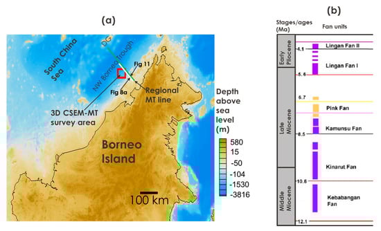
Figure 7.
(a) Map showing the location of the 3D CSEM-MT survey area in offshore NW Borneo. The thick white line is a 120 km-long regional MT survey line, for which the result is summarized in Figure 8a. The thick green line is the location of the model shown later. DG: Dangerous Grounds. (b) Mio-Pliocene stratigraphy and the main turbidite fan intervals in the study area [44].
The results from the recent use of regional MT inversion for basin-scale play mapping in this petroliferous deep-water fold-and-thrust belt are shown in Figure 8a. The objectives were to understand the basement structure and the distribution of potential hydrocarbon plays in the basin [43]. The full tensor data for the MT line were inverted in 3D, taking into account seafloor topography and electrical anisotropy. The inversion was unsupervised (i.e., initiated with half-space featureless starting anisotropic models) to also test the MT data resolution capability. The interpreted acoustic basement and the crust-mantle interface (Moho) from the CRUST1.0 seismic compilation [45] are plotted on the MT image of Figure 8a for comparison. The MT imaging detects a resistive basement (RB in Figure 8a), for which the top varies in depth from 10 to 15 km, and defines a mini foreland basin beneath the exploration blocks of interest. The basement cover rocks contain a resistive play (RP in Figure 8a) that is overlain by a conductive layer (possible cap rocks) and underlain by a thick, conductive layer (possible source rocks and detachment zone). Note the interpreted subhorizontal detachment zone into which root the steep-thrust faults demarcating sedimentary wedges or segments. Notice the apparent discrepancies between the regional MT result and the predicted acoustic basement and Moho in Figure 8a, especially the foreland mini-basin (flexural moat?) and major subhorizontal detachment suggested by MT imaging in the region, where seismic data are of poor quality.
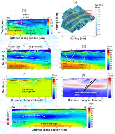
Figure 8.
Concept of ‘finding the right play’ and ‘selecting the right blocks and prospects’ is demonstrated using anisotropic resistivity models from 3D MT and CSEM inversion [43]. (a) Horizontal resistivity cross-section extracted along the white line in Figure 7a from a 3D model generated by an anisotropic inversion of regional MT data. The actual MT field data and the model verification using resistivity logs from several exploration wells are presented in [7,17]. RP is a resistive play (clastics). The independently interpreted acoustic basement (AB) and the crust-mantle interface (Moho) from the CRUST1.0 seismic compilation [45] are shown only for comparison. (b) Seismic depth map of the top of the Kebabangan reservoir, showing the structural pattern. Yellow dots are CSEM-MT stations [17]. Yellow lines are the dip line and strike line, along which were extracted the sections from joint CSEM-MT inversion, as shown in (c–g). The red boxes (1, 2, and 3) are potential sweet spots selected for detailed investigation. (c) Dip-section extracted from the 3D horizontal resistivity volume resulting from joint CSEM-MT inversion. (d) Our structural interpretation of the image shown in (c), together with independently interpreted seismic horizons (thin black lines) clearly demonstrates the geological consistency between CSEM-MT and the seismic results. The thick black lines show the interpreted subhorizontal detachment zone and steep-thrust faults demarcating sedimentary wedges or segments. (e) Vertical resistivity section and (f) anisotropy section extracted along the dip line from the anisotropic joint CSEM-MT inversion models. (g) Strike section extracted from the 3D horizontal resistivity volume, resulting from joint CSEM-MT inversion.
3.1.2. Select the Right Block and Prospects
An example result of large-scale 3D CSEM-MT surveying for multi-block mapping and evaluation in this basin is presented in Figure 8b–e. An important objective was to better understand the effect of basement control on the surface deformation and hydrocarbon distribution in the blocks. Two vintage MT-CSEM surveys were acquired for the client and were processed by EMGS in 2015 and 2016 over the area of the study [7,17]. The combined number of receivers from both surveys was 647, with a receiver spacing of 1.5 to 2 km in the 2015 prospect-specific localized acquisitions and 3 km for the large-scale regional acquisition in 2016 [7,17]. The 2016 3D EM survey has the largest 3D grid coverage of EM data ever recorded in a single survey in Malaysia and was used to generate the results presented here (Figure 8b). There are four wells (A, B, C, and D in Figure 9a) in the area, and these provided resistivity logging data for verification of the CSEM-MT result. The electric field CSEM data for five frequencies (0.125, 0.375, 0.625, 2, and 2.125 Hz) at source-receiver offsets ranging from 1000 to 10,000 m, and the full bandwidth of the recorded MT frequencies (0.000667 to 1.443 Hz) were utilized in the 3D inversion aimed at rapid regional prospectivity scanning. The model grid size was 312 × 199 × 145 cells in x, y, and z directions (excluding air layers) with cell sizes of 250 × 250 × 25 m with incorporated bathymetry. The cell sizes in the z direction increased by some factors as the deepest bathymetry was reached. The seawater resistivity values were derived from a sound velocity profile measured by EMGS during data acquisition and were kept fixed during the inversion. This dataset was used in testing the seismic image-guided joint CSEM-MT inversion [7], but the focus was not on petroleum system evaluation or understanding the influence of the deep basement on the gravity-driven deformation of the play, as attempted here. A structurally guided 3D inversion of all the MT data is reported elsewhere, but the focus here was on determining the best structural control to use via a comparison with the well log data [17]. These previous studies show the quality of the data and how well they are matched by the 3D model responses, and it will serve no further purpose to reproduce them here. What is new here is the play-based geological analyses of the joint inversion results in terms of petroleum and hydrogen systems and net-zero emission considerations. The results presented here are important for optimized resource system evaluations because
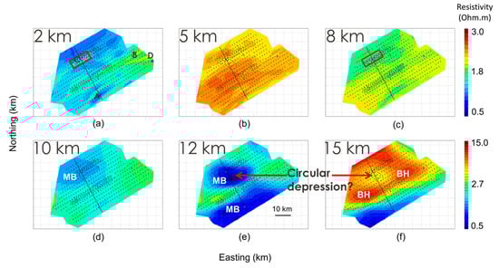
Figure 9.
Concept of selecting the right prospect to drill in the right mini basin or structural compartment. Shown are the horizontal slices at six different depths (2, 5, 8, 10, 12, and 15 km) in the 3D resistivity model derived from the seismic structure-constrained inversion of MT data [17] to show basin evolution in space and time and facilitate the selection of the best sweet spot for drilling. MB: mini basin; BH: basement high. A, B, C and D are the locations of drilled hydrocarbon exploration wells. The black dots are marine MT stations. The red rectangle was picked as the sweet spot with the best potential for finding a hydrocarbon-charged reservoir.
- The main plays in the blocks were clearly mapped based on their resistivity and anisotropy characteristics, as illustrated in Figure 8c,e–g. The 1–3 km thick conductive overburden (potential cap rock), resistive units (potential reservoirs in the turbidite fans), thick conductive underburden (possible source rock and shale detachment zone, as shown in Figure 8f) forming the post-rift play and rifted resistive basement with possible syn-rift play are evident;
- Structural compartmentalization is present in both the dip and strike directions (Figure 8c,e,g), which suggests the presence of different thrust wedges that are possibly separated by transfer faults, allowing relative block motions, with each compartment associated with a different prospectivity;
- The relatively rugged seabed topography suggests a recent deformational event and is structurally related to the geometry of the detachment zones in the upper 5 km in the resistivity anisotropy model (Figure 8f). The consistency between seafloor deformation and subsurface resistivity anisotropy suggests the active deformation of the sedimentary pile above the basement [11];
- The structure with the highest seabed expression is underlain by a steep southerly dipping basement edge, forming a buttress against which the transported sediments appear to have deformed considerably; this suggests a significant risk to any hydrocarbon accumulation; hence, the preferred sweet spot is the less disturbed fold structure properly centered on the basement high, which will focus hydrocarbon migration;
- The resistivity model is geologically consistent with seismic structure (Figure 8d), assuring confidence in the above interpretations and allowing the selection of the prospective play segments, dubbed “sweet spots” (Figure 8c,e), warranting further detailed integrated geological and geophysical analysis.
3.1.3. Drill the Right Well
Detailed examination of the time-space variation in resistivity provides further insights on basin evolution to aid the selection of the right block segment or ‘sweet spot’ to drill, as demonstrated in Figure 9. The key messages from this figure are the following:
- The horizontal or seismic horizon-controlled resistivity slices, extracted at different depths from the 3D horizontal resistivity model, revealed how the basement structure influenced basin evolution (the vertical resistivity model could also be used for this);
- The presence of a circular depression beneath the sedimentary cover. A localized circular mini basin can be seen in the 15, 12, and 10 km depth slices (possibly a mini foreland basin due to flexural response to loading and/or igneous intrusion). This is overlain by a clastic play comprised of resistive (sandy or carbonate-bearing reservoir rocks) and conductive (shaley source and/or cap rocks) materials, as revealed by the horizontal resistivity slices at 8, 5, and 2 km depths. Pockmarks were observed on the seabed in this locality. Well C (Figure 9a) was drilled in 2016 and encountered hydrocarbons at the predicted reservoir. Unfortunately, the measurement of hydrogen gas was not considered at the time;
- Could this circular basin be a hydrogen prospect? The observed pockmarks suggest the presence of chemosynthetic communities, analogous to what is observed across ‘fairy circles’ on land, characterized by seepages of native hydrogen. It will be interesting to survey this area for native reservoir hydrogen in a future effort to help reduce the carbon footprint. A seafloor 3D self-potential survey and geochemical soil gas sampling for H2, CO2, CH4, and radon, followed by the appropriate gas sampling in the wells, will be the recommended way forward here.
3.1.4. Pick and Monitor the Right Reservoir
An important consideration in any future investigations in this area will be the possibility of re-using the hydrocarbon reservoirs or saline aquifers for carbon sequestration. Figure 10 shows the result of the crossgradient 3D CSEM inversion for structurally consistent vertical and horizontal resistivity distributions for one of the three selected sweet spots (sweet-spot 3 in Figure 8b) [4]. The key messages from this figure are the following:
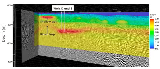
Figure 10.
Step 3: Drilling the right well, as demonstrated for sweet-spot 3 [4]. Shown here is the result of prospect-scale 3D CSEM resistivity inversion integrated with the seismic PSDM data for improved decision-making [4]. Note the blown trap beneath the shallow gas accumulation. Parts of this reservoir may, therefore, not be selected for future CO2 storage.
- Two wells sampled hydrocarbon at a depth correctly predicted by the 3D CSEM inversion (Wells D and E in Figure 10). So, this technology is useful for detecting and mapping potential hydrocarbon-charged reservoirs in this geologic setting;
- Note the strong presence of shallow resistive gas (evidence of a working petroleum system). A future 3D SP survey will be useful for assessing the gas flow pattern here;
- There is no major resistive cover at the crest of the anticlinal structure below this resistive shallow gas zone. This suggests that it is likely a blown trap allowing hydrocarbons to migrate vertically upward to form the observed shallow gas body. Parts of this reservoir may, therefore, be sub-optimal for future CO2 storage.
3.2. Understanding Deep Geologic Controls on the Genesis and Distribution of Hydrogen in the Investigated Area
It is widely believed that there is a fossil subduction system in the region of the MT surveys in offshore Borneo (Figure 7a). It was proposed that during the Paleogene, the Proto-South China Sea was subducted beneath northern Borneo and that subduction ended with the collision of the Dangerous Grounds block (Figure 7a) and the Sabah–Cagayan Arc in the Early Miocene [46]. Figure 11 shows the result of the 3D MT inversion of a regional survey line crossing the NW Borneo Trough (see the green line of the section in Figure 7a). Notice the conductive zone above the resistive mantle in the northern half of the profile. This is possibly serpentinized mantle. There are also possible deep-rooted faults extending from below the seismically inferred Moho. These could allow for the tapping of mantellic sources of hydrogen. At the top basement level, there is a major detachment zone. These are the features expected in a favorable terrane for the genesis and migration of natural hydrogen see [21,22,23,24,25]. So, the same electromagnetic dataset acquired for hydrocarbon exploration can be used for an extended search for potential natural hydrogen targets. The implications from Figure 11 are the following:
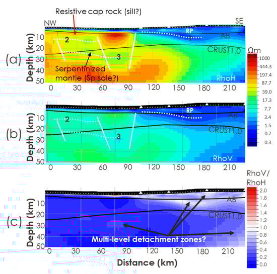
Figure 11.
MT resistivity and anisotropy sections across a proposed fossil subduction zone in offshore NW Borneo. The transect is shown in Figure 7a. (a) Horizontal resistivity. (b) Vertical resistivity. (c) Resistivity anisotropy. The thick white lines in Figure 8a,b are potential deep-rooted faults that can aid fluid migration; RP is the same regional clastic play shown in Figure 8, and the dashed white lines, 1, 2, and 3, are conductors and are possibly thrust-related since they have relatively high anisotropy (Figure 8c). The black interfaces are the interpreted regional acoustic basement from pre-stack depth-migrated seismic data (AB) and the CRUST1.0 Moho [45]. Sp: serpentinite.
- MT imaging can detect anomalous, electrically conductive basement rocks. There are two interesting conductive bands (see the dotted white lines 1 and 2 in Figure 11) in the western half and a shallow conductive detachment in the eastern half of the transect. The deeper conductive band may be thrust-related and associated with serpentinized mantle rocks, which are important sources of native hydrogen. Note the possible structural similarity with the serpentinite sole in Figure 4b;
- MT imaging can robustly map deep-rooted steep faults (thick solid white lines in Figure 11) that may be tapping deep mantellic sources and act as a migration pathway to potential reservoirs at higher levels;
- There appear to be suitable cap rocks for hydrogen accumulation, such as electrically resistive igneous rocks (sills?) and conductive claystone or detachment zones, as suggested in Figure 11. Clays and igneous rocks are known to form cap rocks for significant hydrogen reservoirs elsewhere (e.g., Figure 5);
- The zones of relatively high anisotropy in the crust and mantle shown in Figure 11c may be multi-level detachment zones, suggesting active deformation involving a combination of tectonic- and gravity-driven processes.
4. Discussion
4.1. Extended Play-Based Workflow for Combined Hydrocarbon and Hydrogen Investigations
An important thrust of this paper is the demonstration that a given large-size marine electromagnetic survey dataset can efficiently contribute to the understanding of deep geological controls on the genesis and distribution of both hydrocarbon and native hydrogen targets, leading to improved efficiencies in resource mapping and monitoring, and represents a technology that could play a critical role in meeting the net-zero emissions target. A framework is provided in this paper for the systematic combined investigation of hydrocarbon and hydrogen reservoirs and how their genesis and distribution are influenced by deep subsurface processes in favorable geological settings (Figure 6). The well-known concept of a ‘petroleum kitchen’ and the emerging hypotheses on the ‘hydrogen kitchen’ are integrated with a play-based exploration concept (Figure 1a) to yield a practical framework for the electromagnetic mapping and monitoring of hydrocarbon and native hydrogen reservoirs with implications for carbon footprint reduction (Figure 6). It is stressed that electromagnetic methods can effectively contribute to optimizing all the phases of play-based exploration for these reservoirs and their eventual monitoring facilitated by new developments in CSEM multi-attributes analyses and the 3D anisotropic resistivity inversion of large-size CSEM-MT survey data on high-performance computers. The case studies presented in this paper specifically show how marine CSEM and MT data imaging facilitates decision-making in the industry from the basin scale through to the prospect scale and the reservoir scale. The past works in this basin [7,17,43] focused on deriving resistivity structures that were structurally consistent in a hydrocarbon exploration context and considered neither the full geological implications for resource mapping and monitoring nor the possibility for natural hydrogen exploration and carbon footprint reduction. Unlike the common practice, this paper also demonstrates the interpretation of 3D resistivity information in terms of the key elements of geological prospect evaluation (presence of source rocks, migration and charge, reservoir rock, and trap and seal) and the use of electromagnetic models to understand the influence of geological processes on the genesis and distribution of potential hydrocarbon and native hydrogen reservoirs. This is a somewhat radical CSEM and MT approach but has been tested in several geological terrains using expensive industry-type data and is particularly relevant as the deepening climatic emergency now drives a global transition to low-carbon energy sources.
4.2. Wider Implications for Mapping Low-Carbon Reservoirs, Source Rocks, and Migration Paths
Understanding the deep crustal structure of geologically favorable environments for the genesis and accumulation of natural hydrogen should be considered a necessity in any practical exploration campaign since hydrogen is considered to be a key commodity in the low-carbon energy transition. Abundant geologic evidence shows that mafic and ultramafic rocks at the base of fossil subduction-obduction and major thrust zones, serpentinized ultramafic complexes in mid-ocean ridges, land-based remnants of oceanic crust (Figure 4a), and fossil arc-continent collision orogen (Figure 4b) produce geological fluids rich in native hydrogen [21,24,25]. It is known that surface seeps of native hydrogen are common in volcanoes and geothermal springs. It is also accepted that the source rocks for native hydrogen include ultramafic igneous rocks and iron-rich craton rocks [23,24]. However, the lithospheric structure across such terrains is often not well understood due to a lack of 3D pre-stack depth-migrated (PSDM) seismic data that have been the mainstay of the oil and gas industry [11]. It has been demonstrated (in Figure 11) that the deep marine MT imaging of fossil subduction or thrust zones is feasible using legacy MT data acquired for hydrocarbon exploration. Evidence of deep-rooted (extensional?) faults, possible serpentinized mantle, and resistive caps below the sedimentary cover are apparent in Figure 11. It will be instructive to examine whether the same can be achieved for fossil mid-ocean ridges, where serpentinization and magmatism are competing processes for the generation of hydrogen-rich fluids.
The results from a recent 3D marine MT investigation on the Mexican Ridges fold belt in the southwest of the Gulf of Mexico are re-analyzed here in Figure 12, Figure 13 and Figure 14. The area of study lies at the apex of the extinct Jurassic seafloor spreading center in the Gulf of Mexico [47,48] (Figure 12a). A banded crystalline basement structure was found across the fossil-spreading center comprising WSW-ENE trending, 6–10 km wide, electrically resistive subvertical sheets with conductive and anisotropic borders (Figure 12b), which merge into a basal resistive stock-like body at a depth of 15–20 km. NNW trending major faults were also found to cut the steep banded system. The resulting MT-evinced WSW and NNW structural trends, if rotated clockwise by 25–30 degrees, correlate with the previously interpreted transform and normal faults that formed during the Late Jurassic opening of the Gulf of Mexico [11]. The conductive bands spatially coincide with possibly fluid-filled vertical fracture sets in the overlying sediments, as seen in the seismic data (Figure 13 and Figure 14), and were, therefore, interpreted as hydrothermal fluid pathways [11]. In terms of trapping mechanisms, it is interesting that an electrically conductive subhorizontal detachment zone in Eocene shale deposits at a depth of about 5–6 km was found to act as an effective barrier to vertical fluid migration (Figure 13 and Figure 14). There are also microseismic activities in the area, and Meju et al. [11] inferred that a magmatic body recently intruded the area, its ascent controlled by pre-existing basement structures, and this influenced the deformation of the basement cover rocks. This is effectively an offshore geothermal prospect, but the message here is that providing suitable source rocks exists, the migration pathways and seal for potential hydrogen-rich or hydrothermal fluids can be mapped by combining MT and seismic imaging. We suggest that geothermal environments on land could host significant accumulations of native hydrogen, and conventional datasets should be re-appraised for hydrogen upside potential. Future efforts should be directed at incorporating micro-earthquake data in the 3D marine MT inversion to better constrain the likely reservoir targets as performed for land investigations of geothermal energy resources [49], which are widely acknowledged as critical components of the low-carbon energy transition challenge.
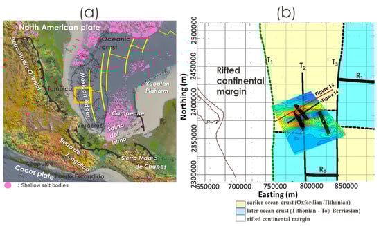
Figure 12.
Examining the deep resistivity structure of a fossil mid-ocean ridge and a possible geothermal system [11]. (a) Map showing the Mexican Ridges fold belt and the location of the 3D MT study area in the southwest of the Gulf of Mexico. The orange box is the MT study area. The yellow lines represent ridge-transform segments of the extinct Jurassic spreading center [47]. (b) Map showing the proposed ridge-transform system in the MT study area, after [48]. T1, T2, and T3 are the transform faults. R1 and R2 are the spreading ridge segments; earlier ocean crust (Oxfordian–Tithonian) and later ocean crust (Tithonian: Top Berriasian) are the proposed crustal types [48]. The embedded image is a resistivity depth slice at the top basement level from the 3D MT horizontal resistivity model [11]. The locations of the SW-NE sections in Figure 13 (red line) and Figure 14 (diamond symbols) are shown.
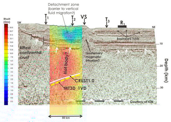
Figure 13.
Integrating seismic and MT information to identify vertical fluid migration paths and barriers [11]. Ion BasinSPAN 2D seismic PSDM data for a line crossing the survey area (green line in Figure 12b), draped by MT horizontal resistivity extracted along this line from the 3D crossgradient anisotropic MT inversion model [11]. The thick dashed yellow line is the interpreted crust-mantle interface from post-inversion electrostratigraphic imaging using the first vertical derivative (1VD) of the 3D resistivity model (see Section 2.3). The thick white line is the CRUST1.0 Moho [45]. The thick white wiggly arrows show possible seismic evidence of upward fluid migration along steep faults extending from the basement. The locations where this Ion 2D seismic line intersected features T1, T2, T3, VS (a possible volcanic seamount), and R1 (Figure 12b) are indicated at the top. MT stations are indicated by grey bars on the seafloor.
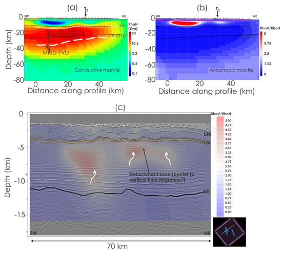
Figure 14.
Integrating information from 3D anisotropic MT models and 3D seismic data to verify vertical fluid migration paths and barriers. (a) Lithospheric horizontal resistivity section extracted along the SW-NE regional MT survey line [11]. (b) Lithospheric electrical anisotropy results were derived as the ratio of the vertical-to-horizontal resistivities along the regional line [11]. (c) Upper crustal seismic image along the regional MT line extracted from the 3D seismic cube with the resistivity anisotropy overlaid for comparison. Seismic-derived boundaries (solid black lines) and those from post-inversion electrostratigraphic imaging using the 1VD of the 3D horizontal resistivity model (white dashed lines) are shown for comparison. AB, acoustic basement. CRUST1.0 is seismic Moho [45]. The UM (Upper Miocene) and LM (Lower Miocene) are interpreted seismic horizons. Thick white wiggly arrows show possible anisotropy and seismic evidence of upward fluid migration along the steep faults extending from the basement. The other symbols are as in Figure 13. MT stations are located on the seabed (white squares and inverted black diamonds).
5. Conclusions
The search for hydrocarbon and native hydrogen reservoirs has moved to complex frontier regions where resource system fundamentals pose significant challenges, and it is critical to integrate various geophysical, geological, and environmental modeling tools in three dimensions to increase accuracy and, hence, reduce uncertainty in subsurface predictions. It is demonstrated in this paper that marine electromagnetic geophysical imaging technologies are viable components to include in this mix. By using marine data, it is shown that there could be new upside potential in reviewing legacy hydrocarbon exploration data for missed hydrogen and geothermal opportunities. These imaging technologies are also useful for geothermal energy investigations on land and, hence, could play a critical role in helping the world reach net-zero emissions by 2050.
Author Contributions
Conceptualization, M.A.M.; formal analysis, M.A.M.; investigation M.A.M.; methodology, M.A.M. and A.S.S.; software, M.A.M.; validation, M.A.M.; visualization, M.A.M.; writing—original draft, M.A.M.; writing—reviews & editing, M.A.M.; data curation, A.S.S.; funding acquisition, M.A.M. All authors have read and agreed to the published version of the manuscript.
Funding
This research received no external funding.
Data Availability Statement
The data/models re-interpreted here have been published in the publicly available literature. The software RLM3D used in the above studies was licensed by CGG Electromagnetics (Milan).
Acknowledgments
The authors are grateful to Petronas Upstream for permission to publish the various case studies drawn upon in this paper. The productive R&D collaboration with CGG Electromagnetics (Milan) is highly acknowledged.
Conflicts of Interest
The authors declare no conflict of interest.
References
- Meju, M.A. A simple geologic risk-tailored 3D controlled-source electromagnetic multiattribute analysis and quantitative interpretation approach. Geophysics 2019, 84, E155–E171. [Google Scholar] [CrossRef]
- Meju, M.A.; Gallardo, L.A. Structural-coupling approaches in integrated geophysical imaging. In Integrated Imaging of the Earth; Moorkamp, M., Lelievre, P., Linde, N., Khan, A., Eds.; AGU Books/John Wiley & Sons Inc.: Hoboken, NJ, USA, 2016; pp. 49–67. ISBN 9781118929063. [Google Scholar] [CrossRef]
- Moorkamp, M.; Heincke, B.; Jegen, M.; Hobbs, R.W.; Roberts, A.W. Joint inversion in hydrocarbon exploration. In Integrated Imaging of the Earth; Moorkamp, M., Lelievre, P., Linde, N., Khan, A., Eds.; AGU Books/John Wiley & Sons Inc.: Hoboken, NJ, USA, 2016; pp. 167–189. ISBN 9781118929063. [Google Scholar] [CrossRef]
- Meju, M.A.; Saleh, A.S.; Mackie, R.L.; Miorelli, F.; Miller, R.V.; Mansor, N.K.S. Workflow for improvement of 3D anisotropic 3D CSEM resistivity inversion and integration with seismic using cross-gradient constraint to reduce exploration risk in a complex fold-thrust belt in offshore northwest Borneo. Interpretation 2018, 6, SG49–SG57. [Google Scholar] [CrossRef]
- Gallardo, L.A.; Fontes, S.L.; Meju, M.A.; Buonora, M.P.; de Lugao, P. Robust geophysical integration through structure-coupled joint inversion and multispectral fusion of seismic reflection, magnetotelluric, magnetic and gravity images: Example from Santos Basin, offshore Brazil. Geophysics 2012, 77, B237–B251. [Google Scholar] [CrossRef]
- Gallardo, L.A.; Meju, M.A. Structure-coupled multi-physics imaging in geophysical sciences. Rev. Geophys. 2011, 49, RG1003. [Google Scholar] [CrossRef]
- Mackie, R.L.; Meju, M.A.; Miorelli, F.; Miller, R.V.; Scholl, C.; Saleh, A.S. Seismic image-guided 3D inversion of marine controlled-source electromagnetic and magnetotelluric data. Interpretation 2020, 8, SS1–SS13. [Google Scholar] [CrossRef]
- Archie, G.E. The electrical resistivity log as an aid in determining some reservoir characteristics. Trans. AIME 1942, 146, 54–62. [Google Scholar] [CrossRef]
- Eidesmo, T.; Ellingsrud, S.; MacGregor, L.M.; Constable, S.; Sinha, M.C.; Johansen, S.; Kong, S.; Westerdahl, F.N. Sea bed logging (SBL): A new method for remote and direct identification of hydrocarbon filled layers in deepwater areas. First Break 2002, 20, 144–152. [Google Scholar]
- Ellingsrud, S.; Eidesmo, T.; Johansen, S.; Sinha, M.C.; MacGregor, L.M.; Constable, S. Remote sensing of hydrocarbon layers by sea bed logging (SBL): Results from a cruise offshore Angola. Lead. Edge 2002, 21, 972–982. [Google Scholar] [CrossRef]
- Meju, M.A.; Saleh, A.S.; Karpiah, A.B.; Masnan, M.S.; Miller, R.V.; Legrand, X.; Kho, J.H.W. Three-dimensional anisotropic inversion and electrostratigraphic imaging of marine magnetotelluric data to understand the control of crustal deformation by pre-existing lithospheric structures in the Mexican Ridges Fold belt, southwestern Gulf of Mexico. Geophys. J. Int. 2023, 234, 1032–1050. [Google Scholar] [CrossRef]
- Chesley, C.; Key, K.; Constable, S.; Behrens, J.P.; MacGregor, L.M. Crustal cracks and frozen flow in oceanic lithosphere inferred from electrical anisotropy. Geochem. Geophys. Geosystems 2019, 20, 5979–5999. [Google Scholar] [CrossRef]
- Meju, M.A.; Miller, R.V.; Shukri, S.; Mansor, N.K.S.; Kho, J.H.W.; Shahar, S. Unconstrained 3D anisotropic CSEM resistivity inversion: Industry benchmark. In Proceedings of the 80th EAGE Annual Conference & Exhibition, Copenhagen, Denmark, 11–14 June; 2018. Paper Tu E 10. [Google Scholar]
- Meju, M.A.; Fatah, A. Structurally-constrained 3D anisotropic inversion of CSEM data using crossgradient criterion. In Proceedings of the 6th 3DEM International Symposium, Berkeley, CA, USA, 28–30 March 2017. [Google Scholar]
- Meju, M.A.; Mackie, R.L.; Miorelli, F.; Saleh, A.S.; Miller, R.V. Structurally-tailored 3D anisotropic CSEM resistivity inversion with cross-gradients criterion and simultaneous model calibration. Geophysics 2019, 84, E311–E326. [Google Scholar] [CrossRef]
- Hoversten, G.M.; Mackie, R.L.; Hua, Y. Reexamination of controlled-source electromagnetic inversion at the Lona prospect, Orphan Basin, Canada. Geophysics 2021, 86, E157–E170. [Google Scholar] [CrossRef]
- Saleh, A.S.; Meju, M.A.; Ismail, N.A.B.; Nawawi bin Mohd Nordin, M. Optimization of seismic-guided 3-D marine magnetotelluric imaging in a complex fold-belt setting in NW Borneo, Malaysia. Geophys. J. Int. 2022, 230, 464–479. [Google Scholar] [CrossRef]
- Karpiah, A.B.; Meju, M.A.; Saleh, A.S.; Heng, P.M.; Das, P.S.; Omar, N. Use of structure-guided 3D controlled-source electromagnetic inversion to map karst features in carbonates in offshore northwest Borneo. Geophysics 2022, 87, E279–E290. [Google Scholar] [CrossRef]
- Rose, P.R. Risk Analysis and Management of Petroleum Exploration Ventures; AAPG Methods in Exploration Series; American Association of Petroleum Geologists: Tulsa, OK, USA, 2001; 164p. [Google Scholar]
- del Real, P.G.; Vishal, V. Mineral Carbonation in Ultramafic and Basaltic Rocks. In Geologic Carbon Sequestration: Understanding Reservoir Behavior; Vishal, V., Singh, T.N., Eds.; Springer International Publishing: Cham, Switzerland, 2016; pp. 213–229. [Google Scholar]
- Ulrich, M.; Muñoz, M.; Boulvais, P.; Cathelineau, M.; Cluzel, D.; Guillot, S.; Picard, C. Serpentinization of New Caledonia peridotites: From depth to (sub-)surface. Contrib. Mineral. Petrol. 2020, 175, 91. [Google Scholar] [CrossRef]
- Lodhia, B.H. Hydrogen exploration: The next big thing? Preview 2022, 2022, 39–40. [Google Scholar] [CrossRef]
- Dugamin, E.; Truche, L.; Donze, F.V. Natural hydrogen exploration guide. ISRN Geonum-NST 2019, 1, 16. Available online: https://www.researchgate.net/publication/330728855_Natural_Hydrogen_Exploration_Guide (accessed on 1 December 2022).
- Albers, E.; Bach, W.; Pérez-Gussinyé, M.; McCammon, C.; Frederichs, T. Serpentinization-driven H2 production from continental break-up to mid-ocean ridge spreading: Unexpected high rates at the West Iberia Margin. Front. Earth Sci. 2021, 9, 673063. [Google Scholar] [CrossRef]
- Lefeuvre, N.; Truche, L.; Donze, F.-V.; Ducoux, M.; Barre, G.; Fakoury, R.-A.; Calassou, S.; Gaucher, E.C. Native H2 Exploration in the Western Pyrenean Foothills. Geochem. Geophys. Geosystems 2021, 22, e2021GC009917. [Google Scholar] [CrossRef]
- Etiope, G.; Samardzic, N.; Grassa, F.; Hrvatovic, H.; Miosic, N.; Skopljak, F. Methane and hydrogen in hyperalkaline groundwaters of the serpentinized Dinaride ophiolite belt, Bosnia and Herzegovina. Appl. Geochem. 2017, 84, 286–296. [Google Scholar] [CrossRef]
- Briere, D.; Jerzykiewicz, T.; Śliwiński, W. On Generating a Geological Model for Hydrogen Gas in the Southern Taoudenni Megabasin (Bourakebougou Area, Mali). Search and Discovery Article #42041 2017. In Proceedings of the AAPG/SEG International Conference & Exhibition, Barcelona, Spain, 3–6 April 2016. [Google Scholar]
- Prinzhofer, A.; Cisse, C.S.T.; Diallo, A.B. Discovery of a large accumulation of natural hydrogen in Bourakebougou (Mali). Int. J. Hydrogen Energy 2018, 43, 19315–19326. [Google Scholar] [CrossRef]
- Prinzhofer, A.; Moretti, I.; Françolin, J.; Pacheco, C.; d’Agostino, A.; Werly, J.; Rupin, F. Natural hydrogen continuous emission from sedimentary basins: The example of a Brazilian H2-emitting structure. 2019. Int. J. Hydrogen Energy 2019, 44, 5676–5685. [Google Scholar] [CrossRef]
- Lamadrid, H.M.; Rimstidt, J.D.; Schwarzenbach, E.M.; Klein, F.; Ulrich, S.; Dolocan, A.; Bodnar, R.J. Effect of water activity on rates of serpentinization of olivine. Nat. Commun. 2017, 8, 16107. [Google Scholar] [CrossRef] [PubMed]
- Cannat, M.; Sauter, D.; Lavier, L.; Bickert, M.; Momoh, E.; Leroy, S. On spreading modes and magma supply at slow and ultraslow mid-ocean ridges. Earth Planet. Sci. Lett. 2019, 519, 223–233. [Google Scholar] [CrossRef]
- Gillard, M.; Leroy, S.; Cannat, M.; Sloan, H. Margin-to-margin seafloor spreading in the eastern Gulf of Aden: A 16 Ma-long history of deformation and magmatism from seismic reflection, gravity and magnetic data. Front. Earth Sci. 2021, 9, 707721. [Google Scholar] [CrossRef]
- Toft, P.B.; Arkani-Hamed, J.; Haggerty, S.E. The effects of serpentinization on density and magnetic susceptibility: A petrophysical model. Phys. Earth Planet. Int. 1990, 65, 137–157. [Google Scholar] [CrossRef]
- Meju, M.A.; Jong, J.; Ogawa, K.; Muhtar, M.A.; Chuan, T.G.; Saleh, A.S.; Velayatham, T. Integrated evaluation of seabed geochemistry, geomicrobial, CSEM and seismic data to reduce exploration risk in deepwater Block 2F, offshore Sarawak, Malaysia. In Proceedings of the EAGE-Asian Petroleum Geoscience Conference and Exhibition, Kuala Lumpur, Malaysia, 12–13 October 2015. Extended Abstract. [Google Scholar]
- Meju, M.A.; Muhtar, M.A.; Choo, M.; Chakraborty, S.; Anuar, A.; Miller, R.V. Integration of seismic, CSEM and seabed geochemical data to reduce exploration risk in deepwater Block 2C, offshore Sarawak, Malaysia. In Proceedings of the EAGE-Asian Petroleum Geoscience Conference and Exhibition, Kuala Lumpur, Malaysia, 12–13 October; 2015. Extended Abstract. [Google Scholar]
- Karpiah, A.B.; Meju, M.A.; Miller, R.V.; Legrand, X.; Das, P.S.; Musafarudin, R.N.B.R. Crustal structure and basement-cover relationships in the Dangerous Grounds, offshore northwest Borneo, from 3D joint CSEM and MT imaging. Interpretation 2020, 8, SS97–SS111. [Google Scholar] [CrossRef]
- Gallardo, L.A.; Meju, M.A. Joint two-dimensional DC resistivity and seismic travel time inversion with cross-gradients constraints. J. Geophys. Res. 2004, 109, B03311. [Google Scholar] [CrossRef]
- Rodi, W.; Mackie, R.L. Nonlinear conjugate gradients algorithm for 2-D magnetotelluric inversion. Geophysics 2001, 66, 174–187. [Google Scholar] [CrossRef]
- Meju, M.A. Advances in structure-coupled multiphysics inversion theory. In Proceedings of the SEG Workshop on Multiphysics Imaging for Integrated Exploration and Field Development, Dubai, United Arab Emirates, 4–6 October 2016. [Google Scholar]
- Mackie, R.L. Geologically consistent inversion of geophysical data; a role for joint inversion. In Proceedings of the International Workshop on Gravity, Electrical and Magnetic Methods and Their Applications, Xi’an, China, 9–22 May 2019. [Google Scholar] [CrossRef]
- Meju, M.A. Regularized extremal bounds analysis (REBA): An approach to quantifying uncertainty in nonlinear geophysical inverse problems. Geophys. Res. Lett. 2009, 36, L03304. [Google Scholar] [CrossRef]
- Mackie, R.L.; Miorelli, F.; Meju, M.A. Practical methods for model uncertainty quantification in electromagnetic inverse problems. In Proceedings of the Expanded Abstract, SEG International Exposition and 88th Annual Meeting 2018, Anaheim, CA, USA, 14–19 October 2018. [Google Scholar] [CrossRef]
- Saleh, A.S.; Meju, M.; Mackie, R.; Andersen, E.; Ismail, N.A.; Nawawi, M. Seismic-Electromagnetic Projection attribute: Application in integrating seismic quantitative interpretation and 3D CSEM-MT broadband data inversion for robust ranking and sweet-spotting of hydrocarbon prospects in offshore NW Borneo. Geophysics 2023, in review. [Google Scholar]
- Ingram, G.M.; Chisholm, T.J.; Grant, C.J.; Hedlund, C.A.; Stuart-Smith, P.; Teasdale, J. Deepwater North West Borneo: Hydrocarbon accumulation in an active fold and thrust belt. Mar. Pet. Geol. 2004, 21, 879–887. [Google Scholar] [CrossRef]
- Laske, G.; Masters, G.; Ma, Z.; Pasyanos, M.E. CRUST1.0: An updated global model of Earth’s crust. Geophys. Res. Abstr. 2012, 14, 743. [Google Scholar]
- Hall, R. Contraction and extension in northern Borneo driven by subduction. J. Asian Sci. 2013, 76, 399–411. [Google Scholar] [CrossRef]
- Nguyen, L.A.; Mann, P. Gravity and magnetic constraints on the Jurassic opening of the oceanic Gulf of Mexico and the location and tectonic history of the Western Main transform fault along the eastern continental margin of Mexico. Interpretation 2016, 4, SC23–SC33. [Google Scholar] [CrossRef]
- Pindell, J.; Miranda, C.; Ceron, A.; Hernandez, L. Aeromagnetic map constrains Jurassic-Early Cretaceous synrift, break up, and rotational seafloor spreading history in the Gulf of Mexico. Mesozoic of the Gulf Rim and Beyond: New Progress in Science and Exploration of the Gulf of Mexico Basin. In Proceedings of the 35th Annual Gulf Coast Section SEPM Foundation Perkins-Rosen Research Conference. GCS SEPM Foundation, Houston, TX, USA, 8–9 December; 2016; pp. 123–153. [Google Scholar]
- Soyer, W.; Mackie, R.; Hallinan, S.; Pavesi, A.; Nordquist, G.; Suminar, A.; Intani, R.; Nelson, C. Geologically consistent multiphysics imaging of the Darajat geothermal steam field. First Break 2018, 36, 77–83. [Google Scholar] [CrossRef]


Disclaimer/Publisher’s Note: The statements, opinions and data contained in all publications are solely those of the individual author(s) and contributor(s) and not of MDPI and/or the editor(s). MDPI and/or the editor(s) disclaim responsibility for any injury to people or property resulting from any ideas, methods, instructions or products referred to in the content. |
© 2023 by the authors. Licensee MDPI, Basel, Switzerland. This article is an open access article distributed under the terms and conditions of the Creative Commons Attribution (CC BY) license (https://creativecommons.org/licenses/by/4.0/).