Abstract
At a former uranium mill site where tailings have been removed, prior work has determined several potential ongoing secondary uranium sources. These include locations with uranium sorbed to organic carbon, uranium in the unsaturated zone, and uranium associated with the presence of gypsum. To better understand uranium mobility controls at the site, four single-well push–pull tests (with a drift phase) were completed with the goal of deriving aquifer flow and contaminant transport parameters for inclusion in a future sitewide reactive transport model. This goes beyond the traditional use of a constant sorption distribution coefficient (Kd) and allows for the evaluation of alternative remedial injection fluids, which can produce variable Kd values. Dispersion was first removed from the resulting data to determine possible reactions before conducting reactive transport simulations. These initial analyses indicated the potential need to include cation exchange, uranium sorption, and gypsum dissolution. A reactive transport model using multiple layers to account for partially penetrating wells was completed using the PHT-USG reactive transport modeling code and calibrated using PEST. The model results quantify the hydraulic conductivity and dispersion parameters using the injected tracer concentrations. Uranium sorption, cation exchange, and gypsum dissolution parameters were quantified by comparing the simulated versus observed geochemistry. All simulations required some cation exchange and calcite equilibrium, and one simulation required gypsum dissolution to improve the model fit for calcium and sulfate. Uranium sorption parameters were not strongly influenced by the other parameter values but were highly influenced by uranium concentrations during the drift phase, with possible kinetic rate limitations. Thus, a future recommendation for such push–pull tests is to collect more geochemical data during the drift phase. The final uranium sorption parameters were within the range of values determined from prior column testing. The flow and transport parameters derived from these single-well push–pull tests will provide initial parameters for any future sitewide reactive transport model.
1. Introduction
Single-well push–pull tests (PPTs) are performed to quantify in situ aquifer reactions after the introduction of water with a different chemistry than the existing groundwater. In the push phase, a selected solution (with or without added tracers) is injected into the aquifer via a single well [1]. During the pull phase, prior injection water mixed with native groundwater is pumped from the same well, and water samples are taken for chemical analyses. Compared to laboratory batch or column experiments, PPTs investigate a larger aquifer volume without the direct removal of the aquifer solids, which can expose the solid-phase material to a different environment (i.e., atmospheric conditions) than the in situ aquifer state.
Istok [2] provides an overview of how to complete and interpret PPTs for site characterization. In addition to physical parameters (hydraulic conductivity and dispersion), more complex characterization can include analyses for sorption and retardation [3] microbial activity [4], redox reactions [5], biodegradation [6,7], and reaction rates [8,9]. Until recently, these analyses were generally completed using analytical models [3,4,8,10,11] or numerical models [12,13] that provide individual-process reactions (e.g., sorption or mineral dissolution or redox reactions) with reaction rates as constant values based on model fits to the PPT data.
Individual-process analytical or numerical models do not provide for coupled processes such as sorption–desorption, mineral dissolution–precipitation, multicomponent speciation, cation exchange, and reaction rates that can all occur at the same time. Fully coupled processes are included in more recent multicomponent geochemical reactive transport models (RTMs). Kruisdijk and van Breukelen [1] used RTMs with PPT data to evaluate nutrient fate and redox processes related to an aquifer storage and recovery system, which is the first use of a fully coupled RTM with PPT data to the authors’ knowledge.
In our study, we applied the PPT-RTM approach to evaluate uranium fate and transport in a contaminated aquifer that can experience an influx of nearby river water. The unique focus of this study is the determination of generic uranium sorption parameters that are empirically based and are independent of any specific mineral associations (e.g., iron oxyhydroxides or clays). These uranium sorption parameters were derived using the PPT-RTM approach and compare reasonably well to prior work using column tests on the same sediments. These parameters are specific to the site sediments and are required input data for future predictive RTMs that incorporate fully coupled reactive rock/water interactions. Future site-scale RTMs will allow for the determination of uranium mobility under various remedial scenarios. Thus, potential remedial fluids can be tested with modeling before implementing costly, larger-scale field efforts.
2. Site Description and Prior Analyses
A goal of the U.S. Department of Energy Office of Legacy Management (LM) Applied Studies and Technology Program (https://www.energy.gov/lm/services/applied-studies-and-technology-ast (accessed on 8 November 2022) is to evaluate various groundwater characterization techniques for use at multiple LM sites. Multiple tracer testing techniques were completed at a former uranium mill site (Grand Junction, CO, USA) to better quantify uranium dispersion parameters and mobility controls. This testing included single-well, multiple-well, and infiltration tracer testing coupled with groundwater quality analyses. This paper describes the single-well push–pull tracer testing with geochemical analyses for determining small-scale (10 m (m) or less) reactive transport parameters and builds upon the initial interpretations from Paradis et al. [14] along with column testing on sediments from the same area [15]. Ultimately, field-scale reactive transport parameters can be used in a sitewide RTM to evaluate various remedial options.
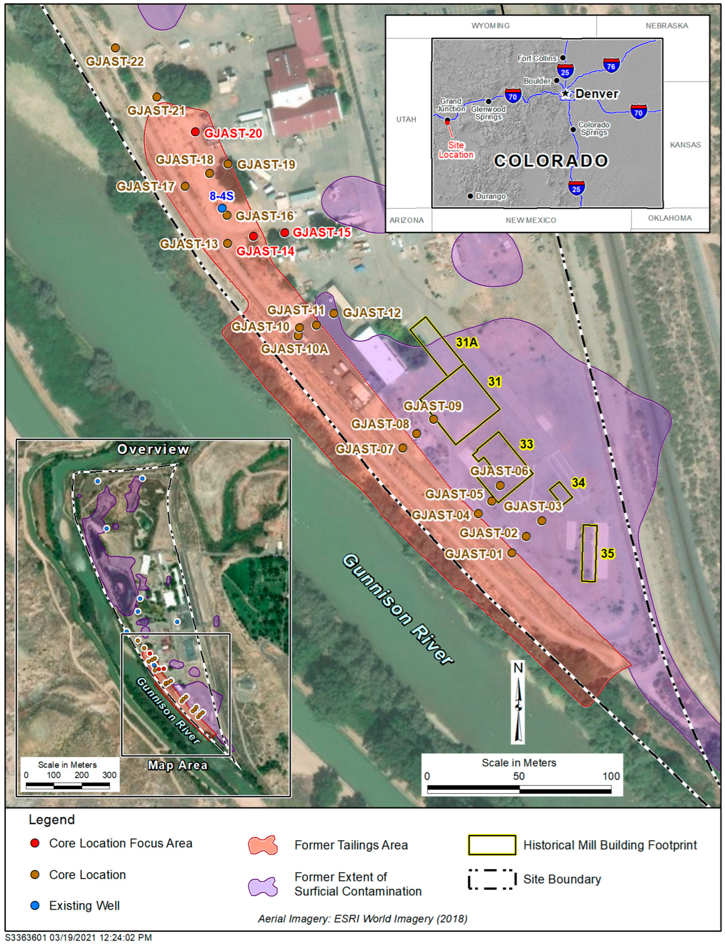
The Grand Junction, Colorado, Site (GJO) (https://www.energy.gov/lm/grand-junction-colorado-site (accessed on 8 November 2022)) is one of several legacy uranium mill sites overseen by LM for long-term surveillance and maintenance (https://www.energy.gov/lm/sites/lm-sites (accessed on 8 November 2022)). The GJO site had several uranium pilot mills operated by the U.S. Army Corps of Engineers Manhattan Engineer District from 1943 to 1958 [16]. These pilot mills were used to develop uranium extraction methods to provide uranium for the first nuclear weapons produced in the United States. Uranium tailings were deposited in low-lying areas near the pilot mills along the Gunnison River [17] (Figure 1). These tailings were present for several decades before being removed to a disposal cell [16], with excavation of contaminated material to depths that met radiological standards (radium levels below 5 picocuries per gram (pCi/g) (plus background) in the top 15 cm of sediment and below 15 pCi/g (plus background) in deeper sediment). Even though radiological standards were met, some solid-phase uranium concentrations above background were left behind [18]. Solid-phase sediments collected at multiple coring locations underneath a former tailings area in 2013 (Figure 1) identified zones with elevated uranium concentrations [15,19]. Three focus locations were used for tracer testing (Figure 1 and Figure 2), including four wells for single-well push–pull tracer tests (Figure 2) [14]. All PPTs used traced Gunnison River water as the injection solution.
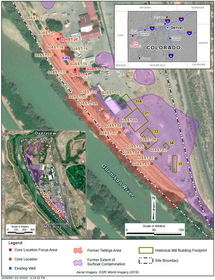
Figure 1.
GJO site with the extent of former surface contamination, former tailings area, former mill buildings, coring locations, existing wells, and three focus areas. The river is flowing northward, and the side channel is an irrigation ditch. Figure modified from Johnson et al. [15].

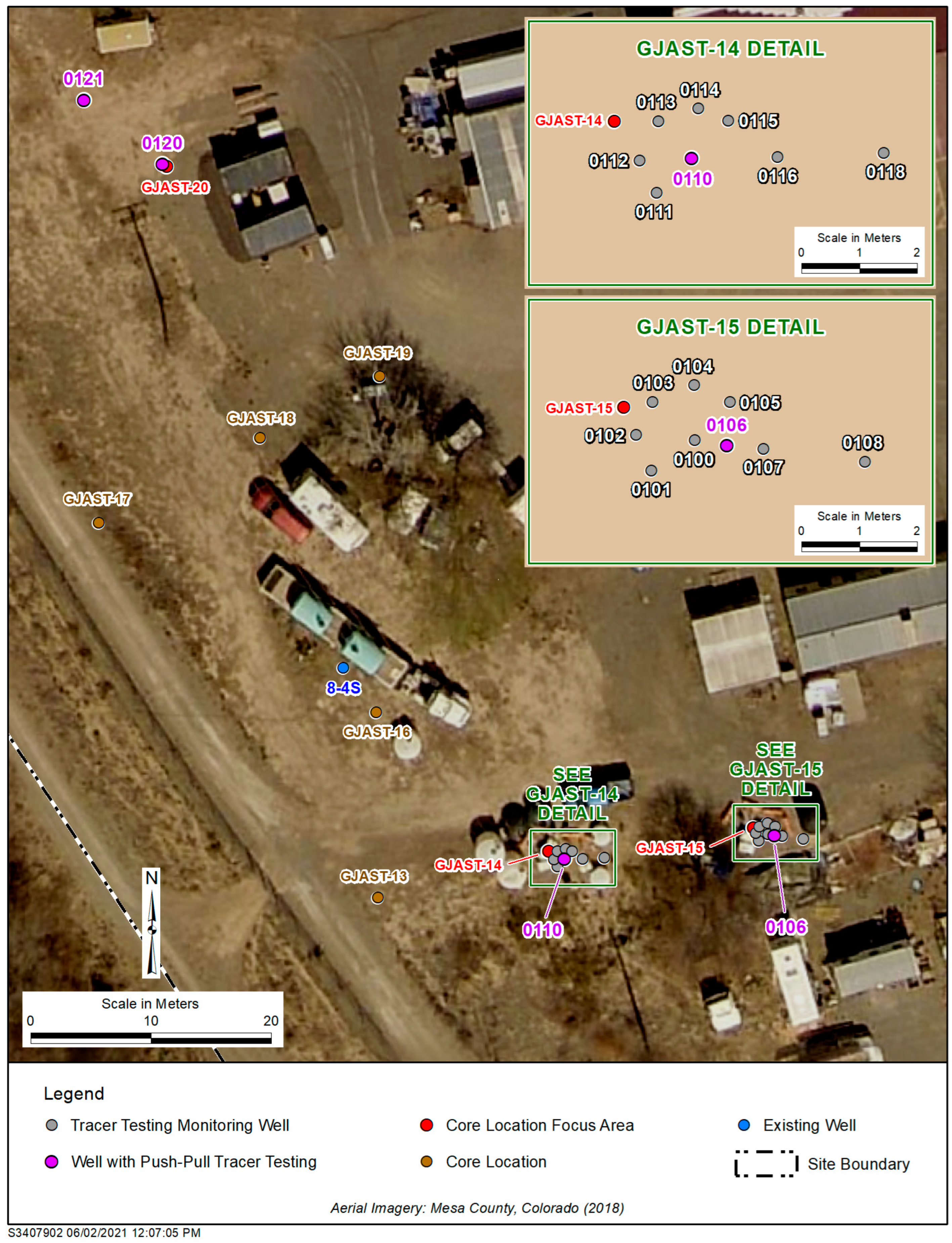
Figure 2.
GJO site around focus areas with wells installed for tracer testing. The four single-well push–pull tracer testing wells (0106, 0110, 0120, and 0121) are highlighted purple, and all other wells were used for monitoring only. Figure modified from Johnson et al. [15].
Johnson et al. [20] provides mineralogic data for uranium associations in the solid phase for some of the coring locations, and Johnson et al. [15] provides reactive transport parameters derived from column tests. The GJO site does not have a distinct groundwater uranium plume due to the changing groundwater flow directions controlled by the Gunnison River stage and the spotty nature of uranium tailings distributed in low spots across the site [21]. Recent groundwater uranium concentrations (1996 to 2021) in the area of interest (Figure 1, well 8-4S) have ranged from 0.097 to 0.73 milligrams per liter (mg/L). The GJO site is on a sand and gravel aquifer that is essentially a point bar deposit along the Gunnison River (Figure 1) with a depth of approximately 6.5 m to bedrock [19] and a typical groundwater table depth close to 3.5 m below ground surface (bgs) [15]. Groundwater flow is generally to the north–northeast and is controlled by the stage of the Gunnison River. At higher stages, groundwater flow is directly into the point-bar aquifer which reverses toward the Gunnison River at lower river stages. The groundwater table can rise up to 2.5 m at high river stages, and some groundwater inflow from the east is likely.
Paradis et al. [14] and Johnson et al. [15,20] discuss the unique uranium geochemistry on the solid phase near GJAST-14, GJAST-15, and GJAST-20 (Figure 1 and Figure 2). GJAST-14 has greater solid-phase uranium concentrations in the unsaturated zone that may be associated with evaporite mineralization. GJAST-15 has greater solid-phase uranium concentrations at and just below the water table, associated with higher organic carbon content. GJAST-20 has greater solid-phase uranium concentrations above and below the water table with column sediments indicating a consistent release of calcium and sulfate, likely associated with gypsum [15]. Single-well push–pull tracer testing was completed at well 0106 in the GJAST-15 area, at well 0110 in the GJAST-14 area, and wells 0120 and 0121 in the GJAST-20 area (Figure 2). All additional wells shown in Figure 2 were used only as monitoring wells.
3. Methods
3.1. Well Installation
All tracer testing monitoring wells and PPT wells in Figure 2 were installed with a direct-push drilling rig. Cores were collected at a few locations (wells 106, 107, 108, 116, 117, and 118) to compliment the prior coring at GJAST-14, GJAST-15, and GJAST-20. Coring could not be completed at wells 0120 or 0121 due to a dry, cemented layer at the surface that only allowed well completion. All wells were installed inside a hollow drill stem with a disposable drive point at the end. Well screens had a prepacked filter, and the formation sands and gravels collapsed around this filter up to the water table as the drill stem was withdrawn. Final annulus completion included additional silica sand followed by a bentonite seal and cement at the surface. All tracer-testing-related well completion details and boring logs are provided in Supplemental Data Folder S1. Boring logs for other GJAST locations (Figure 1) not directly discussed in this paper are provided in DOE 2018 [19].
Wells were completed in two phases. The first phase installed wells 0100 through 0105 and wells 0110 through 0115, with planned PPTs at wells 0100 and 0110 surrounded by a semicircle of monitoring wells (Figure 2). After these initial installations, fluorescein dye tracer testing was completed in wells 0100 and 0110 with monitoring in the semicircle wells to confirm the groundwater flow directions (toward wells 0102 and 0112, respectively) and quantify aquifer properties [14]. Subsequently, wells 0106, 0107, 0108, 0116, and 0118 were installed in alignment with the groundwater flow direction for use in cross-hole tracer testing. During the initial testing, it was determined that a small confining layer was creating upward flow in well 0100 [14]. Thus, wells 0106 and 0107 were installed with screens above and below this confining layer, and well 0106 was used for the PPT instead of well 0100, as originally planned. A semicircle of wells around well 0120 could not be completed due to drilling refusal and well 0121 was the nearest well that could be installed.
The 110-series wells (area with elevated solid-phase uranium in the unsaturated zone) were screened in the saturated zone at a depth of 4.0 to 5.5 m bgs. The 100-series wells (area with elevated solid-phase uranium near the water table with organic material) were screened in the saturated zone at a depth of 3.5 to 5.0 m bgs, except for well 0106 (deeper) and well 0107 (shallower) with screens at 4.7 to 5.0 and 3.8 to 4.1 m, respectively. Wells 0120 and 0121 (area with elevated solid-phase uranium across the water table and associated with gypsum) were screened within and slightly above the saturated zone at about 2.9 to 4.4 m bgs. Before the start of any PPTs, the depths to water in wells 0106, 0110, 0120, and 0121 were 3.6, 3.5, 3.4, and 3.2 m bgs, respectively. All tracer testing wells were partially penetrating in the alluvial aquifer based on well logs for GJAST-14 (110-series wells), GJAST-15 (100-series wells), and GJAST-20 (wells 0120 and 0121), where the depths to bedrock were 6.6, 6.2, and 6.3 m bgs, respectively.
3.2. Tracer Testing Procedures
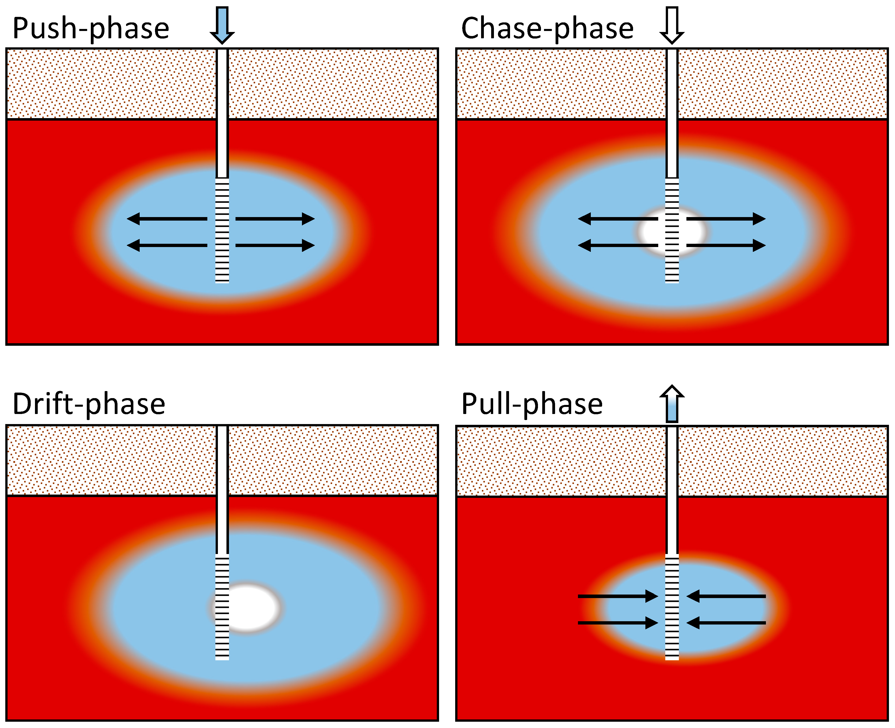
PPTs in wells 0106, 0110, 0120, and 0121 (Figure 2) were completed as push–chase–drift–pull tests (Figure 3), with the injection and pumping rates and times listed in Table 1 along with the drift time. Lower rates and volumes with a greater drift time for well 0120 (Table 1) are due to the much lower injection rate that could be achieved in this well without significant water level increases (to avoid any leaching of the unsaturated zone during PPTs). The injection solution consisted of Gunnison River water with the addition of sodium iodide and sodium 2,3,4,5,6 pentafluoro benzoate (PFB). These two tracers are considered nonreactive (conservative transport) [14] and were added to provide injection water concentrations of nearly 35 mg/L (Supplemental Data Folder S2). Iodide has a higher diffusivity than PFB [14], so the two were used together to test any aquifer dual-porosity characteristics (differential diffusion into less mobile pore spaces). In addition, chloride concentrations in the aquifer were greater than in the river water; thus, chloride could be used as a naturally occurring, conservative tracer [14].
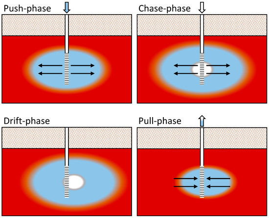
Figure 3.
Conceptual diagram of the push–chase–drift–pull approach to the PPTs. Red indicates the contaminated aquifer, blue indicates the traced Gunnison River water, and white indicates the untraced Gunnison River water. The color variation between each main color represents dispersion. The arrows highlight the injection and pumping directions with the PPT well casing (solid white) and well screen (black horizontal lines) shown in the center of each diagram. This figure follows the formatting of Kruisdijk and van Breukelen [1].

Table 1.
Push–Chase–Drift–Pull Testing Summary.
Injection of the traced river water (push phase) was followed by an injection of river water with no tracer addition (chase phase). River water injection was followed by a drift period under natural gradient conditions (drift phase). Pumping (pull phase) started just before the traced water arrived at the PPT well, which was calculated with prior groundwater flow velocity estimates and confirmed with sampling. The injected river water (traced and untraced) was pumped out until geochemical conditions returned to preinjection quality or appeared to be stable. Figure 3 conceptually shows each of the push–chase–drift–pull steps. Injection and extraction were performed using high-volume peristaltic pumps. Injection water was recirculated throughout the well screen until the injection was complete. Extraction was performed at the middle of the well screen or at the middle of the saturated interval if the water table was below the top of the well screen.
3.3. Sampling and Analyses
Injection water, prepumping groundwater, drift phase, and postpumping samples were collected at the PPT wells and monitoring wells using a peristaltic pump and dedicated plastic tubing for direct sampling. Wells 0108 and 0118 were only sampled before the push–pull testing. During pumping, 60 mL samples were continuously collected with an autosampler via a split pumping line for hourly samples. Field analyses of temperature, specific conductance, pH, oxidation–reduction potential (ORP), and dissolved oxygen (DO) were taken from the peristaltic pump line or the split pumping line (performed at least once a day, not hourly) with a field multimeter and probe (YSI 556MPS) connected to a flow-through cell. Alkalinity analyses were completed via titration. Fe2+ analyses (select nonpumping samples only) were completed with reagents added in the field and color changes measured with a spectrophotometer (Hach method 8146).
Well sampling was generally carried out from the middle of the screened interval. All samples were passed through a 0.45 micrometer filter and then split into two aliquots. One aliquot was kept at 4 °C for subsequent analyses of anions by ion chromatography (ThermoFisher Aquion ThermoFisher Scientific, Waltham, MA, USA), dissolved organic carbon (DOC) (Shimadzu TOC-L, Shimadzu, Columbia, MD, USA), iodide, and PFB by high-performance liquid chromatography (ThermoFisher Ultimate 3000, ThermoFisher Scientific, Waltham, MA, USA). The other aliquot was acidified to pH < 2 with trace-metal-grade nitric acid and subsequently analyzed for cations and metals via inductively coupled plasma–optical emission spectroscopy (ICP–OES) (Perkin Elmer DV7000, Perkin Elmer, Waltham, MA, USA) and for uranium via kinetic phosphorescence (KPA) (Chemchek KPA-11, Chemchek Instruments, Inc., Richland, WA, USA). Uranium results from the KPA were considered more accurate than uranium results from the ICP–OES analyses, and ICP–OES results for uranium below 0.1 mg/L were not used in any interpretations, albeit still considered above method detection limits. Analytical procedures followed the LM Grand Junction Environmental Sciences Laboratory (ESL) procedure manual [22].
Selected acidified samples were split for analyses at the Los Alamos National Laboratory (LANL) on an inductively coupled plasma–mass spectrometer (Perkin-Elmer NexION) with analyses for trace metals (Mo, Mn, U, Se, Sr, Li, and V). Li was included as baseline measurements for cross-hole tracer tests using LiBr (not included in this paper). The final full analyte list includes pH, temperature, specific conductance, alkalinity, DOC, Cl, NO3, SO4, I, PFB, Ca, Mg, Na, K, Fe2+, Fe, Mn, Se, U, Mo, SiO2, Sr, Li, and V. All final water quality data are provided in Supplemental Data Folder S2 in tabular and graphical formats.
3.4. Analyses for Removal of Dispersion
Paradis et al. [14] use the difference in chloride concentrations between the ambient groundwater and injected Gunnison River water as a natural, conservative tracer. This approach uses the chloride concentration differences to remove any dispersion influences for other analytes during the drift and pumping stages. Equation 1 and the graphical techniques in Paradis et al. [14] were adapted to a spreadsheet approach. This approach still uses chloride as a conservative aquifer tracer to calculate the ratio of aquifer fluids to injection fluids (e.g., a chloride concentration halfway between the aquifer and injection concentrations is 0.5, or half aquifer and half injection) that inherently accounts for dispersion. Applying this same ratio with any reactive constituent and then comparing to the chloride ratio provides a valuable method for determining possible reactions by investigating gains or losses of individual constituents (e.g., if the constituent ratio is 0.6 and chloride ratio is 0.5, then the constituent has a 0.1 or 10% gain in concentration compared to chloride). A constituent gain is removal from the solid phase to the water phase (i.e., dissolution or desorption), and a loss is a constituent transfer from the water phase to the solid phase (i.e., precipitation or sorption) with dilution influence being removed based on chloride.
Equation (1) from Paradis et al. [14] was applied to the drift portion of the PPTs at the PPT wells and surrounding ring wells as an initial step to evaluate which analytes may have undergone any chemical reactions. Using preinjection chloride concentrations and evaluating only the drift phase avoids any geochemical heterogeneities in the aquifer fluids that might be encountered during the pumping phase. This gain–loss step preceded any inverse geochemical modeling (Section 3.5 and Section 4.2.2) and, in fact, helped to inform this subsequent modeling effort.
3.5. Geochemical Modeling
Geochemical modeling was completed using PHREEQC [23] when pH, alkalinity, and all major cation and anion data were available. Using these data, plus trace metal data from the ESL or LANL, mineral saturation indices (SIs) were calculated for an extensive mineral list using the minteq.v4.dat database (available with the PHREEQC program download). PHREEQC files are provided in Supplemental Data Folder S3. Tabular and graphical results for CO2 concentrations, likely controlling minerals (calcite, gypsum, dolomite, rhodochrosite, and magnesite) and possible minerals that could control Mo, U, and V (CaMoO4, uraninite, carnotite, tyuyamunite, and Fe[VO3]2) are included in Supplemental Data Folder S2 with the water quality results. Saturation indices less than zero indicate possible mineral dissolution if that mineral exists, and SIs greater than zero indicate possible mineral precipitation. SIs near zero are considered an indicator of mineral equilibrium between the water and solid phase, within an error bound of approximately ±0.3 to account for possible analytical variability.
For all other PHREEQC modeling, an updated database (Supplemental Data Folder S4) that includes the most recent uranium thermodynamics and uranium complexation species was used [24,25]. Prior work has indicated that the use of this updated database decreases the SIs of carnotite and tyuyamunite due to the addition of calcium and magnesium uranyl carbonate complexes that keep uranium in solution [26]. Similar results occurred with the data herein by using PHREEQC with the ESL data and the updated database (Supplemental Data Folder S2 for wells 0120 and 0121; the only two wells with significant vanadium concentrations).
The inverse modeling feature of PHREEQC was used to evaluate the drift phase of the PPTs before using an RTM (Section 3.6). The inverse modeling feature in PHREEQC uses a constituent mass balance difference of final minus initial waters (i.e., postinjection drift-phase water minus preinjection groundwater) with an accounting of the differences by potential reactions provided by the user [23]. PHREEQC also allows for some analytical error which can be adjusted by the user, and pH is accounted for as a final charge balance check. The inverse modeling feature in PHREEQC can help in quantifying mineral and gas reactions along with cation exchange. However, it does not include capabilities for quantifying sorption–desorption processes.
Uranium sorption-desorption was evaluated using the generalized surface complexation modeling (GSCM) approach of Davis et al. [27]. However, the three sorption site density parameters (weak, strong, and super strong) of Davis et al. [27] were reduced to two sorption surfaces (strong (GC_s) and super strong (GC_ss)) for simplicity. The GSCM approach was used because sorption to individual components, such as iron oxides or clays, was not known or measured. The GSCM approach allows for independent variation in the sorption equilibrium constants and the sorption surface site densities. However, to avoid parameter correlation issues between the site densities and the equilibrium constants [28], only the two site densities were varied. The two site densities were consistently tied together by an order-of-magnitude difference, and the sorption equilibrium constants were held constant (5.817 and 6.798 for GC_s and GC_ss, respectively). The use of one site density parameter (GC_s) was also tested.
The PHREEQC program includes a 1D reactive transport mode [23]. However, flow velocities cannot be changed along a simulated 1D “column”. With the PPTs, flow velocities decline with expanding radial flow away from the injection wells. Thus, additional evaluations of geochemical parameters were completed using the 3D-capable reactive transport modeling approach discussed in the next section.
3.6. Reactive Transport Modeling
The reactive transport code PHT-USG was used to simulate each of the four PPTs [29]. PHT-USG couples MODFLOW-USG [30] for groundwater flow and USG-Transport [31] for contaminant transport with PHREEQC for geochemical reaction modeling capabilities. Calibration of the simulation output to the observed data used the PEST suite of software [32,33]. The graphical input/output software, Groundwater Vistas Version 8, was used for efficient model setup, simulations, calibration, and output visualization for PHT-USG and PEST. The same updated database used in the PHREEQC modeling was used in the PHT-USG modeling.
Individual RTMs were set up for each PPT. Initial groundwater flow gradients were computed using monitoring wells in the area from the time just before the tracer testing. These conditions were applied as constant head boundaries to produce the same gradient in an area around each PPT well. Cells corresponding to the test well were used to inject and pump the traced and untraced river water with the appropriate tracer concentrations and river water quality. The first calibration step used the iodide and PFB tracer data from the PPT well to estimate hydraulic conductivity and dispersivity (vertical hydraulic conductivity was tied to horizontal hydraulic conductivity at a 1:10 ratio, and transverse dispersivity was tied to longitudinal dispersivity at a 1:10 ratio). The two nonreactive tracers (iodide and PFB) had similar normalized concentrations throughout the tracer testing at all PPT wells, so dual domain issues do not look likely [14]. Both iodide and PFB were used for model calibration.
The second calibration step used U, pH, alkalinity, Ca, K, Mg, Na, and Sr data from the PPT well to estimate the uranium strong sorption site density (GC_s), calcite SI, and cation exchange capacity. Sorption sites and cation exchange sites were initialized at equilibrium with the initial groundwater chemistry. The superstrong sorption site density (GC_ss) was tied to GC_s at a 1:10 ratio, and alkalinity was entered into PHT-USG as an equivalent carbon species (C4+). Additional simulations were completed to (1) use only the strong sorption site density to simplify the parameterization and test the need for two sorption site density parameters and (2) test calibration improvement with the addition of gypsum dissolution for two wells (0120 and 0121) that had higher calcium and sulfate concentrations.
Chloride, sulfate, and silica were used in the simulations but were not used for calibration. There was some uncertainty in the ambient chloride concentrations, so the added tracers were better for calibrating the physical transport parameters. In addition, PHT-USG required the use of sulfate to charge-balance the water data in PHREEQC. For simulations that included gypsum dissolution, chloride was used to charge-balance the water data. Silica was not included in any reactions and was generally near equilibrium or slightly supersaturated with respect to chalcedony (Supplemental Data Folder S3).
Two RTMs (a 2D model and a 3D model) were created for each PPT well to test the parameter estimation differences with model layering complexity. One model assumed a single layer (fully penetrating well) and another, more representative model used multiple layers (partially penetrating well). Run times for the multilayer models were generally 40 to 50 times longer.
4. Results
4.1. Initial Groundwater and Surface Water Geochemistry
Groundwater quality for all four PPT wells was measured in triplicate just before injection occurred (Supplemental Data Folder S2). Well 0121 also had a sample taken 12 days before injection. The data in Table 2 are averages of water quality from the number of samples indicated. PPT wells 0110, 0120, and 0121 were also sampled in triplicate 1 month before injection occurred (Supplemental Data Folder S2). The differences in groundwater quality between February 2018 and March 2018 samples are minimal, except for lower iron concentrations in wells 0120 and 0121 and lower manganese concentrations in well 0110 in March 2018 (Table 2). Because PPT well 0106 was installed later than the other wells, it could not be sampled in February 2018. However, nearby wells 0100 through 0105 (Figure 2) were sampled in February 2018 (Supplemental Data Folder S2), which all show slightly greater concentrations of dissolved constituents at that time (albeit close to the limits of analytical error of around ±5%). These data indicate the potential for spatial heterogeneity in uranium and other dissolved constituents near the PPT wells. Of the four PPT wells, well 0106 appears more likely than the other PPT wells to have had a slightly different groundwater quality downgradient of the well, based on nearby sampling the month before the PPT was completed, with greater uranium, chloride, and sulfate values in wells 0100 through 0105 (Supplemental Data Folder S2; Table 2 for well 0103 as an example). The Gunnison River water that was sampled just before use as an injection fluid shows minimal differences in water quality between uses (Supplemental Data Folder S2; Table 2), and it has significantly better water quality than the groundwater, which provides a good contrast in chemistry between the groundwater and the river water (Table 2).
Table 2.
Initial Geochemistry Before Tracer Injection.
The overall geochemistry of the groundwater in each of the four PPTs wells is significantly different, especially for uranium concentrations (Table 2). As discussed in Paradis et al. [14], these differences correspond to solid-phase uranium being found in an organic-rich zone (well 0106), the vadose zone (well 0110), and a gypsum-rich zone (wells 0120 and 0121). These interpretations also correspond with column test results (15). The preinjection water quality and geochemical conditions near the PPT wells can be summarized as follows, based on the data in Table 2, data in Supplemental Data Folder S2, and information in Paradis et al. [14] and Johnson et al. [15]:
Wells 0106 and 0110 and all surrounding wells:
- Near equilibrium to slightly supersaturated with respect to calcite (SIs typically between 0.0 and 0.15).
- Typical groundwater carbon dioxide concentrations (near −1.7 log atm), which is about 2 orders of magnitude greater than the river water (near −3.5 log atm).
- Anoxic (DO typically less than 1 mg/L) to slightly reducing, measurable Mn but typically with Fe at or below detection limits. Wells 0116 and 0118 (Figure 2) are more reducing with lower ORP values and higher Mn and Fe (Supplemental Data Folder S2), possibly indicating an upgradient zone with higher organic content.
- Possible maximum solubility control on manganese by rhodochrosite in wells 0116 and 0118, with SIs of −0.17 and −0.21, respectively.
- No apparent major cation–anion control by minerals except for calcite.
- No apparent uranium mineral control (uraninite is always undersaturated) (Supplemental Data Folder S2).
- Dissolved V is generally below detection limits (0.040 mg/L).
Wells 0120 and 0121:
- Slightly supersaturated with respect to calcite (SIs typically between 0.15 and 0.30).
- Typical groundwater carbon dioxide concentrations (−1.9 to −1.7 log atm).
- Anoxic to slightly reducing (low DO and measurable Fe and Mn), and overall more reducing than wells 0106 and 0110 with more Fe and Mn and lower ORP values, but similar to wells 0116 and 0118.
- No apparent major cation–anion control by minerals except for calcite and possibly gypsum. Gypsum gets close to equilibrium saturation with an SI of −0.3 in well 0120, which corresponds to higher calcium and sulfate concentrations.
- Possible maximum solubility control on manganese by rhodochrosite, which has an SI of −0.06 for well 0120 and −0.03 for 0121.
- Higher uranium concentrations than wells 0106 and 0110 with no apparent mineral control (uraninite is always undersaturated). Likely sorption–desorption control with the possibility of uranium within the gypsum [15].
- No detectable V in well 0120 before PPT but detected during and after pumping; detectable V in well 0121 before, during, and after PPT (albeit lower V concentrations after the PPT).
Uranium mineral control by uraninite (reduced uranium mineral) was evaluated in wells 0120 and 0121 (highest uranium concentrations) using Fe2+/Fe3+ concentrations in PHREEQC (Supplemental Data Folder S3) with the updated database (Supplemental Data Folder S4). This resulted in the lowest pE being 1.6 with an associated greatest uraninite SI of −3.5 (still quite undersaturated). Using the lowest measured ORP value gives the same results and thus uraninite precipitation appears unlikely. Uranium control by carnotite and tyuyamunite was evaluated for wells 0120 and 0121 (no vanadium was detected in the other PPT wells), which resulted in SI values greater than zero for both minerals in well 0121 using the minteq.v4 database. However, using the updated database (Supplemental Data Folder S4), SI values for both carnotite and tyuyamunite in both wells are consistently less than −2.0 (Supplemental Data Folder S3). Thus, geochemical and reactive transport simulations only considered uranium concentrations that are being controlled by sorption–desorption processes. Possible uranium control by release from gypsum dissolution [15] is beyond the scope of this paper and will require additional research.
SIs for a ferrous iron vanadate mineral using both minteq.v4 and the updated database are greater than zero for well 0121. These results are similar to those at a former uranium mill site in Monticello, Utah, with elevated uranium and vanadium concentrations in the shallow groundwater [26]. At that site, vanadium appears to have a mineral (iron vanadate) and sorption control, with uranium just being sorption-controlled. At the GJO site, an excess of vanadium during pumping [14] is consistent with an iron vanadate dissolution upon oxidation. The focus of this paper is on uranium sorption parameters, but the data provided in Supplemental Data Folder S2 could be used to evaluate the controls on other site contaminants, such as vanadium and molybdenum.
4.2. Potential Reactions during PPTs
4.2.1. Analyte Gain–Loss Calculations with Dispersion Removed
Drift phase data for the PPT wells and the 100-series and 110-series semicircle ring wells (Figure 2) were evaluated using the approach discussed in Section 3.4 for the removal of dispersion (Supplemental Data Folder S5). Data for the PPT wells are provided for a specific sampling date, and the ring well data are averaged for each area (Table 3). Given potential analytical error up to 10%, a gain or loss less than 0.1 is likely not significant. Uranium shows an apparent increase, likely due to desorption from the solid phase. Silica also shows an increase compared to chloride as river water equilibrates with the aquifer solids. Nitrate behaves similarly to chloride as a conservative tracer when it is above detection limits. The ring wells have a greater loss of Ca, Mg, and Sr; a greater decrease in pH; and a greater increase in Na and K than in PPT wells 0106 and 0110 (Table 3). Compared to wells 0106 and 0110, wells 0120 and 0121 show a greater increase in calcium and sulfate, which corresponds with prior information on the possibility of gypsum in the area. Gypsum does not reach equilibrium saturation in any wells but does reach an SI of −0.8 during the drift phase in well 0120 (preinjection SI at well 0120 is −0.3).
Table 3.
Gain or Loss of Constituents to Groundwater During the Drift Phase of the PPTs Based on Chloride as a Conservative Element.
The chase water provides a useful marker to determine how much total injection water has reached a particular well. As expected, the PPT wells during the drift phase have low chloride and low iodide concentrations (chase river water), whereas the ring wells have low chloride and high iodide concentrations (traced river water). Thus, the solid phase at the PPT wells has experienced contact with river water for a longer time than the ring wells. As a result, reactions that happen quickly and reach equilibrium are more likely to have occurred already at wells 0106 and 0110 during the drift phase than the surrounding ring wells. Thus, based on Table 3, silica and uranium continue to be added to the water phase at wells 0106 and 0110 during the drift phase (likely a kinetic rate limitation), but the loss of Ca, Mg, and Sr with a gain in Na and K only occurs in the 100- and 110-series ring wells (reactions with these elements can reach equilibrium relatively quickly).
4.2.2. Quantifying Reactions with PHREEQC
The data analyses in Section 4.2.1 give quantitative gains or losses for individual constituents but do not provide specific reaction information. Thus, the inverse modeling capabilities in PHREEQC were used to quantify reactions in the drift phase, which included mineral and gas reactions and cation exchange (Supplemental Data Folder S3). Gunnison River water was the initial water and a well sample at a specific time was the final water. Chloride was used with the mixing feature in the PHREEQC inverse modeling to account for the ratio of original groundwater to river water (similar to Section 4.2.1 but performed within PHREEQC as a chloride mass balance) before evaluating any reactions.
PHREEQC inverse modeling can be very nonunique when too many constituent sources are added [23]. For example, the transfer of calcium from the solid phase to the water phase could come from cation exchange, calcite dissolution, or gypsum dissolution (likewise for Mg and Sr cation exchange and associated carbonates). Since Ca, Mg, and Sr in the 100- and 110-series ring wells have concentration losses without an associated loss of alkalinity (Table 3), carbonate mineral reactions were not included.
The final potential reaction list tested included gypsum and chalcedony mineral dissolution/precipitation, carbon dioxide speciation, and cation exchange for Na, K, Ca, Mg, and Sr. Within analytical error bounds of 5% to 10%, a mass balance was achieved with: (1) just cation exchange reactions (Ca, Mg, and Sr loss to the solid phase with a release of Na and K to the water phase) and chalcedony dissolution in the ring wells, (2) no added reactions for PPT wells 0106 and 0110, and (3) the same reactions as (1) with the addition of gypsum dissolution for PPT wells 0120 and 0121. No direct addition or loss of carbon dioxide was required, and the pH value changes for the drift-phase water was achieved by the charge balance adjustments associated with the cation exchange. For wells 0120 and 0121, Sr mass balance was achieved by cation exchange (Sr increase; Table 3), but it is suspected that Sr may also be a trace element associated with gypsum dissolution because it often substitutes for Ca. These results are consistent with the gain–loss data evaluations in Section 4.2.1 and provide a guide for specific reactions to be used in the reactive transport modeling. The identification of reactions is a necessary first step before evaluating uranium sorption parameters because uranium mobility can be highly influenced by pH along with Ca, Mg, and carbonate complexes [24].
Johnson et al. [15,20] also indicate the potential for dissolution of gypsum and silica-rich minerals, similar to the PHREEQC inverse modeling results. These previous papers suggest the potential for uranium to be associated with these gypsum and silica-rich areas (especially at well 0120) as mineral coatings. For this paper, the major uranium mobility control is considered a sorption–desorption reaction. Additional research will be required to quantify any uranium release from the dissolution of mineral coatings.
4.3. Reactive Transport Parameters Using PHT-USG
4.3.1. Results
RTM grid specifications, layering, initial conditions, boundary conditions, and time stepping details are provided in Supplemental Data Folder S6. Final calibrated model files are provided in Supplemental Data Folder S7, and the results are provided in Supplemental Data Folder S8 in a graphical format for the observed versus simulated geochemistry (iodide, PFB, Cl, SO4, U, pH, alkalinity, SiO2, Ca, K, Mg, Na, and Sr). Graphical results are presented with horizontal lines for the aquifer (dashed red) and the traced, injected river water (dashed orange) concentrations (noting that these concentrations were used in the model, which includes adjustments for charge balance in some cases for Cl and SO4). Solid black circles indicate the measured concentrations. An additional horizontal line is provided for the chase water constituent concentrations (dotted green), although they are generally the same as those of the traced water, except with no tracer concentrations. The blue solid curve lines indicate the simulated results, and a thin, pink solid curve provides the concentrations of each constituent if it behaved conservatively with no reactions. A summary of the calibrated simulation results for the estimated parameters is provided in Table 4, which are discussed in Section 4.3.2 and Section 4.3.3. Because uranium mobility can be influenced by overall water geochemistry, including pH, alkalinity, and Ca that produce various uranium complexes in solution [24], Section 4.3.4 and Section 4.3.5 discuss modeling results for constituents besides uranium first. A summary focused on the final selection of the most reasonable generic uranium sorption parameter values is provided as a separate discussion section (Section 5).
Table 4.
Estimated Parameters for Each Push–Pull Tracer Testing Well Using Single-Layer and Multilayer Modeling Approaches.
Although the actual wells are partially penetrating, the use of a single layer was evaluated to see if a simpler modeling approach with faster run times was adequate. The resulting hydraulic conductivity values for the multilayer approach are up to 2.9 times greater than the single-layer model (Table 4) but are still within prior estimates of hydraulic conductivity for the site. Prior hydraulic conductivity estimates at the GJO site range from 0.30 to 10 m per day (m/d) (0.98 to 33 feet per day (ft/d)) based on monitoring well bail testing and 12 m/d (40 ft/d) from an aquifer pumping test [17]. Dispersivity estimates for the single layer are slightly different than estimates from the multilayer approach (Table 4). No prior groundwater contaminant dispersivity estimates for the GJO site are available to the authors’ knowledge.
The single-layer approach does provide a faster calibration procedure with reasonable results for hydraulic conductivity and dispersion. However, given the differences in the uranium sorption parameters and the fact that the PPT wells are partially penetrating, the following discussions focus on the multilayer results (single layer graphical results are available in Supplemental Data Folder S8).
4.3.2. Estimated Parameter Values
The calibrated calcite SI is always positive for all models with a range from 0.10 to 0.27 (Table 4). Before the PPTs, the calcite SI ranged from −0.034 to 0.30 for all wells. Thus, the aquifer appears to have a consistent condition of being near equilibrium to slightly supersaturated with respect to calcite. During the drift phase, PHREEQC-calculated calcite SIs are larger in the PPT wells (up to 0.77), which indicates the potential for calcite to precipitate immediately after the river water injection (which had a calcite SI of up to 1.0). Currently, PHT-USG only allows for a constant mineral SI in time and space, but the gypsum SI for the injection-drift and extraction phases was varied by restarting the simulation. Estimated gypsum SIs remained negative. The cation exchange (X) parameter was comparatively low for most simulations with some variance (Table 4). For comparison, the cation exchange parameter for the saturated zone column tests at GJO ranged from 0.15 to 0.25 [15]. The uranium sorption parameters (GC_s and GC_ss) show a larger difference, especially for PPT wells 0110 and 0121 (Table 4, simulations 2 and 4, respectively). Prior estimates of these parameters at the GJO site from column testing range from 1.0 × 10⁻³ to 3.5 × 10⁻³ moles/kg-water for GC_s and 9.5 × 10⁻⁵ to 2.9 × 10⁻⁴ moles/kg-water for GC_ss [15]. These prior estimates are similar to the multilayer results with the sorption parameter range of 1.5 to 3.5 × 10⁻³ moles/kg-water for GC_s and 1.5 to 3.5 × 10⁻⁴ moles/kg-water for GC_ss for PPT wells 0106, 0110, and 0120 (Table 4, simulations 1, 2, and 3, respectively). For the well 0121 multilayer, with the inclusion of gypsum dissolution, the sorption parameters are an order of magnitude less (Table 4, simulation 4G).
A virtually identical model fit was obtained using a single sorption parameter as opposed to having two that differ by an order of magnitude (Supplemental Data Folder S8). The calibrated single sorption parameter compensates for the loss of the GC_ss parameter by increasing the GC_s parameter (Table 4, simulations 1B, 2B, 3B, and 4B).
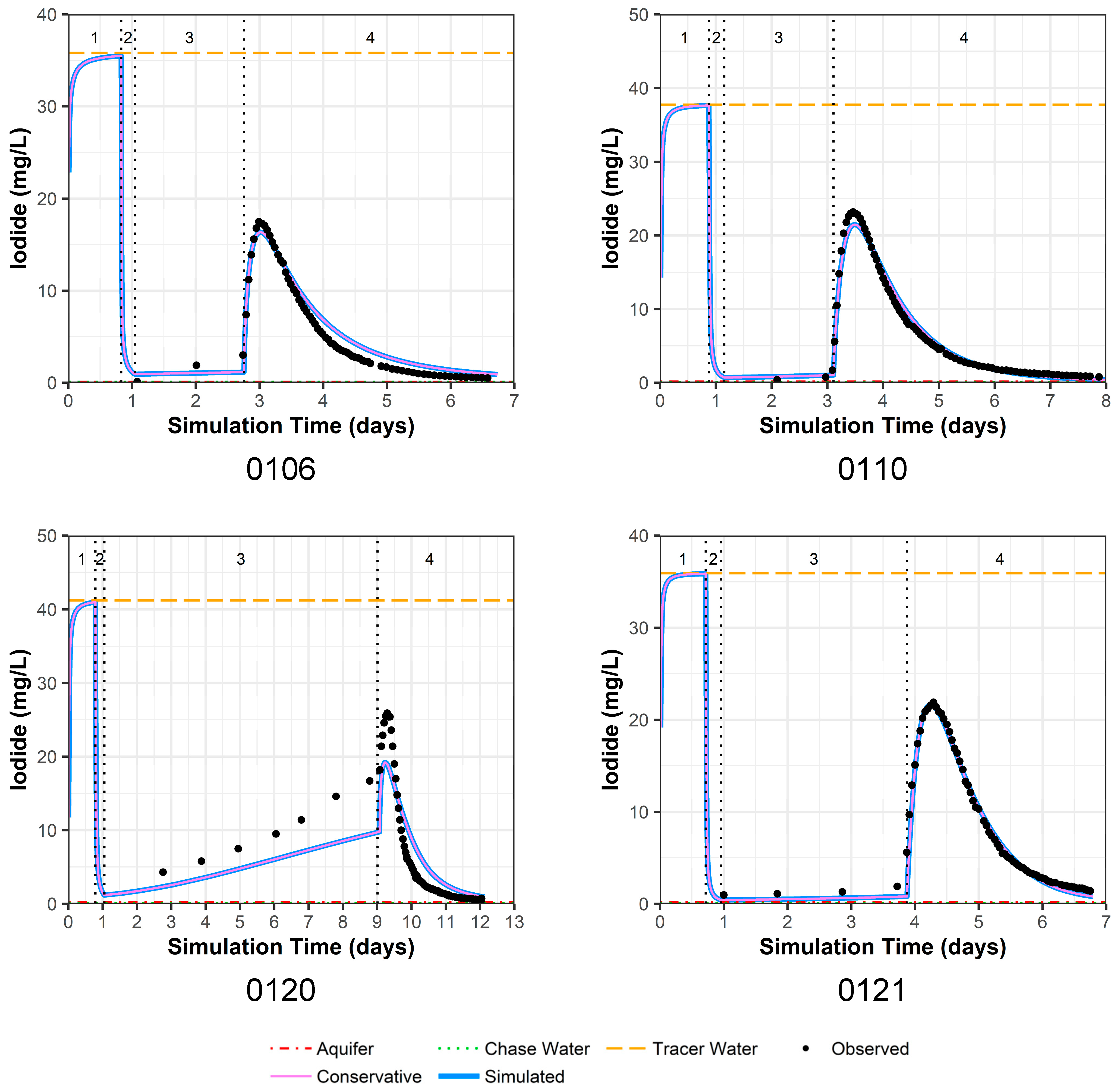
4.3.3. Iodide Model Fit
The model fit for observed versus simulated iodide concentrations for PPT wells 0106, 0110, and 0121 is very good (Figure 4). Thus, we consider the physical parameter estimates for hydraulic conductivity and dispersivity to be reasonable (Table 4). For PPT well 0120, the model fit is not as good, which is likely due to physical heterogeneity surrounding this well; this is immediately apparent because of increasing iodide seen in the drift phase (Figure 4). Such physical heterogeneity violates the model configuration of constant, surrounding hydraulic conductivity values. Larger water level responses were measured in well 0120 during pumping and injection compared to the other PPT wells, and well 0120 could not maintain the higher flow rates of the other wells (Table 1). Thus, it is likely that the bulk hydraulic conductivity around this well is lower than simulated.
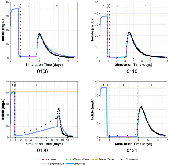
Figure 4.
Model fit for iodide in all four PPT wells with a multilayer approach. Phases are: (1) traced river water injection, (2) untraced river water injection (chase), (3) drift phase, and (4) pumping phase.
4.3.4. Model Fit for Constituents except for Uranium
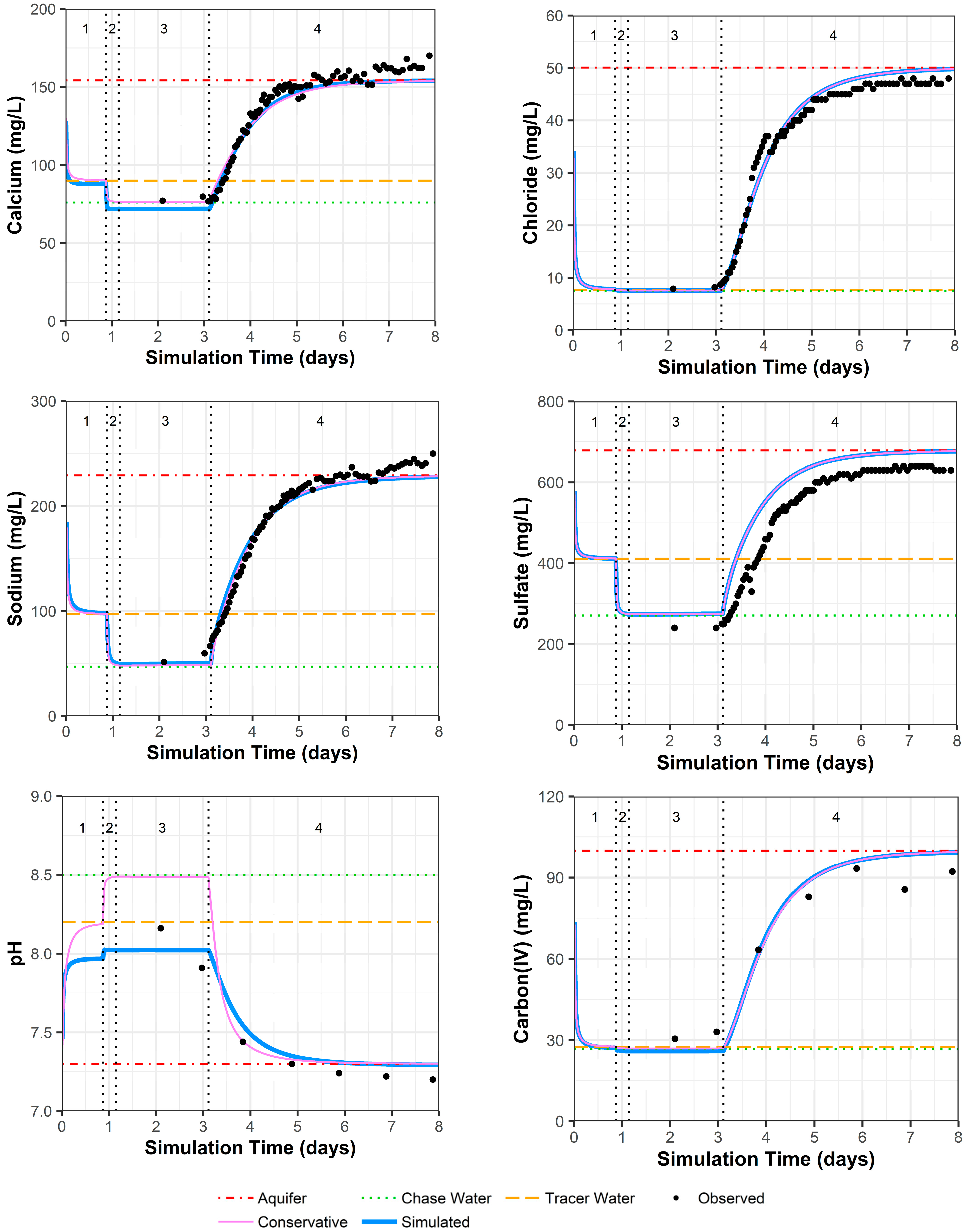
Because other constituents (especially pH and alkalinity) can influence uranium complexation, and thus the resulting sorption of uranium to the solid phase, these were examined first. PPT well 0110 shows a very good observed versus simulated fit for all constituents (Figure 5; Supplemental Data Folder S8). In Figure 5, the chase water shows a slightly different geochemistry than the traced water for calcium and sodium, which is due to one data point for the major cations in the traced water quality that may include some analytical error (Supplemental Data Folder S2). There is a small offset between the simulated and measured sulfate concentrations because sulfate was adjusted to achieve the charge balance of the solution compositions that were input to the model.
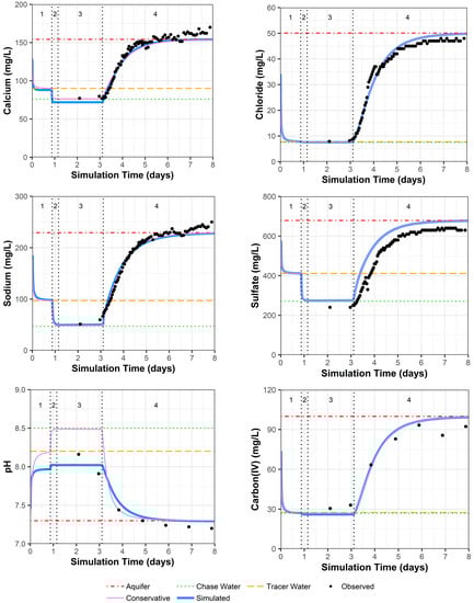
Figure 5.
Model fit for various constituents in well 0110 with a multilayer approach. Phases are: (1) traced river water injection, (2) untraced river water injection (chase), (3) drift phase, and (4) pumping phase.
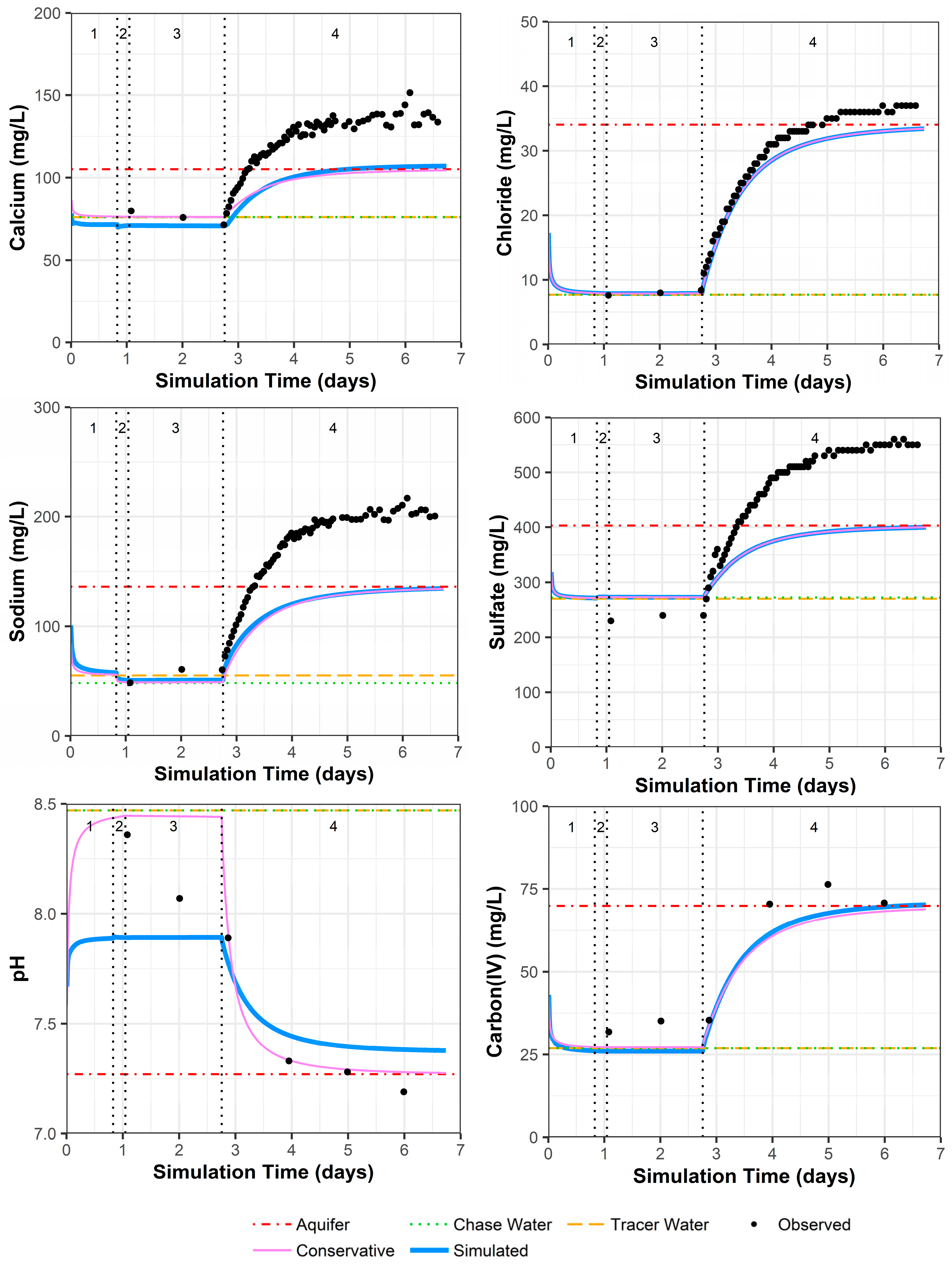
As discussed in Section 4.1, geochemical heterogeneity around PPT well 0106 can result in simulated constituent concentrations remaining lower than the observed values after pumping begins (Figure 6; for uranium, chloride, and strontium in Supplemental Data Folder S8). In addition, one of the four preinjection samples may have had low calcium, magnesium, and sodium concentration values due to analytical error that could not be reconciled (Supplemental Data Folder S2). Again, offset between the simulated and measured sulfate concentrations occurs because sulfate was adjusted to achieve the charge balance of the solution compositions that were input to the model. Although the model configuration fails to account for the surrounding geochemical heterogeneity, pH and alkalinity (the main geochemical controls on uranium) appear to have a reasonable model fit (Figure 6), with the exception that pH may have some reaction rate delays at simulation days 1 and 2.
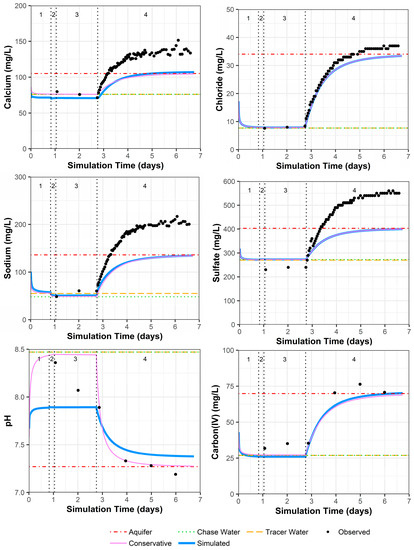
Figure 6.
Model fit for various constituents in well 0106 with a multilayer approach. Phases are: (1) traced river water injection, (2) untraced river water injection (chase), (3) drift phase, and (4) pumping phase.
4.3.5. Model Fit for Calcium and Sulfate with and without Gypsum Addition for Wells 0120 and 0121
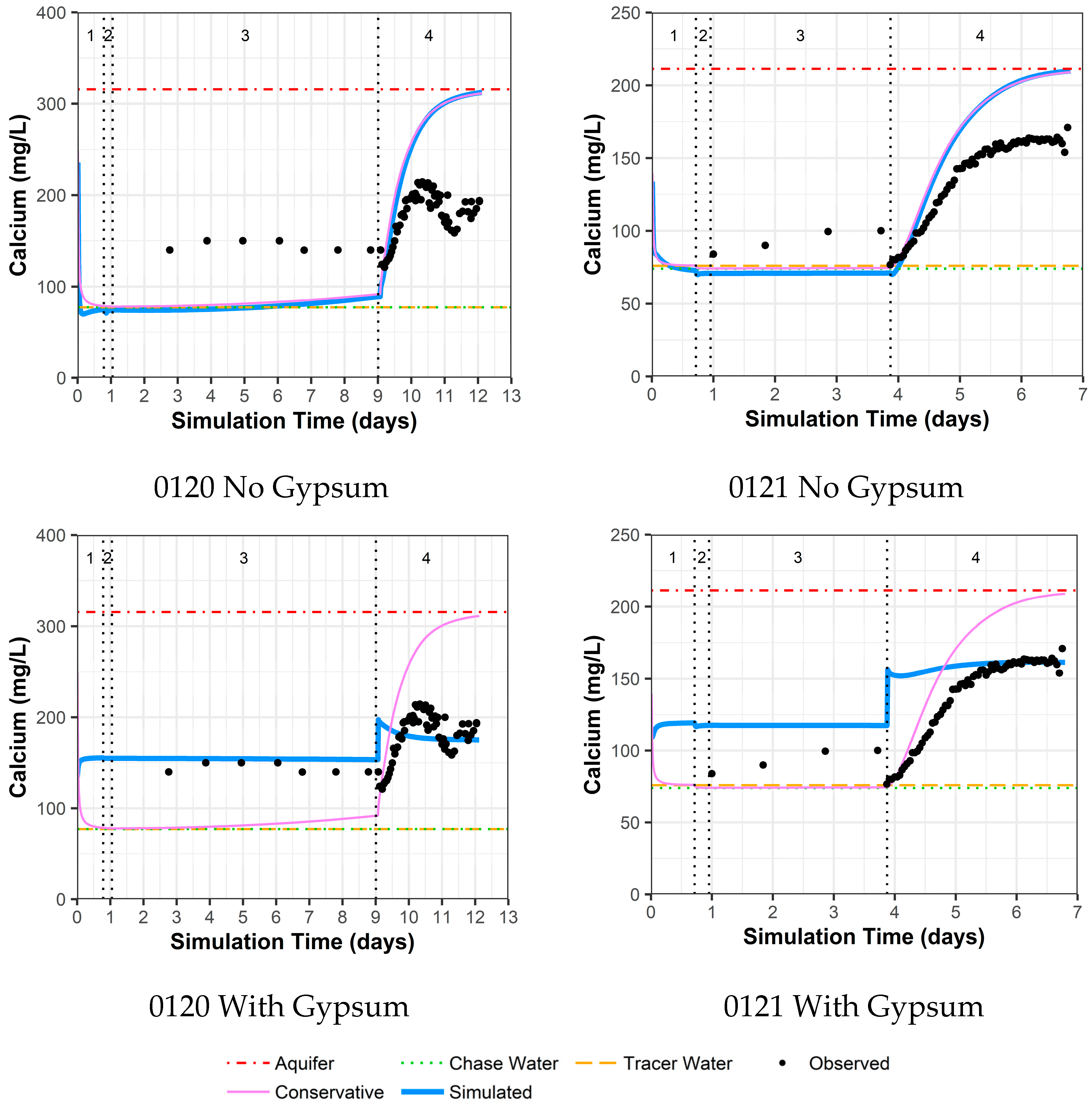
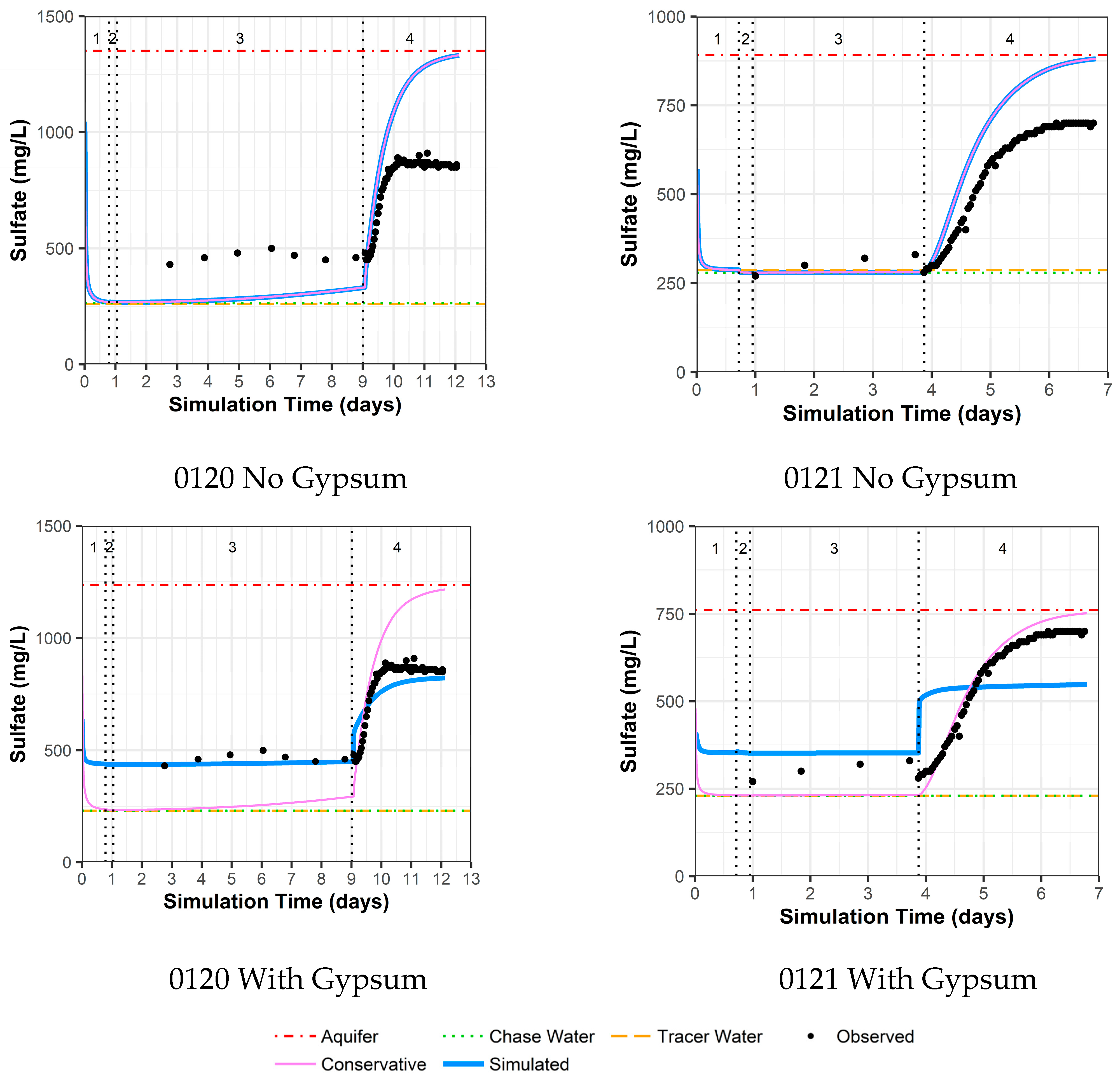
As previously mentioned, the area around wells 0120 and 0121 was identified as an area with the possible presence of gypsum. Thus, these two wells were evaluated with two models, one without the use of gypsum dissolution and one with gypsum dissolution. For well 0120 without the addition of gypsum, there are reasonable model fits to other constituents (Supplemental Data Folder S8) except for calcium, sulfate, and strontium (likely a trace element substituting for calcium within gypsum). For these constituents, the observed concentrations are higher than the simulated concentrations during the drift phase, which is then reversed during the pumping phase (Figure 7 for calcium, Figure 8 for sulfate, and Supplemental Data Folder S8 for strontium). For well 0120, the addition of gypsum to a calibrated SI of −0.80 during the injection and drift phases and −0.64 during the pumping phase dramatically improves the model fit (Figure 7 and Figure 8).
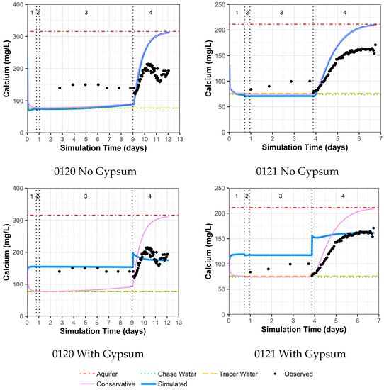
Figure 7.
Model fit for calcium with a multilayer approach. Phases are: (1) traced river water injection, (2) untraced river water injection (chase), (3) drift phase, and (4) pumping phase.
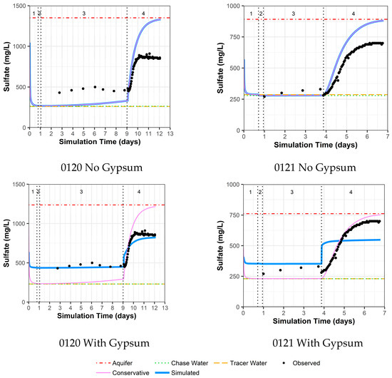
Figure 8.
Model fit for sulfate with a multilayer approach. Phases are: (1) traced river water injection, (2) untraced river water injection (chase), (3) drift phase, and (4) pumping phase.
For well 0121, the same trends as for well 0120 occurred, albeit not as large a difference between observed and simulated concentrations (Figure 7 for calcium, Figure 8 for sulfate, and Supplemental Data Folder S8 for strontium). As a result, the addition of gypsum to a calibrated SI of −0.97 during the injection and drift phases and −0.77 during the pumping phases does not produce the improvement in model fit seen for well 0120 (Figure 7 and Figure 8). However, the increased calcium and sulfate for well 0121 during the drift phase and the lower values during pumping compared to the original aquifer concentrations indicate that some gypsum dissolution might be occurring.
The addition of gypsum for well 0120 results in a calibrated decrease in the cation exchange parameter (X) and a slight increase in the uranium sorption parameter. For well 0121, the addition of gypsum slightly increases both the cation exchange and uranium sorption parameter values (Table 4).
5. Discussion of Model Fit for Uranium and Sensitivity Analyses
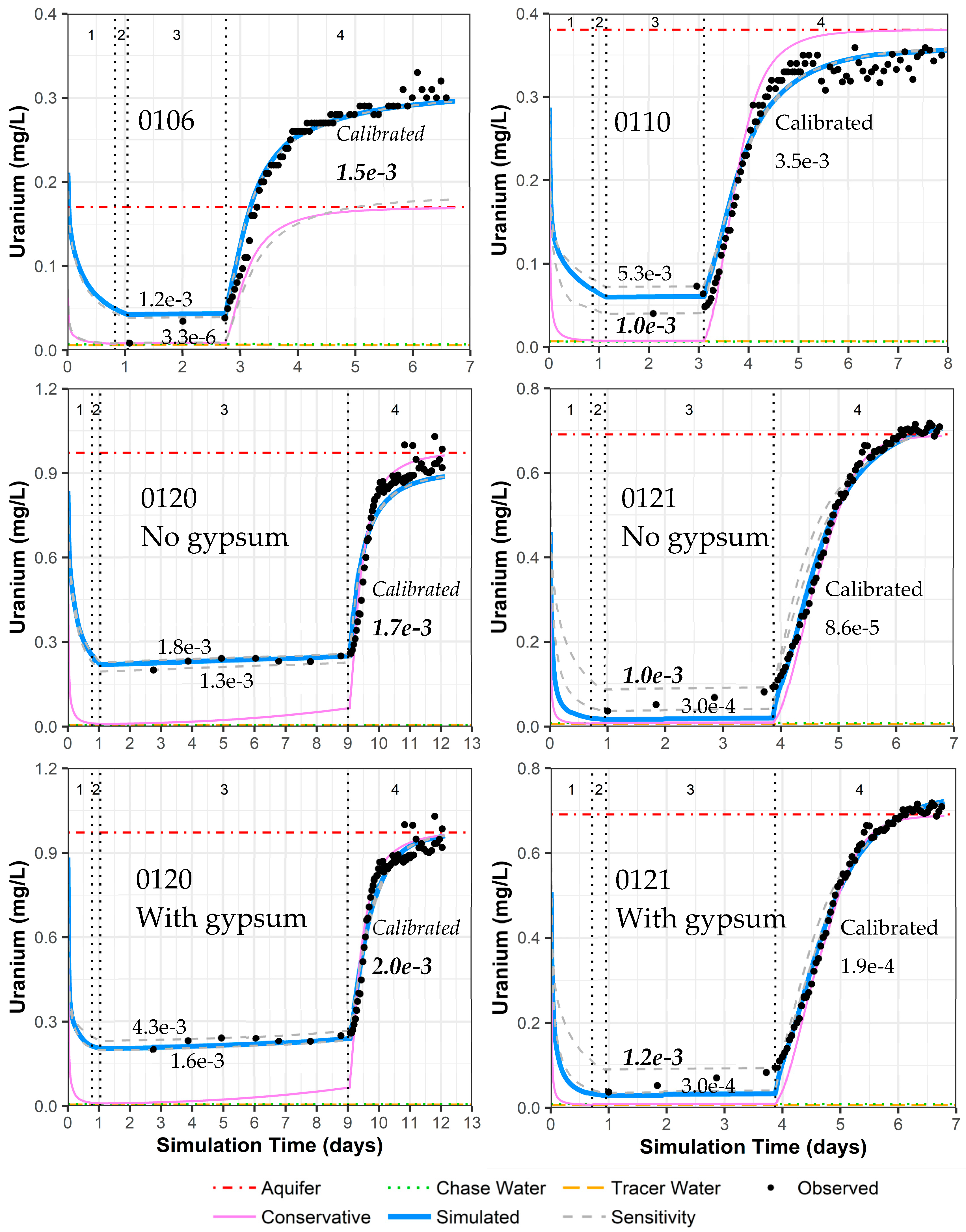
In the results section above, simulated versus measured iodide concentrations provide good model fits (Figure 4) with reasonable hydraulic conductivity and dispersion parameters (Table 4). For other constituents, each PPT well has geochemical variations that can be accounted for through the consideration of mineral dissolution/precipitation (calcite and gypsum), cation exchange, and uranium sorption/desorption (Section 4 and Table 4). This results in a good fit for the simulated versus observed uranium concentrations during the pumping phase for all of the simulations (Figure 9 and Supplemental Data Folder S8). However, the final calibrated uranium sorption parameters can vary significantly between wells based on the model fit during the drift phase, with especially low uranium sorption parameter values for well 0121 (Figure 9). To test the variation in uranium sorption parameters when fitting the concentrations during the drift phase, a sensitivity analysis was completed by fitting the model to the highest and lowest uranium concentration during the drift phase (Figure 9).
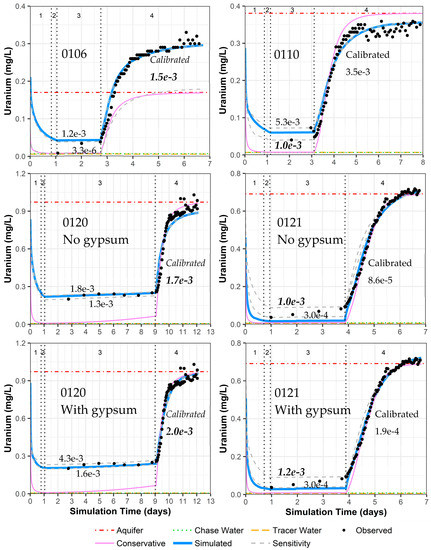
Figure 9.
Model fit for uranium in all PPT wells, with and without gypsum addition for wells 0120 and 0121. Phases are: (1) traced river water injection, (2) untraced river water injection (chase), (3) drift phase, and (4) pumping phase. Posted values are the GC_s uranium sorption parameter values (moles/kg-water) for the upper and lower sensitivity testing (gray dashed curve) and the calibrated value from Table 4 (solid blue curve). GC_s values in bold italics indicate the authors’ picks for the best final values.
Sensitivity analyses show the importance of the drift phase data in determining the uranium sorption parameters (Figure 9). For the pumping phase, the sensitivity analyses produce no change in the simulated pumping phase concentrations for wells 0110 and 0120, a change in the final aquifer concentration for well 0106, and slight curve shape differences for well 0121 (Figure 9). Relatively few data points were collected during the drift phase compared with the pumping phase, so the calibration software placed significantly more weight on matching the pumping phase data. However, a more similar sorption parameter for all the PPT wells suggests that placing more emphasis on matching the drift phase might produce more precise sorption parameter estimates. The results of the sensitivity analyses are summarized for each well simulation as follows, based on Figure 9:
- Well 0106: The drift phase is only matching two data points. Matching the lower uranium concentration in the drift phase alters the simulation to fit the aquifer uranium concentrations prior to pumping instead of the final pumping concentration (due to heterogeneity, prior discussions). Thus, the original calibration provides the most reasonable uranium sorption parameter value.
- Well 0110: There is only one data point during the middle of the drift phase and two data points just before pumping starts. It is unclear if there is some analytical error in the last two drift phase data points. The original calibration creates a fit in between the drift phase concentrations. With the sensitivity analyses, a fit to the early drift phase data creates a better fit to the early-time pumping uranium concentrations and is deemed the best simulation for deriving the most reasonable uranium sorption parameter value.
- Well 0120 without gypsum: The drift phase for this well has more data points than any other well. Thus, sensitivity analyses show only a slight change in uranium sorption parameter values. The original calibration is taken as the most reasonable uranium sorption parameter value.
- Well 0120 with gypsum: Same sensitivity results as well 0120 without gypsum, but the gypsum addition in the original calibration provides a better fit for uranium concentration during the pumping phase. The original calibration is taken as the most reasonable uranium sorption parameter value.
- Well 0121 without gypsum: The drift phase has four data points with steadily increasing uranium concentrations that cannot be simulated by the model. As such, fitting the lowest uranium concentration in the drift phase during sensitivity analyses (similar to the original calibration) likely underestimates the overall uranium sorption parameter value. Thus, fitting the larger uranium concentration in the drift phase just before pumping is selected as the best simulation for determining the most reasonable uranium sorption parameter value.
- Well 0121 with gypsum: The difference in model fit is minimal with the addition of gypsum, and the discussion is the same as the above for well 0121 without gypsum.
Although the data for wells 0106, 0110, and 0121 are limited, increasing uranium concentrations during the drift phase are not adequately simulated. This is likely due to uranium desorption kinetics that are not included in the modeling effort. The highest uranium concentrations occur at the end of the drift phase for these three wells, which does not occur in well 0120 with a much slower groundwater velocity. Although it is not typical to consider noncalibrated parameter values as the most reasonable values, possible kinetic influences that are not included in the simulations lead to a selection of uranium sorption parameter values for wells 0110 and 0121 that are not the final calibrated values (Figure 9). The difference is only a factor of 3.5 for well 0110, but it is close to an order-of-magnitude difference for well 0121. With this final selection of uranium sorption parameter values, the results are a tight range of values for GC_s from 1.0 × 10⁻³ to 2.0 × 10⁻³ moles/kg-water (GC_ss values are tied to GC_s as an order of magnitude less). These values are within the range of prior values from column testing on the same aquifer material (1.0 × 10⁻³ to 3.5 × 10⁻³ moles/kg-water for GC_s and 9.5 × 10⁻⁵ to 2.9 × 10⁻⁴ moles/kg-water for GC_ss [15]. Apparently, the inclusion of gypsum as a mineral phase has a minimal influence on the selected best uranium sorption parameter value (Figure 9), albeit that inclusion does improve model fits for calcium and sulfate, especially for well 0120 (Figure 7 and Figure 8).
6. Conclusions
Single-well push–pull tracer testing and the subsequent analyses provide a way to quantitatively determine in situ reactions in an aquifer impacted by legacy uranium mining. At the GJO site, the major reactions of cation exchange, uranium desorption, and gypsum dissolution were initially hypothesized based on constituent geochemistry after the removal of dispersion influences using chloride. These reactions were confirmed and quantified using a multilayer RTM for each of the four PPT wells.
While there are geochemical differences between the four wells in the groundwater, the final uranium sorption parameter values were similar for all four wells. This likely reflects inherent sediment similarity with respect to uranium sorption and the successful removal of any influences by groundwater geochemical differences on the inherent sorption parameter. As a result, the reactive transport modeling discussed herein can simulate the correct groundwater uranium concentrations after the existing geochemical conditions are changed. This includes perturbation of the system with the injection of river water. Final uranium sorption parameter values were also very similar to prior values derived from column testing [15]. Thus, the in situ versus ex situ testing environments and scale differences do not appear to significantly influence the uranium sorption parameter values for the GJO site. This scale independence may not occur if there are significant geochemical differences between the field and the laboratory scales (e.g., redox conditions).
Reactive transport modeling determined that the uranium sorption parameter values are more sensitive to model fitting of uranium concentrations during the drift phase than the pumping phase. Thus, a recommendation for any similar PPTs in the future is to collect more drift phase data.
The resulting reactions and quantitative parameter values from both the prior laboratory work and the field work reported herein provide input parameters that can be used in a sitewide RTM. The derivation of uranium sorption parameters for use in PHREEQC and PHT-USG provide a technique that goes beyond the traditional sorption distribution coefficient (Kd) approach, which uses a constant sorption value that does not vary with different geochemical conditions. Thus, future predictive models using PHT-USG (or another reactive transport modeling code) can adequately test remedial scenarios with various injection fluids.
Supplementary Materials
The following supporting information can be downloaded at: https://www.mdpi.com/article/10.3390/min13020228/s1, Folder S1: Well Completion Logs; Folder S2: Water Quality Data; Folder S3: PHREEQC Files; Folder S4: PHREEQC Database; Folder S5: Calculation Gain-Loss; Folder S6: PHT-USG Model Details; Folder S7: PHT-USG Model Files; Folder S8: PHT-USG Model Graphical Results.
Author Contributions
Conceptualization, R.H.J., C.J.P., A.D.T. and P.W.R.; methodology, R.H.J., C.J.P., A.D.T. and P.W.R.; software, R.D.K.; validation, A.D.T.; formal analysis, R.H.J., C.J.P., R.D.K.; investigation, R.H.J., C.J.P., A.D.T. and P.W.R.; resources, R.H.J. and A.D.T.; data curation, A.D.T.; writing—original draft preparation, R.H.J.; writing—review and editing, R.H.J., C.J.P., R.D.K., A.D.T. and P.W.R.; visualization, R.H.J. and R.D.K.; supervision, R.H.J.; project administration, R.H.J.; funding acquisition, R.H.J. All authors have read and agreed to the published version of the manuscript.
Funding
Funding for field work and laboratory analyses was provided by the U.S. Department of Energy Office of Legacy Management (LM) through contract DE-LM0000421 to Navarro Research and Engineering, Inc., as the contractor for Legacy Management Support (LMS). Funding for data analyses, modeling, and manuscript writing was provided by LM to the current LMS contractor, RSI EnTech, LLC (contract #89303020DLM000001).
Data Availability Statement
All data related to this research are provided in the Supplementary Materials.
Conflicts of Interest
The authors have no competing interest in any of this work.
References
- Kruisdijk, E.; van Breukelen, B.M. Reactive transport modelling of push-pull tests: A versatile approach to quantify aquifer reactivity. Appl. Geochem. 2021, 131, 104998. [Google Scholar] [CrossRef]
- Istok, J.D. Push-Pull Tests for Site Characterization; Springer: Berlin/Heidelberg, Germany, 2013. [Google Scholar] [CrossRef]
- Schroth, M.H.; Istok, J.D.; Haggerty, R. In situ evaluation of solute retardation using single-well push-pull tests. Adv. Water Resour. 2000, 24, 105–117. [Google Scholar] [CrossRef]
- Istok, J.D.; Humphrey, M.D.; Schroth, M.H.; Hyman, M.R.; Oreilly, K.T. Single-well, “push-pull” test for in situ determination of microbial activities. Groundwater 1997, 35, 619–631. [Google Scholar] [CrossRef]
- McGuire, J.T.; Long, D.T.; Klug, M.J.; Haack, S.K.; Hyndman, D.W. Evaluating behavior of oxygen, nitrate, and sulfate during recharge and quantifying reduction rates in a contaminated aquifer. Environ. Sci. Technol. 2002, 36, 2693–2700. [Google Scholar] [CrossRef] [PubMed]
- Kim, Y.; Istok, J.D.; Semprini, L. Push-pull tests for assessing in situ aerobic cometabolism. Groundwater 2004, 42, 329–337. [Google Scholar] [CrossRef] [PubMed]
- Michalsen, M.M.; Weiss, R.; King, A.; Gent, D.; Medina, V.F.; Istok, J.D. Push-pull test for estimating RDX and TNT degradation rates in groundwater. Groundw. Monit. Remediat. 2013, 33, 61–68. [Google Scholar] [CrossRef]
- Haggerty, R.; Schroth, M.H.; Istok, J.D. Simplified method of “push-pull” test data analysis for determining in situ reaction rate coefficients. Groundwater 1998, 36, 314–324. [Google Scholar] [CrossRef]
- Paradis, C.J.; Dixon, E.R.; Lui, L.M.; Arkin, A.P.; Parker, J.C.; Istok, J.D.; Perfet, E.; McKay, L.D.; Hazen, T.C. Improved method for estimating reaction rates during push-pull tests. Groundwater 2019, 57, 292–302. [Google Scholar] [CrossRef]
- Huang, J.; Christ, J.A.; Goltz, M.N. Analytical solutions for efficient interpretation of single-well push-pull tracer tests. Water Resour. Res. 2010, 46, W08538. [Google Scholar] [CrossRef]
- Schroth, M.H.; Istok, J.D. Approximate solution for solute transport during push-pull tests. Groundwater 2005, 43, 280–284. [Google Scholar] [CrossRef] [PubMed]
- Phanikumar, M.S.; McGuire, J.T. A multi-species reactive transport model to estimate biogeochemical rates based on single-well push-pull test data. Comput. Geosci. 2010, 36, 997–1004. [Google Scholar] [CrossRef]
- Vandenbohede, A.; Louwyck, A.; Lebbe, L. Identification and reliability of microbial aerobic respiration and denitrification kinetics using a single-well push-pull field test. J. Contam. Hydrol. 2008, 95, 42–56. [Google Scholar] [CrossRef] [PubMed]
- Paradis, C.J.; Johnson, R.H.; Tigar, A.D.; Sauer, K.B.; Marina, O.C.; Reimus, P.W. Field experiments of surface water to groundwater recharge to characterize the mobility of uranium and vanadium at a former mill tailing site. J. Contam. Hydrol. 2020, 229, 103581. [Google Scholar] [CrossRef] [PubMed]
- Johnson, R.H.; Tigar, A.D.; Richardson, C.D. Column-Test Data Analyses and Geochemical Modeling to Determine Uranium Reactive Transport Parameters at a Former Uranium Mill Site (Grand Junction, Colorado). Minerals 2022, 12, 438. [Google Scholar] [CrossRef]
- DOE (U.S. Department of Energy). Fact Sheet for the Grand Junction; Office of Legacy Management: Grand Junction, CO, USA, 2022. Available online: https://www.energy.gov/lm/articles/grand-junction-colorado-site-fact-sheet (accessed on 1 July 2022).
- DOE (U.S. Department of Energy). Final Remedial Investigation/Feasibility Study for the U.S. Department of Energy Grand Junction (Colorado) Projects Office Facility; DOE/ID/12584-16, UNC-GJ-GRAP-1; Grand Junction Office: Grand Junction, CO, USA, 1989.
- DOE (U.S. Department of Energy). Final Report of the Decontamination and Decommissioning of the Exterior Land Areas at the Grand Junction Projects Office Facility; DOE/ID/12584-220, GJPO-GJ-13; Grand Junction Office: Grand Junction, CO, USA, 1995.
- DOE (U.S. Department of Energy). Plume Persistence Final Project Report; LMS/ESL/S15233, ESL-RPT-2018-02; Office of Legacy Management: Grand Junction, CO, USA, May 2018. Available online: https://www.energy.gov/lm/services/applied-studies-and-technology-ast/ast-reports (accessed on 10 January 2022).
- Johnson, R.H.; Hall, S.M.; Tigar, A.D. Using Fission-Track Radiography Coupled with Scanning Electron Microscopy for Efficient Identification of Solid-Phase Uranium Mineralogy at a Former Uranium Pilot Mill (Grand Junction, Colorado). Geosciences 2021, 11, 294. [Google Scholar] [CrossRef]
- DOE (U.S. Department of Energy). Long-Term Surveillance and Maintenance Plan for the Grand Junction, Colorado, Site; LMS/GJT/S02013-1.0; Office of Legacy Management: Grand Junction, CO, USA, 2021.
- DOE (U.S. Department of Energy). Environmental Sciences Laboratory Procedures Manual; LMS/PRO/S04343; continuously updated; Office of Legacy Management: Grand Junction, CO, USA, 2022.
- Parkhurst, D.L.; Appelo, C.A.J. Description of Input and Examples for PHREEQC Version 3: A Computer Program for Speciation, Batch-Reaction, One-Dimensional Transport, and Inverse Geochemical Calculations. In U.S. Geological Survey Techniques and Methods; U.S. Department of the Interior: Washington, DC, USA, 2013. [Google Scholar]
- Dong, W.; Brooks, S.C. Determination of the Formation Constants of Ternary Complexes of Uranyl and Carbonate with Alkaline Earth Metals (Mg2+, Ca2+, Sr2+, and Ba2+) Using Anion Exchange Method. Environ. Sci. Technol. 2006, 40, 4689–4695. [Google Scholar] [CrossRef] [PubMed]
- Guillaumont, R.; Fanghanel, T.; Fuger, J.; Grenthe, I.; Neck, V.; Palmer, D.; Rand, M.H. Update on the Chemical Thermodynamics of Uranium, Neptunium, Plutonium, Americium and Technetium. In Chemical Thermodynamics; OECD Nuclear Energy Agency: Paris, France; Elsevier Science: Amsterdam, The Netherlands, 2003; Volume 5. [Google Scholar]
- DOE (U.S. Department of Energy). Monticello Mill Tailings Site Operable Unit III Geochemical Conceptual Site Model Update; LMS/MNT/S26486; Office of Legacy Management: Grand Junction, CO, USA, 2020. Available online: https://www.lm.doe.gov/Monticello/Documents.aspx (accessed on 1 July 2022).
- Davis, J.D.; Meece, D.E.; Kohler, M.; Curtis, G.P. Approaches to surface complexation modeling of uranium (VI) adsorption on aquifer sediments. Geochim. Cosmochim. Acta 2004, 68, 3621–3641. [Google Scholar] [CrossRef]
- Johnson, R.H.; Truax, R.A.; Lankford, D.A.; Stone, J.J. Sorption Testing and Generalized Composite Surface Complexation Models for Determining Uranium Sorption Parameters at a Proposed Uranium in situ Recovery Site. Mine Water Environ. 2016, 35, 435–446. [Google Scholar] [CrossRef]
- Panday, S.; Mori, H.; Mok, C.M.; Park, J.; Prommer, H.; Post, V. PHT-USG Module of the BTN Package of MODFLOW-USG Transport, GSI Environmental. 2019. Available online: https://www.gsienv.com/product/pht-usg-module/ (accessed on 1 July 2022).
- Panday, S.; Langevin, C.D.; Niswonger, R.G.; Ibaraki, M.; Hughes, J.D. MODFLOW–USG Version 1: An Unstructured Grid Version of MODFLOW for Simulating Groundwater Flow and Tightly Coupled Processes Using a Control Volume Finite-Difference Formulation; Techniques and Methods 6–A45; U.S. Geological Survey: Reston, VA, USA, 2013.
- Panday, S. USG-Transport Version 1.9.0: The Block-Centered Transport Process for MODFLOW-USG, GSI Environmental. 2022. Available online: https://www.gsienv.com/news/usg-transport-update/ (accessed on 15 February 2022).
- Doherty, J. Calibration and Uncertainty Analysis for Complex Environmental Models, PEST: Complete Theory and What it Means for Modeling the Real World; Watermark Numerical Computing: Brisbane, Australia, 2015; Available online: https://pesthomepage.org/pest-book (accessed on 15 January 2022).
- Doherty, J. PEST Model-Independent Parameter Estimation User Manual Part I: PEST, SENSAN and Global Optimisers, 6th ed.; Watermark Numerical Computing: Brisbane, Australia, 2016. [Google Scholar]
Disclaimer/Publisher’s Note: The statements, opinions and data contained in all publications are solely those of the individual author(s) and contributor(s) and not of MDPI and/or the editor(s). MDPI and/or the editor(s) disclaim responsibility for any injury to people or property resulting from any ideas, methods, instructions or products referred to in the content. |
© 2023 by the authors. Licensee MDPI, Basel, Switzerland. This article is an open access article distributed under the terms and conditions of the Creative Commons Attribution (CC BY) license (https://creativecommons.org/licenses/by/4.0/).