1. Introduction
Gypsum outcrops appear very frequently on the Earth’s surface and their exploitation is widespread on all continents [
1]. However, the quality and continuity of gypsum beds can vary, even under the same level of exploitation and, for this reason, its economic interest depends on the knowledge of the gypsum units that are exploited. For companies that mine gypsum, it is very important to know the thickness of the beds, as well as their continuity and purity. Additionally, gypsum usually contains detrital or carbonate materials and this can reduce its quality.
The gypsum mined is, in many cases, of secondary type; that is to say, it comes from anhydrite that is hydrated on the surface due to meteoric waters. The extent of this secondary gypsum depends on the hydration zone of the anhydrite beds from which it originates, which is not usually regular and, in many cases, does not form uniforms layers. Depending on the processes and phases of dehydration and hydration [
2], alabastrine-type nodular gypsum is associated with the gypsum of primary selenite origin with a different spatial distribution, forming veins, masses, or dispersed forms within the selenite. These different evaporitic rocks have different characteristics and markets [
3]. In addition, depending on the hydration processes, the thickness and extension of the beds of the different gypsum may considerably vary. This must be taken into account, especially for the deeper zones that are mined, since along with the depth, the number of gypsum nodular beds, created through dehydration/rehydration processes, can be more important [
4,
5].
To identify gypsum-bearing areas with an economic value, researchers use a range of approaches, from surface geological methods to advanced spaceborne thermal emission and reflection radiometer (ASTER) images [
6] in the preliminary stages of mineral exploration. However, in advanced stages of exploration, it is necessary to know the subsurface geology, and it is in these cases that core drilling is often used, which is very expensive. To optimize the exploration and exploitation of these evaporite units, relatively inexpensive techniques have been developed to help predict the continuity, purity, and presence of other rock types in these subsurface gypsum bodies, such as seismic, electrical, or electromagnetic–gravity surveys [
7,
8]. Among these techniques used for the study of gypsum outcrops, electrical resistivity tomography (ERT) has begun to be used [
9,
10,
11,
12]. This technique is gaining increasing interest, and research is being conducted on its application and usefulness in the exploration of geological resources in order to use it in the best possible way.
ERT is a geophysical prospecting method that uses electrical direct currents, which allows one to estimate the electrical resistivity distribution on the subsurface [
13]. In principle, the resistivity images obtained from the subsurface allow one to associate a lithology with each resistivity interval. However, the rock’s resistivity depends not only on the type of rock, but also on its porosity and fluid content. Porosity is affected by several factors, such as fracturing, the degree of crystallinity, and cementation [
10,
12,
14]. In addition to these factors or variables, it is necessary to bear in mind the ambiguities that can arise from the inversion of geophysical data. Therefore, it is necessary to have as much geological information as possible on the rocks under study and, in addition, to be able to obtain rock samples, borehole data, and other geophysical techniques can be integrated to develop a better interpretation of the subsurface geology, as performed in the present study.
In this study, we apply ERT and interpret the results with the help of seismic data from a given point, cores obtained from two boreholes, and surface geological information. In the study of the ERT profiles, the variability in the nature of the gypsum was considered [
9,
15] and the importance of the presence of fractures and water in the gypsum body that significantly modify the resistivity regardless of its nature is additionally highlighted. This is an important aspect to take into account since the effect of water saturation is disregarded in many studies of this type, and the influence of water is not relevant in the results presenting the low porosity and permeability of gypsum [
15].
The correlation of all these data, with the obtention of parametric measures, allows us to interpret the characteristics of the different beds of economic interest, in this case, in a specific sector of the Messinian Sorbas–Tabernas Basin (Almeria), while studying and analyzing the results obtained in the different ERT profiles to assess their usefulness.
2. Materials and Methods
In order to achieve the proposed objectives, a field study was first performed to determine the stratigraphy of the area with the gypsum unit outcrops. A geological map was created to interpret the geological structure and the relationships between the different units. For the petrographic study, some samples were collected and thin sections were created to characterize the different types of gypsum with a microscope.
Based on the study of the surface geology and data from several drill holes performed by Saint-Gobain Placo Ibérica S.A., a geophysical prospecting campaign was planned, as performed by the Geytex S.L. company, to obtain six electrical resistivity tomography (ERT) profiles. As a complementary technique, three measurements of the 1D Multichannel Analysis of Surface Waves (MASW) were performed to obtain the S-wave velocity log at a certain point. This seismic recording helped to determine the position of the boundaries of some of the gypsum banks with precision in terms of depth, since, with the geophysical exploration of electrical tomography, the determination of contrast surfaces becomes less and less precise at significant depths.
2.1. Data Acquisition Methods
2.1.1. ERT
ERT was performed by means of controlled injections of electric currents up to 1 Amp, DC. Two electrostatic devices were used: the first, of the dipole–dipole type, was used for ERT survey lines 1, 2, 3, 4, and 5, consisting of 185 m extensions with an electrostatic separation of 5 m, and 10 m long dipoles with simultaneous recording of 13 dipoles; the second, used on survey line 6, was of a composite geometry, and was a dipole–dipole + Schlumberger asymmetric type, the latter of which had current injections outside the extension at distances of 20, 40, and 60 m between the ends.
2.1.2. MASW
The seismic equipment used consisted of a digital multichannel seismograph EG&G GEOMETRICS, model GEODE, with 16 channels at 24 bits. A 110 m long seismic line with 12 geophones of a 4.5 Hz frequency and 10 m spacing was used for MASW data acquisition. The energy source was manually applied by means of the accelerated fall of an 8 kg sledgehammer from a height of 2.5 m. The position of the impact on the ground was determined by the position of the impacting ground. The position of the impact on the ground was 5 m away, outside the geophones that were placed at the ends of the line. The number of stacks used at each end of the extension was 10. The topography of the area was flat and free of environmental noise.
2.2. Data Processing
2.2.1. ERT
The inversion process and estimation of the resistivity values based on the field data and model were conducted with the assistance of the commercial software EarthImager 2D from AGI. Using this software, differences between the field values and reconstructed model can be effectively reduced (
Appendix A). The inversion of the electrical resistivity data is a non-linear iterative process that depends on a set of parameters that define the end of the iteration. The procedure we used allowed us to obtain the number of iterations, evaluate the maximum RMS error [
16,
17], and apply the L2 norm (these parameters are visible for each image at the bottom of the graphic):
The number of iterations is the maximum number of iterations (repetition of the process) for a stop in the calculation of the non-linear iterative inversion; thus, the inversion process ends when either the calculations are divergent or when there is convergence considering the preset calculation parameters.
Inversion aims to reduce the number of data mismatches between the field values and reconstructed model, i.e., the objective is to create a predicted data resistivity model that best fits the measured data. The quality of this relationship can be characterized by the root-mean-square error or RMS, expressed in %. In our case, the calculation was performed using the following expression:
where
N is the total number of measurements,
dPred represents the number of predicted data, and
dMeas represents the number of measured data.
where
N is the number of measurements,
Wi is the weight of the data,
dcalc represents the number of calculated data, and
dmeas represents the number of measured data. The L2 norm depends on the estimation of weights in the data errors and varies for each model update, a problem that is avoided by applying a norm called normalized L2 that is defined as follows:
When the normalized L2 norm is reduced to unity or becomes smaller, the inversion is said to have converged.
2.2.2. MASW
The data acquisition and processing software used was SeisImager from Geometrics. The seismic analysis was based on a robust method in the frequency domain, the CMP Cross-Correlation for Multichannel Analysis of Surface Waves (MASW), which includes the edition of quality control functions and velocity modeling.
The propagation velocity of surface waves is very close to that of an S-wave and can, therefore, be easily related [
18]. When, instead of a half-space, the behavior of a purely elastic multilayer system is analyzed, it can be observed that the phenomenon of wave propagation, on its surface, is “dispersive” and each of the frequencies
f contained in the signal, generated by the source, propagates on the surface of the system with a different velocity
c, called phase velocity, which only depends on the elastic characteristics of the different layers and the geometry of the system under consideration. The result is a change in the shape of the generated wave train (dispersion) as the signal moves away from the source [
19]. The curve relating to the phase velocity V
R is similar to V
S, with the frequency
f or the wavelength
λ, since the latter two variables are linked by the expression
c = f λ, giving rise to the dispersion curve.
The analysis we performed on the data began by establishing an initial model that we calculated as a function of the depth value. We used 1.1 times the phase velocity for an estimate of vs. and one third of the wavelength as an approximation of the depth. The minimum and maximum phase velocity values were automatically assigned based on the minimum and maximum values observed in the dispersion curve, whereas the maximum velocity was automatically assigned to the deepest layer. To calculate the vs. curve that best fits the observed data, we conducted the mathematical process of inversion, based on the method of least squares (RMS) that is applied iteratively, modifying the initial model and minimizing the difference between it and the observed data after a series of 5 iterations that, in this case, gave rise to the final model [
19], on which we represent the measured values with a green dot in each graph.
3. Geological Setting
The studied gypsum rocks, which are exploited in different areas of the region, are part of the deposits of the intermontane Sorbas Basin (post orogenic) formed in the Betic Cordillera during the Neogene (
Figure 1), in an extensional tectonic regime, e.g., [
20]. An important compressional event during the late Tortonian, possibly related to tectonic inversion of the basin [
21], caused the uplifting and erosion of the basin margins, particularly the southern one [
22]. It is in this southern zone on the southern margin of the basin that the best observations of the stratigraphy of the gypsum and its relationship with the lower units can be performed. This zone was where the study of the gypsum unit was conducted for the present work, where several studies of paleontology and stratigraphy were previously conducted, e.g., [
23,
24,
25,
26]. In general, in this sector, subhorizontal beds can be observed (0°–15° to NE) with somewhat steeper dips around the southern edge (15°–45° to S), where the Sierra Alhamilla rises (
Figure 2).
4. Stratigraphy
The stratigraphy of the Neogene Sorbas Basin, which comprises deposits from the middle Miocene to the Quaternary, is quite complex due to the variety of facies that exist, especially towards the basin rim [
27,
28]. The relationships between some of these lithological units have been frequently discussed, especially laterally, between the rim units and basin center [
22,
26]. For the Messinian, towards the center of the basin where the gypsum under study was deposited, four units can be clearly recognized, the order of which from bottom to top (
Figure 3) is the following: The Abad Member of the Turre Fm and the Yesares, Sorbas, and Zorreras members of the Caños Formation [
27,
29].
The Mb Abad is formed, mainly, by marls and silts of open sea, locally, with intercalations of diatomites in the upper part of this unit [
27,
29]. The gypsiferous member (Mb Yesares) corresponds to the marine selenitic gypsum that was deposited in the center of the basin [
30] within appropriate arid climatic and hydrological settings [
31]. The Mb Sorbas is situated with a greater variety of facies, mainly sands, silts with some carbonate levels, which have been interpreted as coastal and shallow marine facies [
32]. The coastal facies, finally, give way in the Messinian to the upper deposits of shales, sands, and conglomerates with some carbonates of continental facies (fluvial and lacustrine) of the Mb Zorreras [
32]. In the studied sector, three units were differentiated (
Figure 4):
The lower outcropping unit corresponds to the Abad Member, which consists of marls, locally with beds of diatoms, silts, and fine sands with some conglomeratic beds rich in ostreids. At some points, metric carbonate reef blocks formed by Porites were observed. Above this are the gypsum rocks that are exploited in this area (Yesares Member). The surface that separates the marls and silts from the gypsum is an irregular erosive surface, which can be related to the Messinian Mediterranean desiccation [
25,
27,
29,
33]. The existence of this erosional surface is important to consider because it may imply thickness variations in the gypsum banks, especially in the lower beds of the unit.
The gypsum unit (Yesares Member) is formed by three major gypsum banks that are separated by thin beds, a few meters thick, of marls, silts, and sands, which we called “inter-banks” (
Figure 3). The thickness of inter-banks 1 and 2 varies between 1 and 2.5 m, and inter-bank 3 is up to 6 m thick. This bank, in addition to being thicker, is more carbonated and more clearly shows marine facies. As for the three gypsum banks (G1, G2, and G3) it has been observed to have thicknesses that can vary laterally. The following thicknesses were measured for the respective banks (
Figure 4): For the G1 bank between 9 and 18 m, for the G2 bank between 24 and 28 m, and for the G3 bank between 38 and 42 m. In addition, a fourth bank (G4) outcrops in the study area, which is actually a stretch of gypsum with several detrital intercalations, where each bed of gypsum does not reach more than about 4–5 m thick, although in the easternmost drillings this bank is up to 15 m thick and with fewer detrital intercalations.
Above the gypsum unit is a second detrital unit, which we called the upper detrital unit corresponding to the Sorbas Member. This unit is formed, above all, by sands and silts. This unit is the one that covers the upper gypsum beds in the outcrops.
5. Geological Structure
In the mapped area, the four gypsum banks outcrop, with a general dip towards the NNE of about 10° (
Figure 5). The southern edge, where the gypsum disappears, is more uplifted by the thrust of Sierra Alhamilla, which is located further south (
Figure 1). The levels that served to separate the banks are the inter-banks, which are beds from 1 to 2 m of sands and silts, although sometimes they outcrop in poor conditions. From the geological cartography, quarry cuts, and cores of some boreholes, it has been possible to make a geological section approximately from SSW to NNE, as shown in
Figure 6. On the outcrops, faults and fractures in gypsum are not very visible; however, in the quarry cuts, some very fractured and broken zones can be identified, especially on the southern edge.
6. Gypsum Lithofacies
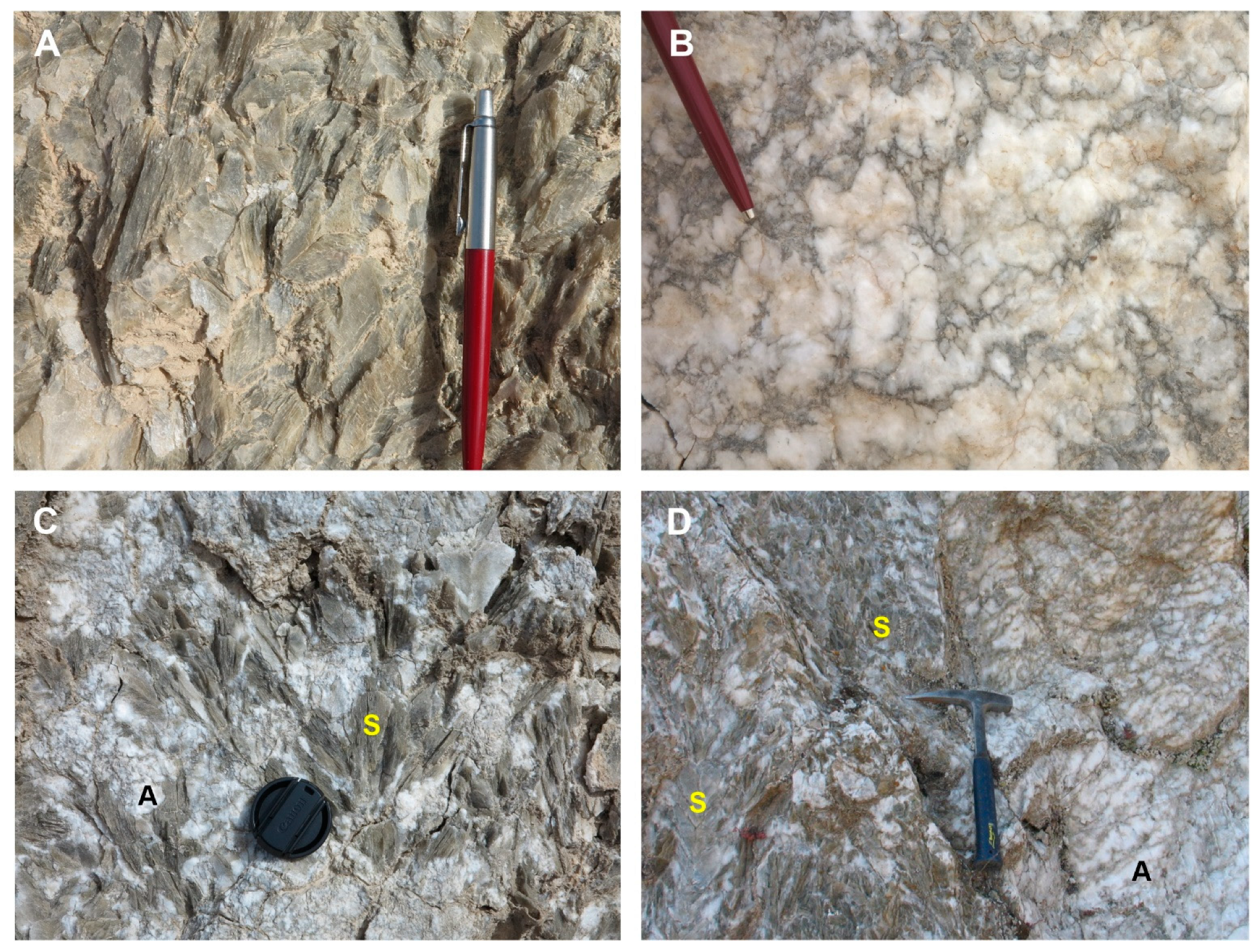
In the studied outcrops, three lithofacies can be distinguished that form part of the different gypsum levels (
Figure 7):
Macrocrystalline lithofacies, formed by selenite gypsum, are quite transparent and grayish in color, and may be formed by crystals with sizes between 1 and 25 cm in length;
Microcrystalline lithofacies, consisting of white alabastrine-type gypsum nodules, are formed by gypsum crystals smaller than one millimeter. The white nodules are bounded by a fine detrital matrix between the nodules;
The third lithofacies is of an intermediate type where large selenite crystals abound, but are surrounded by an alabastrine-type microcrystalline matrix.
The selenite gypsum is formed by transparent crystals that come from the direct precipitation of calcium sulfate that occurred in the Sorbas–Tabernas Basin during the Messinian, e.g., [
34], from brines of varying salinity rates depending on crystal sizes [
35]. The alabastrine-type gypsum is a white, microcrystalline, massive, more or less compact secondary gypsum. In addition, both types may have a matrix or fine millimetric intercalations of silts or shales.
This alabastrine gypsum usually presents nodular structures that come from the rehydration processes, which finally turn into microcrystalline gypsum, in a process that can be called the gypsification of anhydrite [
30]. Anhydrite is an anhydrous calcium sulfate mineral (CaSO
4), which when in contact with water, absorbs it and transforms into gypsum (CaSO
4-2H
2O). Therefore, anhydrite does not usually outcrop, only sometimes in the deeper zones, because it is easily rehydrated to gypsum, i.e., the anhydrite has undergone a weathering process by hydration (gypsification), giving rise to alabastrine gypsum [
36]. In this case, anhydrite comes from the dehydration of selenite when it loses a water molecule due to lithostatic pressure or the ascent of saline fluids [
5].
In the studied area, dehydration and rehydration processes are evident due to the presence of alabastrine gypsum and some very superficial structures related to the increase in volume of the crystals during dehydration. Although it is common that volume changes may not occur at all or be negligible and imperceptible [
37,
38,
39] and do not alter the structure and size of the original nodules, in the studied outcrops it is common to observe that the superficial gypsum beds locally separate from the lower beds and rise, forming a hydration relief, such as ridges and tepee-shaped structures [
36]. On the other hand, the lateral relationship between selenitic gypsum and secondary alabastrine gypsum, which comes from dehydration and rehydration processes, is visible at several points in the outcrops (
Figure 5). Sometimes, this transformation is complete throughout a bed, where only nodules of alabastrine gypsum are observed. Some other times this nodularization is clearly associated with fracture zones, as it is only distributed along a vertical fracture zone [
40] and could be associated with brines with high temperature and salinity that ascended to the surface [
41,
42,
43,
44]. It is clear that the hydration processes that lead to the formation of alabastrine gypsum can occur in the areas of the rock where water can circulate better, either through fractures, porosity, or the concentration of more or less permeable detrital materials. For this reason, a greater development of nodular alabastrine gypsum beds is observed at the base of the banks, as water can circulate better through the inter-banks.
In thin sections, under the petrographic microscope (
Figure 8), gypsum crystals with low birefringence (gray color) and very varied sizes can be observed, being very small in the case of alabastrine gypsum. It is also possible to observe in a thin section of some samples, obtained from the quarry, some dispersed anhydrite crystals that usually correspond to relict crystals that remain after a hydration phase [
40]. The presence of anhydrite was detected and quantified by some systematic chemical analyses (see Section below).
7. Lithofacies and Geochemistry Data from Borehole Cores
In the present study, we used core information from two boreholes (S13 and S14) provided by Saint-Gobain Placo Ibérica S.A. (
Figure 9). In these cores, packages 1, 2, and 3 of gypsum can be identified in both boreholes S13 and S14. The gypsum lithofacies that appear are selenite, locally with alabastrine gypsum, in the G3 bank. The G2 bank consists of alabastrine nodular gypsum and some selenite crystals. Additionally, in both the boreholes S-13 and S-14, the G1 bank is composed of alabastrine nodular gypsum.
No anhydrite beds were observed in the study area; however, their presence was detected through analysis and a thin section study (
Figure 6) of the core samples and in some quarry cuts. It is important to note in the chemical analyses of elements and minerals conducted on the core samples that, in some parts of these banks, there is a significant percentage of anhydrite, while the Cl and Na contents are also higher. The position of these zones with anhydrite and halite (ClNa) is mainly in the central parts of the banks. The highest concentrations occur in the selenitic gypsum lithofacies containing some small microcrystalline zones of secondary alabastrine gypsum. These lithofacies are found in the most central areas of the banks, which are the areas that have been away from meteoric waters for the longest time. The water involved in the sulfate hydration processes has, at the same time, been able to dissolve the ClNa associated with the original brines. Thus, the less “washed” zones are those that still have traces of anhydrite and halite.
8. Geophysical Prospection Results
8.1. Electrical Resistivity Tomography (ERT)
Six electrical tomography profiles were obtained for the study of the subsurface gypsum, showing a section representing an approximate real distribution of the resistivity measured in the subsurface [
45]. These profiles were distributed in a sector of interest outside the quarries, on its E side (
Figure 5). For their realization, the general geological structure and position of two previously performed drillings were considered.
All profiles result in relatively high resistivity values. However, the profile images show a laterally variable resistivity distribution, although the gypsum banks are more or less continuous with a very little dip.
The ERT-1 profile is very different from the rest because it presents a laterally marked discontinuity in its southern half (
Figure 10). In ERT-2, there is an important anomaly where the resistivity is quite low (<70 ohm.m) (
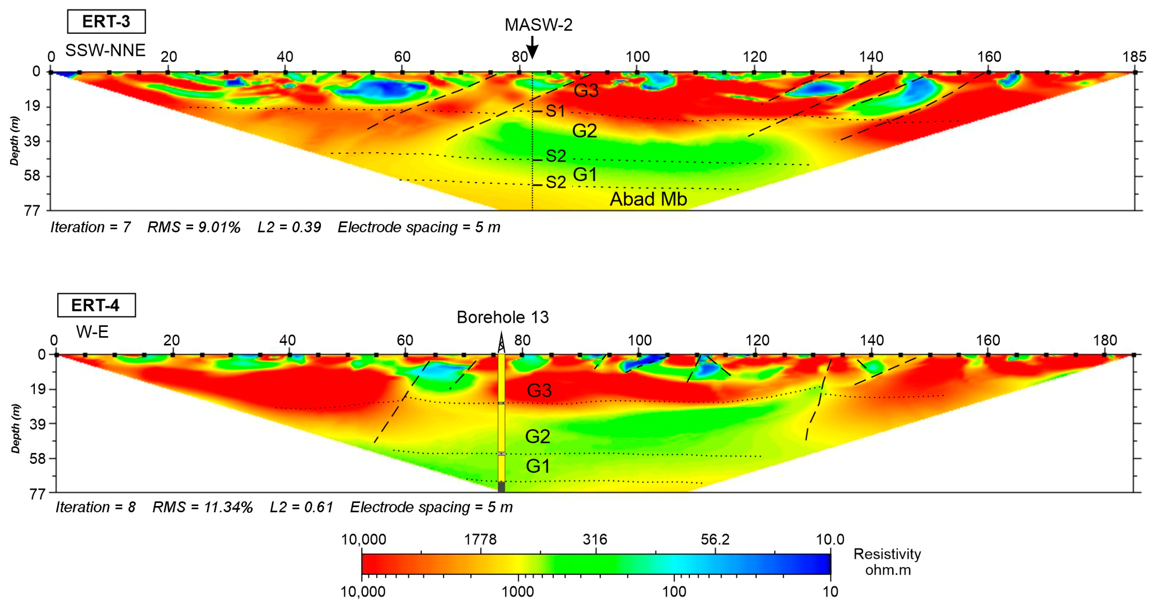
Figure 11). The ERT-3 and ERT-4 profiles are similar; both show a greater lateral continuity of resistivities with a decrease in values from a 30–35 m depth (
Figure 12). From the last section (line) studied, two profiles were obtained, which were 180 and 305 m long (
Figure 13). In the first 180 m profile (ERT-5), resistivity values were obtained of up to a 70 m depth, and in the 305 m profile (ERT-6), values were obtained for up to a 100 m depth. The most significant difference between the two profiles is that an anomaly was observed in the central zone with lower resistivity values in the deeper profile.
8.2. One-Dimensional Seismic Survey (MASW)
As an auxiliary survey technique, three 1D seismic surveys were conducted, which were located at a point within some of the ERT profiles. The propagation velocity of S-waves in gypsum can vary between 600 and 1500 m/s, according to the previous studies (
Table 1).
In the MASW-1 seismic profile (
Figure 14), a progressive velocity increase was observed up to 36–38 m in depth. The wave propagation velocity increased sharply at 22 m and decreased rapidly at 49 and 56 m depth. If we consider the average thickness of each gypsum bank, we can interpret the position of the detrital inter-banks at the indicated depths of 22 and 56 m.
The MASW-2 seismic profile after an increase in velocity shows a decrease in propagation velocities from 22–40 m depth. From 40 m, there is an increase in velocity, attenuating from 66 m onward. In these velocity changes, the approximate depth of the detrital inter-banks can be determined, taking into account the thicknesses of the gypsum banks of borehole 13. In this case, the petrographic characteristics of gypsum bank 2 (G2) indicate a disturbance in the transmission of S-waves, since they present values below 700 m/s.
The MASW-3 seismic profile shows a situation similar to the previous one. After an increase in the S-wave velocity, a sharp decrease was observed from a 33 m depth. Progressively, there is an increase in the S-wave propagation velocity with a slight decrease and stabilization at an 84 m depth. In this case, the seismic profile is next to borehole 14 and only serves to confirm that the velocity changes occur at the depths where the detrital inter-banks are located.
9. Discussion
In the geological interpretation of the subsurface, firstly, the geological structure of the area and borehole data were taken into account (
Figure 5 and
Figure 9); secondly, the electrical resistivity values attributed to the gypsum were considered. The resistivity values assigned to the lutite and different gypsum beds according to Guinea et al. 2021 (
Table 2) were used as a starting point. However, other factors that condition the resistivity and can totally modify it were also taken into account in the interpretations, such as fracturation or the presence of water in the subsurface [
9], in addition to the percolation theory [
48,
49,
50].
At some points in the ERT profiles, the entire gypsum unit (Mb Yesares), with its banks and detrital inter-banks, can be identified as a highly resistive body. In all cases, it is not possible to identify thin beds (1–5 m thick) that could have different resistivity values. This already suggests that the resistivity measurement is a total of the whole of the gypsum banks, where the inter-banks cannot be differentiated. It is evident that this occurs because of the low resolution due to the distance of the electrodes and the low thickness value of the inter-banks [
14]. In these cases, where the banks are not differentiated in the ERT profile, we can determine their thickness from the field data and borehole cores. With these data, the location of the boundaries can be further estimated using their 1D seismic profiles (
Figure 14).
The boundaries of these banks are not very well-defined in the tomography image and, sometimes, the resistivity changes do not coincide with the lithological boundaries between the different beds. Resistivity changes are determined by factors other than lithological change, such as the presence of fractures or water. In any case, the tomography image presents an average result in depth that may not coincide with the limits of the beds. In these situations, the 1D seismic survey could show us at what depth the inter-banks, which slow down the velocity of the S-waves, can be located. Where possible, a parametric was established between the 1D seismic profile and borehole core, in order to evaluate, in this case, the results of the seismic survey to corroborate its effectiveness.
Based on the geological map and the cross-sections (
Figure 1 and
Figure 6), the ERT profiles should show more continuous resistive bodies along the line (800–>5000 omh.m); however, anomalies with low resistivity (<500 omh.m) can be observed in some points or areas of the profiles, which break the lateral continuity of the highly resistive body. Different situations were observed depending on the ERT profile under study.
9.1. ERT-1 Profile
In ERT-1 to the S, there are vertical discontinuities that are very frequent: the resistive body is crossed by continuous vertical strips of lower resistivities (
Figure 10). In this case, the interpretation must be made on the basis of field observations performed on the southern edge of the outcrop. Numerous fractured or faulted zones were observed along this edge (
Figure 15). This suggests that these vertical discontinuities are due to the existence of an extensive fracture zone covering the area where the gypsum disappears by erosion to the south (
Figure 6, subsection A–A’). Fractures are filled with detrital material and water, and moisture persist longer in these shaley zones, making the resistivity of these gypsums as a whole much lower than expected. The MASW-1 profile data allow us to locate the limits of the gypsum banks in the subsurface. The Abad Mb, which shows low resistivities (<100 ohm.m), outcrops to the south.
9.2. ERT-2 Profile
In many profiles, such as ERT-2, -3, and -4, the first bank that outcrops on the surface (G3) and that can be delimited by its thickness known in outcrop and in boreholes, and corroborated by 1D seismic profiles, is the most resistive (800–>5000 ohm.m). The lower one (G2) in many cases also has a high resistivity profile, but this is not as high as that of the upper bank (300–1000 Omh-m). The lower bank (G1) may have the same or even lower resistivity values than the second bank (G2).
The ERT-2 profile is particularly significant because it presents a zone with very low resistivities (<30 ohm.m) that almost reach the surface and, supposedly, go through all the gypsum banks. It is similar to the fracture zone in the southern sector (ERT-1), but is wider and more diffuse. In this case, it is determined to be a particularly fractured zone with dissolved and accumulated clayey material. There is no surface evidence that it is a specially deformed zone. In the nearby quarry front, for example, there are no features that would imply the ascent of the Abad Mb. What we observed in other parts of the quarry were large, highly fractured areas with evidence of dissolution, sulfate precipitation, and the accumulation of shaley material, corresponding to areas through where rainwater flows (
Figure 16). This suggests that this type of zone propagates downwards and affects a large part of the gypsum banks. This more porous zone would affect the resistivity of the gypsum body, leading to low resistivity values.
9.3. ERT-3 and ERT-4 Profiles
The ERT-3 and ETR-4 profiles are almost perpendicular and located where borehole 13 was drilled (
Figure 9 and
Figure 12). According to the cores of borehole 13, the bottom of the gypsum unit (G1, G2, and G3) can be located at about a 65 m depth (ERT-4). With the help of the MASW-2 seismic test, it is possible to determine the depth where the boundaries of gypsum bank G2 reach in ERT-3. Its resistivity distribution is similar vertically: the highest resistivities occur in the upper part (>5000 ohm.m, bank G3) and at about 40 m there is a band of lower resistivity (500–700 ohm.m) that would include the G2 and G1 banks.
The G3 bank is entirely formed by selenite, while the middle–lower parts of the G2 and G1 banks are formed by nodular gypsum of alabastrine type, with a matrix between its nodules (
Figure 7 and
Figure 9). Here, one could think of this phenomenon of percolation, according to which the matrix can affect the resistivity in areas where it is abundant. As soon as the matrix is important and, above all, an interconnection is developed between the casts, a current passage can be created that lowers the resistivity of the gypsum body [
12]. Percolation theory, in the case studied, can be applied to nodular lower banks of gypsum with a shale matrix where there is a percolation threshold representing the minimum amount of shale necessary to obtain long-range connectivity [
48]. Below the percolation threshold, the electric current does not find connectivity pathways in the matrix and passes through the sulfates [
12], leading to higher resistivity values for the whole gypsum bank. However, the lithofacies of the gypsum may vary laterally, and the gypsum of the studied unit does not have important matrix contents, in general, and for this reason other alternative or complementary factors can also be considered.
Although the gypsum is very impermeable and compact, it still has some porosity due in some cases to the matrix, but mainly to the fracturing and dissolution that allows the accumulation of clay and moisture, which lowers the resistivity values to 50 ohm.m. In this type of study, it is important to consider the porosity, saturation, and interstitial fluid properties [
9]. As the matrix of this gypsum is also not very important and as the low-resistivity zone seems to be limited by faults in ERT-3 and ERT-4, it is possible that these resistivities are favored by the presence of water at a certain depth. When the resistivity drops in a whole lower zone corresponding to one of the gypsum banks, it can be interpreted that there could be a certain amount of water that would make the gypsum bank more conductive. In fact, during the electrical survey test, it was much more difficult to introduce electricity into the ground in the outcrop edge zones than in the central zone, where it could hold somewhat more water. On the other hand, as discussed, gypsum bank G1, partly G2, is formed by alabastrine gypsum nodules with some matrix, which may lower its resistivity. Microcrystalline alabastrine gypsum with a lower percentage of water can reduce resistivity more than macrocrystalline selenitic gypsum (
Figure 17).
Water will mainly flow through the fractures, depositing shaley material in them. These same fracturing and weathering processes accelerate the chemical transformation of gypsum, which leads to the rehydration of sulfates [
36]. The preferential water circulation pathways facilitate the dehydration and rehydration processes, which explains the development of alabastrine gypsum near the inter-banks and most fractured zones. The inter-banks are favorable zones for the passage of water, and therefore the zones near these detrital beds show little resistivity in the electrical prospecting tests.
9.4. ERT-5 and ERT-6 Profiles
Finally, in the easternmost sector, two overlapping profiles were developed from ERT-5 and -6. The profile for ERT-5 (180 m) shows that RMS = 3.39% is very acceptable; however, some features can be observed at greater depths in the ERT-6 profile. Similar to in other cases, in the profile for ERT-5, higher resistivity values can be observed in the upper gypsum bank (G3). At a depth of 40 m, the resistivity is below 1000 ohm.m along the entire line. This could be due to the fact that the lower banks (G1 and G2) have more nodular lithofacies. Fractures and the dissolution of gypsum result in areas with very low resistivity values (<100 ohm.m).
In the longer 305 m profile (ERT- 6), there is an anomaly of lower resistivity east of borehole 14, which could be explained by the different behavior of this low-resistivity zone due to the passage of the test current at a greater depth, which helped facilitate or find new paths in the low-resistivity zone. This passage of the current at a greater depth also produces a better visualization of what the gypsum unit (G1, G2, and G3 packages) would be, with resistivities close to 10,000 ohm.m in the central part of the profile. Therefore, the realization of these two profiles for the same section led to a better assessment of the results obtained around borehole 14, which has obviously helped in the interpretation of this section.
10. Conclusions
From the response of the different gypsum banks studied with ERT, it was observed that selenite beds have a higher resistivity than alabastrine gypsum beds. This suggests that due to the diagenetic stage, in the processes of the dehydration and rehydration of sulfates, the percolation phenomenon increases due to the redistribution of the shaley matrix in the alabastrine gypsum, decreasing its resistivity. However, the less resistive zones could be influenced by the presence of water in the subsurface, which remains in the areas with more lutite for longer, as in the more interconnected matrix, but especially, in the case of purer gypsum, in the fractures.
When the ERTs reach 70–100 m depths, the degree of detail of the resistivity variations or the definition of thin beds (<2–5 m) will be very low or null. The studied ERTs show resistivity values as a whole for banks that have detrital intercalations up to 2 m thick (inter-banks) or intervals up to 5 m thick with a relatively high anhydrite content (25%). These thin beds or intervals may lower the resistivity of the banks somewhat at their boundaries where these detrital beds are present, but in a diffuse way.
Although the purest and most compact gypsum has very high resistivity, the fracturing of the beds can fully determine the resistivity of the area of the gypsum body on which it is affected, with values below 300 ohm.m, especially when water can circulate (dissolve), introducing shale and wetting the whole area.
In the ERT tests performed, it was observed that different resistivity images could be obtained for the same section by increasing the length of the profile, which allowed the current to reach greater depths. In these cases, the variation in resistivities obtained produced several images reflecting different aspects of reality, which can present a better view of the distribution of the studied beds, if they are compared, if the similarities between these images are assumed to be more reliable data, and if objective geological data, such as borehole cores, are taken into account.
The ERT method for the study of gypsum packages can be quite time-efficient and economical. However, based on this study, it is advisable to make several profiles for the same area and to have other types of subsurface prospecting data that provide accurate references to ensure the accurate interpretation of each ERT profile that is conducted. Certain resistivity values do not always correspond to the same lithology, even for the same study area. Several local factors can modify these values: variations in the matrix content within the gypsum, the existence of thin beds of shaley material, the presence of water, fracturing, and fault or dissolution zones with detrital fill.
Author Contributions
Conceptualization, A.P.-L.; investigation, A.P.-L.; methodology, A.P.-L. and M.G.-L.; resources, M.G.-G.; software, M.G.-L.; supervision, M.G.-G.; visualization, A.P.-L.; writing—original draft, A.P.-L.; writing—review and editing, A.P.-L., M.G.-L. and M.G.-G. All authors have read and agreed to the published version of the manuscript.
Funding
This research received no external funding.
Data Availability Statement
Not applicable.
Acknowledgments
The authors would like to express their thanks to Saint-Gobain Placo Iberica, S.A., for the information and data of the study area provided for the realization of this work. Thanks are also due to the company’s personnel for the facilities provided to carry out the work, and thanks to the three anonymous reviewers for their helpful and constructive reviews of the manuscript.
Conflicts of Interest
The authors declare no conflict of interest.
Appendix A

References
- Herrero, M.J.; Escavy, J.I.; Bustillo, M. The Spanish building crisis and its effect in the gypsum quarry production (1998–2012). Resour. Policy 2013, 38, 123–129. [Google Scholar] [CrossRef]
- Ortí, F.; Rosell, L.; Salvany, J.M. Depósitos evaporíticos en España: Aspectos geológicos y recursos. In Recursos Minerales de España; García Guinea, J., Martínez Frías, J., Eds.; Textos Universitarios nº 15; CSIC: Madrid, Spain, 1992; pp. 1171–1209. [Google Scholar]
- Warren, J. Evaporites. In Their Evolution and Economics; Blackwell Science: Oxford, UK, 1999; 438p. [Google Scholar]
- Ortí, F.; Rossell, L. Evaporative systems and diagenetic patterns in the Calatayud Basin (Miocene, central Spain). Sedimentology 2000, 47, 665–685. [Google Scholar] [CrossRef]
- Ortí, F.; Rossell, L. Meganodular anhydritizacion: A new mechanism of gypsum to anhydrite conversion (Palaeogene_neogene, Ebro Basin, North-east Spain). Sedimentology 2012, 59, 1257–1277. [Google Scholar] [CrossRef]
- Habibnia, A.; Ranjbar, H.; Rahimipour, G. Gypsum exploration using ASTER data in the Hormozgan province, south of Iran. Carbonates Evaporites 2022, 37, 29. [Google Scholar] [CrossRef]
- Arjwech, R.; Everett, M.E.; Saengchomphu, S.; Somchat, K.; Pondthai, P. Geophysical mapping of gypsum for exploration of reserves in the Nong Bua area of Thailand. Q. J. Eng. Geol. Hydrogeol. 2020, 54. [Google Scholar] [CrossRef]
- Kuttikul, P.; Utha-Aroon, C.; Surinkum, A. Electromagnetic-gravity surveys: A combination for successful gypsum exploration. In Proceedings of the Ninth regional Congress on Geology, Mineral and Energy Resources of Southeast Asis—GEOSEA 1998, Kuala Lumpur, Malysia, 17–19 August 1998; pp. 17–19. [Google Scholar]
- Lugo, E.; Playà, E.; Rivero, L. Aplicación de la tomografía eléctrica a la prospección de formaciones evaporíticas. Geogaceta 2008, 44, 223–226. [Google Scholar]
- Guinea, A.; Playà, E.; Rivero, L.; Himi, M. Electrical Resistivity Tomography and Induced Polarization techniques applied to the identification of gypsum rocks. Near Surf. Geophys. 2010, 8, 249–257. [Google Scholar] [CrossRef]
- Martínez, N.; Guinea, A.; Playà, E.; Rivero, L. Estudio de viabilidad de canteras de yeso mediante tomografía eléctrica. Rocas Y Miner. 2013, 41, 20–25. Available online: http://hdl.handle.net/2445/98437 (accessed on 10 January 2023).
- Guinea, A.; Playà, E.; Rivero, L.; Ledo, J.J.; Quelalt, P. The electrical properties of calcium sulfate rocks from decametric to micrometric scale. J. Appl. Geophys. 2012, 85, 80–91. [Google Scholar] [CrossRef]
- Hasan, M.; Shang, Y.; Meng, H.; Shao, P.; Yi, X. Application of electrical resistivity tomography (ERT) for rock mass quality evaluation. Sci. Rep. 2021, 11, 23683. [Google Scholar] [CrossRef]
- Casselle, C.; Bonetto, S.; Comina, C. Comparison of laboratory and field electrical resistivity measurements of a gypsum rock for mining prospection applications. Int. J. Min. Sci. Technol. 2019, 29, 841–849. [Google Scholar] [CrossRef]
- Asfahani, J.; Mohamad, R. Geo-electrical investigation for sulfur prospecting in Teshreen structure in Northeast Syria. Explor. Min. Geol. 2002, 11, 49–59. [Google Scholar] [CrossRef]
- Perrone, A.; Lapenna, V.; Piscitelli, S. Electrical resistivity tomography technique for landslide investigation: A review. Earth-Sci. Rev. 2014, 135, 65–83. [Google Scholar] [CrossRef]
- Cheng, Q.; Tao, M.; Chen, X.; Binley, A. Evaluation of electrical resistivity tomography (ERT) for mapping, the soil–rock interface in karstic environments. Environ. Earth Sci. 2019, 78, 439. [Google Scholar] [CrossRef]
- Foti, S.; Hollender, F.; Garofalo, F.; Albarello, D.; Asten, M.; Bard, P.Y.; Comina, C.; Cornou, C.; Cox, B.; Di Giulio, G.; et al. Guidelines for the good practice of surface wave analysis: A product of the InterPACIFIC project. Bull. Earthq. Eng. 2018, 16, 2367–2420. [Google Scholar] [CrossRef]
- Hayashi, K.; Cakir, R.; Walsh, T. Comparison of dispersion curves obtained by active and passive surface wave methods: Examples from seismic site characterization surveys for school seismic safety evaluations in Thurston County, WA. In Symposium on the Application of Geophysics to Engineering and Environmental Problems 2015; Society of Exploration Geophysicists and Environment and Engineering Geophysical Society: Denver, CO, USA, 2016; pp. 475–483. [Google Scholar]
- Sanz de Galdeano, C. Geologic evolution of the Betic Cordilleras in the Western Mediterranean, Miocene to the present. Tectonophysics 1990, 172, 107–119. [Google Scholar] [CrossRef]
- Do Couto, D.; Gumiaux, C.; Augier, R.; Lebret, N.; Folcher, N.; Jouannic, G.; Jolivet, L.; Suc, J.-P.; Gorini, C. Tectonic inversion of an asymmetric graben: Insights from a combined field and gravity survey in the Sorbas basin. Tectonics 2014, 33, 1360–1385. [Google Scholar] [CrossRef]
- Roveri, M.; Lugli, S.; Manzi, V.; Reghizzi, M.; Rossi, F.P. Stratigraphic relationships between shallow-water carbonates and primary gypsum: Insights from the Messinian succession of the Sorbas Basin (Betic Cordillera, Southern Spain). Sed. Geol. 2020, 404, 105678. [Google Scholar] [CrossRef]
- Goubert, E.; Néraudeau, D.; Rouchy, J.M.; Lacourt, D. Foraminiferal record of environmental changes: Messinian of the Los Yesos arez (Sorbas Basin, SE Spain). Palaeogeogr. Palaeoclimatol. Palaeoecol. 2001, 175, 61–78. [Google Scholar] [CrossRef]
- Néraudeau, D.; Goubert, E.; Lacour, D.; Rouchy, J.M. Changing biodiversity of Mediterranean irregular echinoids from the Messinian to the Present-Day. Palaeogeogr. Palaeoclimatol. Palaeoecol. 2001, 175, 43–60. [Google Scholar] [CrossRef]
- Braga, J.B.; Martín, J.M.; Riding, R.; Aguirre, J.; Sánchez-Almazo, I.M.; Dinarès-Turell, J. Testing models for the Messinian salinity crisis: The Messinian record in Almería, SE Spain. Sediment. Geol. 2006, 188–189, 131–154. [Google Scholar] [CrossRef]
- Clauzon, G.; Suc, J.P.; Do Couto, D.; Jouannic, G.; Melinte-Dobrinescu, M.C.; Jolivet, L.; Quillévéré, F.; Lebret, N.; Mocochain, L.; Popescu, S.M.; et al. New insights on the Sorbas Basin (SE Spain): The onshore reference of the Messinian Salinity Crisis. Mar. Pet. Geol. 2015, 66, 71–100. [Google Scholar] [CrossRef]
- Martín, J.M.; Braga, J.C. Messinian events in the Sorbas basin in southeastern Spain and their implications in the recent history of the Mediterranean. Sediment. Geol. 1994, 90, 257–268. [Google Scholar] [CrossRef]
- Roveri, M.; Gennari, R.; Lugli, S.; Manzi, V. The terminal Carbonate Complex: The record of sea level changes during the Messinian salinity crisis. GeoActa 2009, 8, 63–77. [Google Scholar]
- Ruegg, G.J.H. Geologische Onderzoekingen in Het Bekken van Sorbas, S Spanje; Geological Institute, University of Amsterdam: Amsterdam, The Netherlands, 1964; pp. 1–64. [Google Scholar]
- Riding, R.; Braga, J.C.; Martín, J.M.; Sánchez-Almazo, I. Mediterranean Messinian salinity crisis: Constraints from a coeval marginal basin, Sorbas, southeastern Spain. Mar. Geol. 1998, 146, 1–20. [Google Scholar] [CrossRef]
- Warren, J.K. Evaporites through time: Tectonic, climatic and eustatic controls in marine and nonmarine deposits. Earth-Sci. Rev. 2010, 98, 217–268. [Google Scholar] [CrossRef]
- Roep, T.B.; Dabrio, C.J.; Fortuin, A.R.; Polo, M.D. Late highstand patterns of shifting and stepping coastal barriers and washover-fans (late Messinian, Sorbas basin, SE Spain). Sed. Geol. 1998, 116, 27–56. [Google Scholar] [CrossRef]
- Riding, R.; Braga, J.C.; Martín, J.M. Late Miocene Mediterranean desiccation: Topography and significance of the “Salinity Crisis” erosion surface on-land in southeast Spain: Reply. Sed. Geol. 2000, 33, 175–184. [Google Scholar] [CrossRef]
- van de Poel, H.M. Messinian Marginal-Marine and Continental Facies and Their Stratigraphy in the Eastern Almeria Province (S.E. Spain); Laboratoire de Geologie Sedimentaire et Paleontologie, Universite Paul Sabatier: Toulouse, France, 1994; Volume 23, 202p. [Google Scholar]
- Stefano, L.; Vinicio, M.; Marco, R.; Charlotte, S.B. The Primary Lower Gypsum in the Mediterranean: A new facies interpretation for the first stage of the Messinian salinity crisis. Palaeogeogr. Palaeoclimatol. Palaeoecol. 2010, 297, 83–99. [Google Scholar] [CrossRef]
- Jarzyna, A.; Babel, M.; Ługowski, D.; Vladi, F. Petrographic Record and Conditions of Expansive Hydration of Anhydrite in the Recent Weathering Zone at the Abandoned Dingwall Gypsum Quarry, Nova Scotia, Canada. Minerals 2022, 12, 58. [Google Scholar] [CrossRef]
- Muir, J.L. Anhydrite–gypsum problem of Blaine Formation, Oklahoma. Am. Assoc. Pet. Geol. Bull. 1934, 18, 1297–1312. [Google Scholar] [CrossRef]
- Ham, W.E. Economic geology and petrology of gypsum and anhydrite in Blaine County. Okla. Geol. Surv. Bull. 1962, 89, 100–151. [Google Scholar]
- Holliday, D.W. The petrology of secondary gypsum rocks: A review. J. Sediment. Petrol. 1970, 40, 734–744. [Google Scholar] [CrossRef]
- Michalzik, D. Lithofacies, diagenetic spectra and sedimentary cycles of Messinian (Late Miocene) evaporites in SE Spain. Sediment. Geol. 1996, 106, 203–222. [Google Scholar] [CrossRef]
- Rouchy, J.M.; Bernet-Rollande, M.C.; Maurin, A.F. Descriptive petrography of evaporites: Application in the field, subsurface, and laboratory. In Evaporitic Sequences in the Petroleum Exploration; Majithia, M., Ed.; Geological Methods, Editions Technip: Paris, France, 1994; pp. 70–123. [Google Scholar]
- Kasprzyk, A. Gypsum-to-anhydrite transition in the Miocene of southern Poland. J. Sediment. Res. 1995, 65, 348–357. [Google Scholar] [CrossRef]
- Kasprzyk, A.; Ortí, F. Palaeogeographic and burial controls on anhydrite genesis: The Badenian basin in the Carpathian Foredeep (southern Poland, western Ukraine). Sedimentology 1998, 45, 889–907. [Google Scholar] [CrossRef]
- Ossorio, M.; Van Driesschea, A.E.S.; Pérez, P.; García-Ruiz, J.M. The gypsum–anhydrite paradox revisited. Chem. Geol. 2014, 386, 16–21. [Google Scholar] [CrossRef]
- Hack, R. Geophysics for slope stability. Surv. Geophys. 2000, 21, 423–448. [Google Scholar] [CrossRef]
- Tendürüs, M.; van Wijngaarden, G.J.; Kars, H. Long-term effect of seismic activities on archaeological remains: A test study from Zakynthos, Greece. In Ancient Earthquakes; Sintubin, M., Stewart, I.S., Niemi, T.M., Altunel, E., Eds.; Geological Society of America Special Paper: Washington, DC, USA, 2010; Volume 471, pp. 145–156. [Google Scholar] [CrossRef]
- Earle, S. Physical Geology, 2nd ed.; BCcampus: Victoria, BC, Canada, 2019; Available online: https://opentextbc.ca/physicalgeology2ed/ (accessed on 10 January 2023).
- Stauffer, D.; Aharony, A. Introduction to Percolation Theory, 2nd ed.; Francis, T., Ed.; Taylor & Francis: London, UK, 2017; 192p. [Google Scholar] [CrossRef]
- Karmakar, R.; Manna, S.S.; Dutta, T.A. Geometrical model of diagenesis using percolation theory. Physica A 2003, 318, 113–120. [Google Scholar] [CrossRef]
- Wang, K.W.; Sun, J.M.; Guan, J.T.; Zhu, D.W. A percolation study of electrical properties of reservoir rocks. Physica A 2007, 380, 19–26. [Google Scholar] [CrossRef]
- Guinea, A.; Elisabet, P.; Lluís, R.; Mahjoub, H.; Ricard, B. Geoelectrical classification of gypsum rocks. Surv. Geophys. 2010, 31, 557–580. [Google Scholar] [CrossRef]
Figure 1.
Location of Tabernas–Sorbas Basin. The Messinian gypsum are indicated in yellow (modified from Do Couto et al., 2014 [
21]).
Figure 1.
Location of Tabernas–Sorbas Basin. The Messinian gypsum are indicated in yellow (modified from Do Couto et al., 2014 [
21]).
Figure 2.
Panoramic view (N–S) of the studied area. The continuity of the gypsum banks can be observed with a gentle dip to the north.
Figure 2.
Panoramic view (N–S) of the studied area. The continuity of the gypsum banks can be observed with a gentle dip to the north.
Figure 3.
Messinian stratigraphic framework for the Sorbas Basin (modified from Martín and Braga, 1994 [
27]).
Figure 3.
Messinian stratigraphic framework for the Sorbas Basin (modified from Martín and Braga, 1994 [
27]).
Figure 4.
Stratigraphy of the study area, where four banks (G1, G2, G3, and G4) are differentiated within the gypsum unit (Yesares Member) separated by three detrital beds, mainly of fine sand, which are denominated as inter-banks.
Figure 4.
Stratigraphy of the study area, where four banks (G1, G2, G3, and G4) are differentiated within the gypsum unit (Yesares Member) separated by three detrital beds, mainly of fine sand, which are denominated as inter-banks.
Figure 5.
Geological map of the studied area (E sector). The position of the geological sections (A–A’, B–B’. C–C’), ERT profiles, and MASW points are indicated. Legend: 1, stratigraphic contact; 2, unconformable contact; 3, fault; 4, strike and dip of beds.
Figure 5.
Geological map of the studied area (E sector). The position of the geological sections (A–A’, B–B’. C–C’), ERT profiles, and MASW points are indicated. Legend: 1, stratigraphic contact; 2, unconformable contact; 3, fault; 4, strike and dip of beds.
Figure 6.
Geological map of the studied area (E sector). The position of the ERT profiles and MASW point are indicated.
Figure 6.
Geological map of the studied area (E sector). The position of the ERT profiles and MASW point are indicated.
Figure 7.
Different lithofacies of the outcropping gypsum: (A) selenite gypsum (macrocrystalline); (B) white nodular alabastrine gypsum (microcrystalline); (C) white alabastrine gypsum around the large selenite crystals; (D) lateral transition zone from selenitic to alabastrine gypsum (white). Legend: S, selenite gypsum; A, alabastrine gypsum.
Figure 8.
Photomicrographs of gypsum: (A) section of a selenite sample in which there has been a limited phase of replacement growth of prismatic anhydrite. Most of these crystals have already been rehydrated to secondary alabastrine gypsum, with local preservation of pseudomorphs. In some of the more elongated and narrower pseudomorphs, a certain pattern perpendicular to the elongation is observed in the gypsum. (B) Similar section where more preserved anhydrite crystals of prismatic habit are observed. Legend: S, selenite gypsum; A, alabastrine gypsum; Anh, anhydrite.
Figure 9.
Lithology of the borehole cores corresponding to S-13 and S-14.
Figure 9.
Lithology of the borehole cores corresponding to S-13 and S-14.
Figure 10.
Inverted electrical resistivity tomography data of the southernmost area (S edge) affected by numerous faults and fractures. The seismic survey point (MASW-1) is indicated.
Figure 10.
Inverted electrical resistivity tomography data of the southernmost area (S edge) affected by numerous faults and fractures. The seismic survey point (MASW-1) is indicated.
Figure 11.
Inverted electrical resistivity tomography data that present a low resistivity anomaly (?) that interrupts the supposed continuity of the resistive gypsum banks.
Figure 11.
Inverted electrical resistivity tomography data that present a low resistivity anomaly (?) that interrupts the supposed continuity of the resistive gypsum banks.
Figure 12.
Inverted electrical resistivity tomography data of two perpendicular profiles in the area of borehole 13. The borehole and seismic survey point (MASW-2) are indicated. The upper gypsum bank (G3) has a higher resistivity than the lower banks (G2 and G1).
Figure 12.
Inverted electrical resistivity tomography data of two perpendicular profiles in the area of borehole 13. The borehole and seismic survey point (MASW-2) are indicated. The upper gypsum bank (G3) has a higher resistivity than the lower banks (G2 and G1).
Figure 13.
Inverted electrical resistivity tomography data of the northeast area, where borehole 14 occurs. The borehole and seismic survey point (MASW-3) are indicated. ERT-6 is along the same lines as ERT-5, although ERT-6 is longer and reaches greater depths.
Figure 13.
Inverted electrical resistivity tomography data of the northeast area, where borehole 14 occurs. The borehole and seismic survey point (MASW-3) are indicated. ERT-6 is along the same lines as ERT-5, although ERT-6 is longer and reaches greater depths.
Figure 14.
Three 1D seismic surveys (Multichannel Analysis of Surface Waves 1, 2, and 3) conducted on the ERT profile numbers 1, 4, and 5, respectively.
Figure 14.
Three 1D seismic surveys (Multichannel Analysis of Surface Waves 1, 2, and 3) conducted on the ERT profile numbers 1, 4, and 5, respectively.
Figure 15.
Old zones of the quarry where gypsum bank G2 outcrops: (A) fractured zone with a fault plane; (B) zone where numerous vertical fractures perpendicular to the stratification can be observed. These areas at depth may facilitate the passage of water and the accumulation of shale.
Figure 15.
Old zones of the quarry where gypsum bank G2 outcrops: (A) fractured zone with a fault plane; (B) zone where numerous vertical fractures perpendicular to the stratification can be observed. These areas at depth may facilitate the passage of water and the accumulation of shale.
Figure 16.
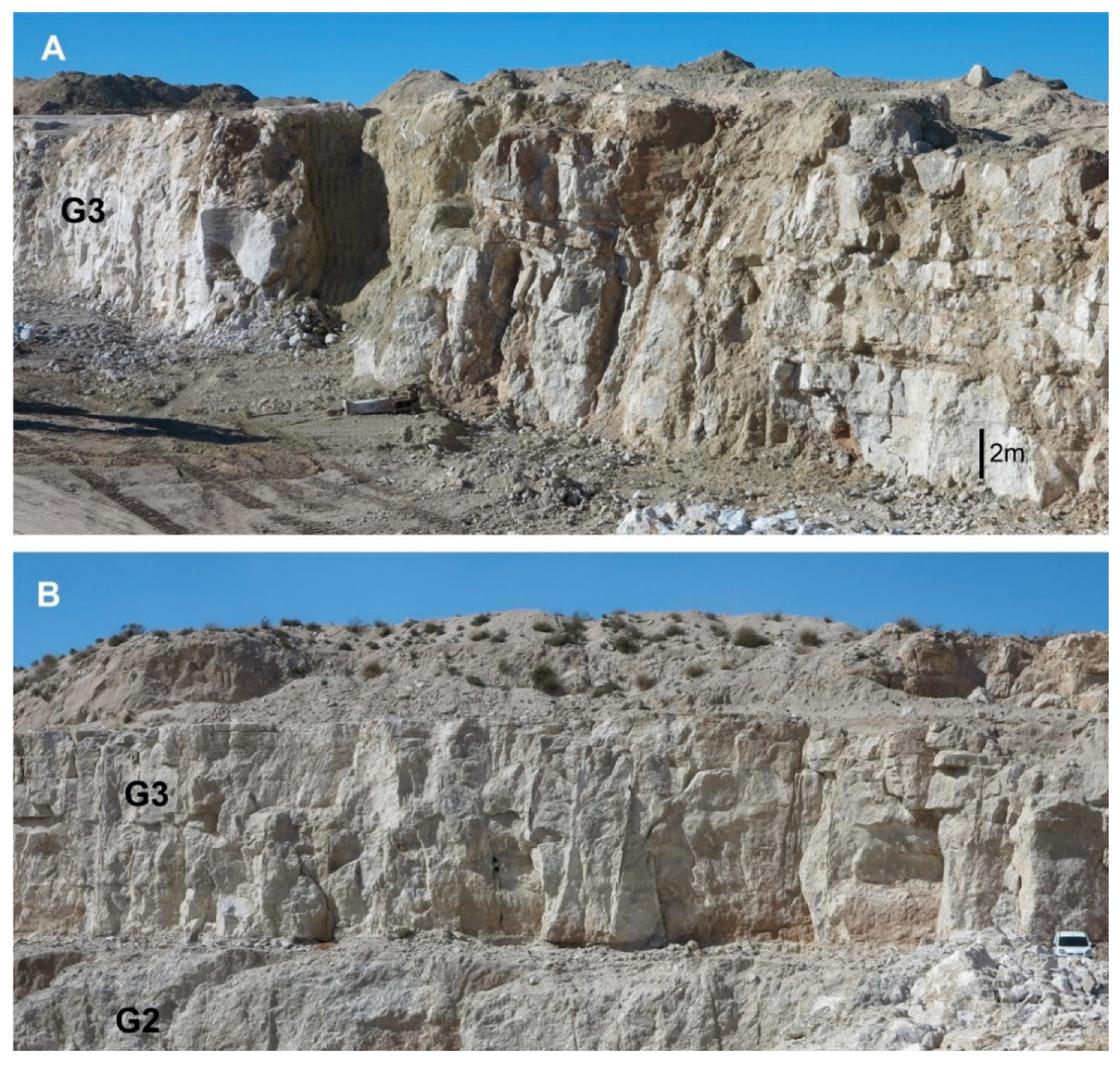
Quarry fronts: (A) view of the quarry, showing a large fracture zone with relatively abundant shaley material, within gypsum bank G3, which could be the similar context in which there is a decrease in resistivity in the subsurface, such as those observed in the ERT profiles performed. (B) Quarry front where there is a continuity of gypsum banks.
Figure 16.
Quarry fronts: (A) view of the quarry, showing a large fracture zone with relatively abundant shaley material, within gypsum bank G3, which could be the similar context in which there is a decrease in resistivity in the subsurface, such as those observed in the ERT profiles performed. (B) Quarry front where there is a continuity of gypsum banks.
Figure 17.
Resistivity data as a function of the saturation conditions from measures on samples with different saturation degrees (modified from Caselle et al., 2019 [
14]).
Figure 17.
Resistivity data as a function of the saturation conditions from measures on samples with different saturation degrees (modified from Caselle et al., 2019 [
14]).
Table 1.
The propagation velocities of seismic waves through different types of geological media (from Tendürüs et al., 2015 [
46] and Earle, 2019 [
47]).
Table 1.
The propagation velocities of seismic waves through different types of geological media (from Tendürüs et al., 2015 [
46] and Earle, 2019 [
47]).
| Medium | S-Wave Velocity (m/s) |
|---|
| Gravel, dry sand | 300–900 |
| Silt and clay | 100–500 |
| Wet sand | 700–800 |
| Gypsum | 600–1500 |
| Sandstone | 1400–2500 |
| Marl | 100–500 |
| Limestone | 2400–3100 |
| Granito | 3000–3700 |
Table 2.
Geoelectrical classification of gypsum rocks (modified after Guinea et al., 2010b, [
51]).
Table 2.
Geoelectrical classification of gypsum rocks (modified after Guinea et al., 2010b, [
51]).
| Lithofacies | Gypsum Content (%) | Resistivity (Ω·m) |
|---|
| Gypsum | 75–100 | 700–1000 |
| Gypsum with lutite | 55–75 | 100–700 |
| Lutites and gypsum-rich lutites | 0–55 | 10–100 |
| Disclaimer/Publisher’s Note: The statements, opinions and data contained in all publications are solely those of the individual author(s) and contributor(s) and not of MDPI and/or the editor(s). MDPI and/or the editor(s) disclaim responsibility for any injury to people or property resulting from any ideas, methods, instructions or products referred to in the content. |
© 2023 by the authors. Licensee MDPI, Basel, Switzerland. This article is an open access article distributed under the terms and conditions of the Creative Commons Attribution (CC BY) license (https://creativecommons.org/licenses/by/4.0/).


