
Response Surface Methodology for Copper Flotation Optimization in Saline Systems

 ,
,  ,
,  ,
, 
Abstract
1. Introduction
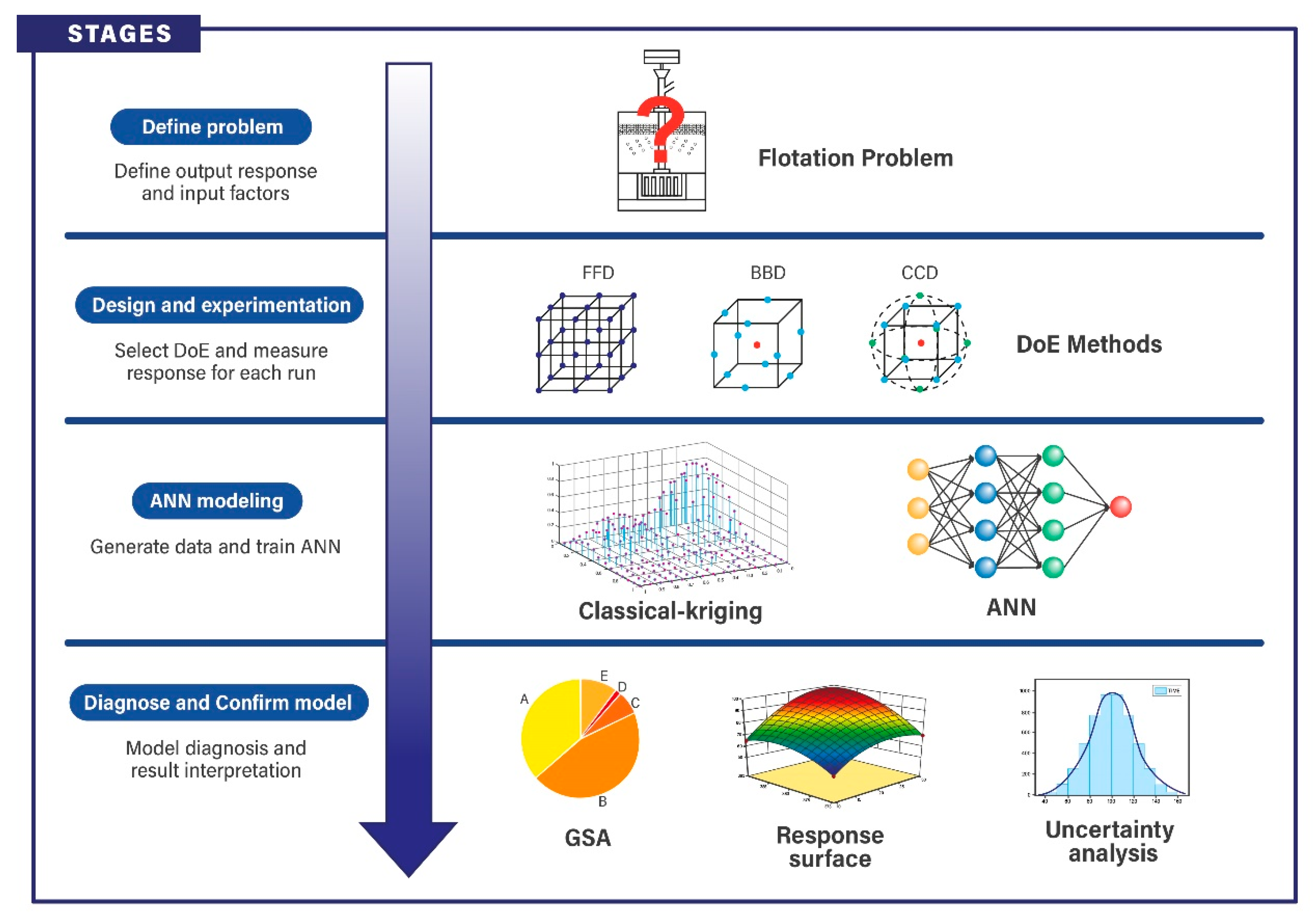
2. Methodology
3. Application of the Methodology
3.1. Description of the Cases and Experimental Setup
3.2. Stage 1: Definition of Input and Output Factors
3.3. Stage 2: Design and Experimentation
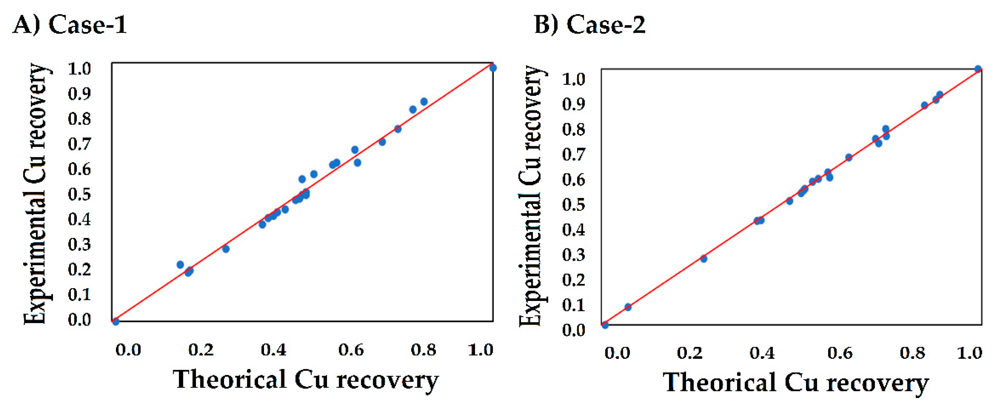
3.4. Stage 3: ANN Fit
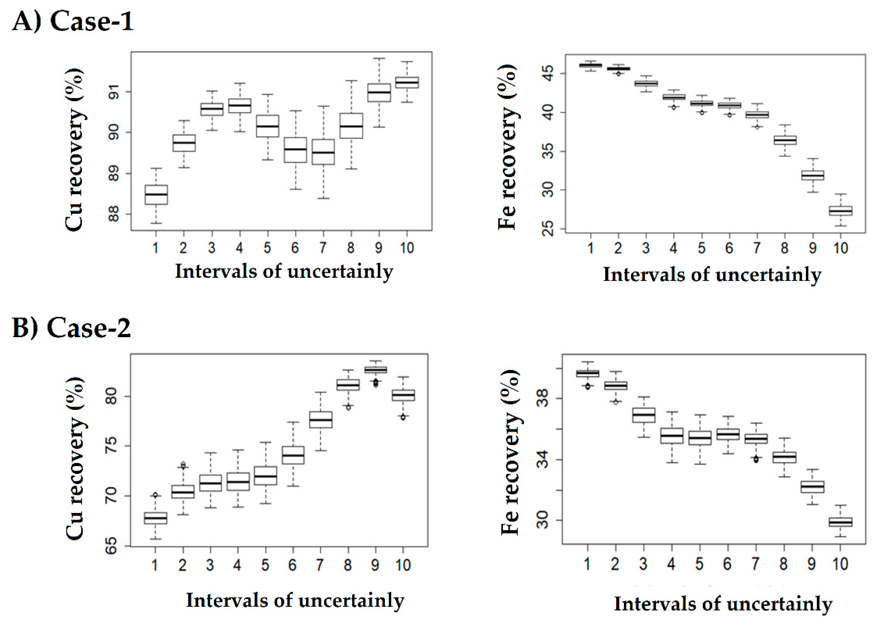
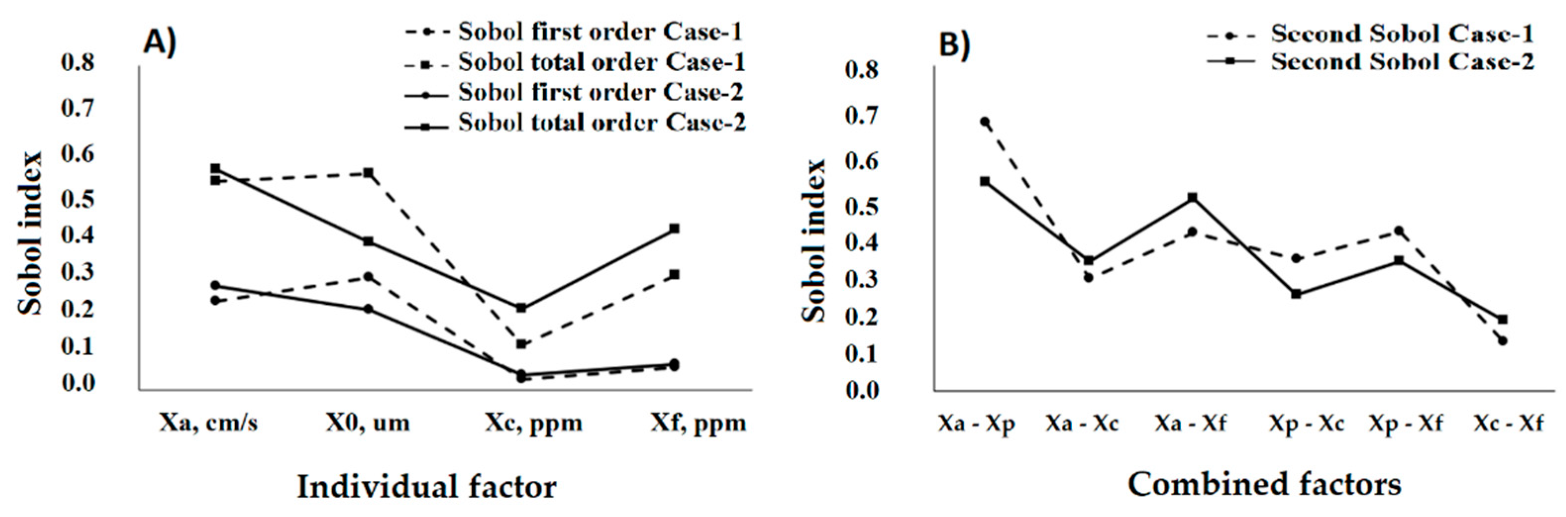
3.5. Stage 4: Diagnose and Confirm Model
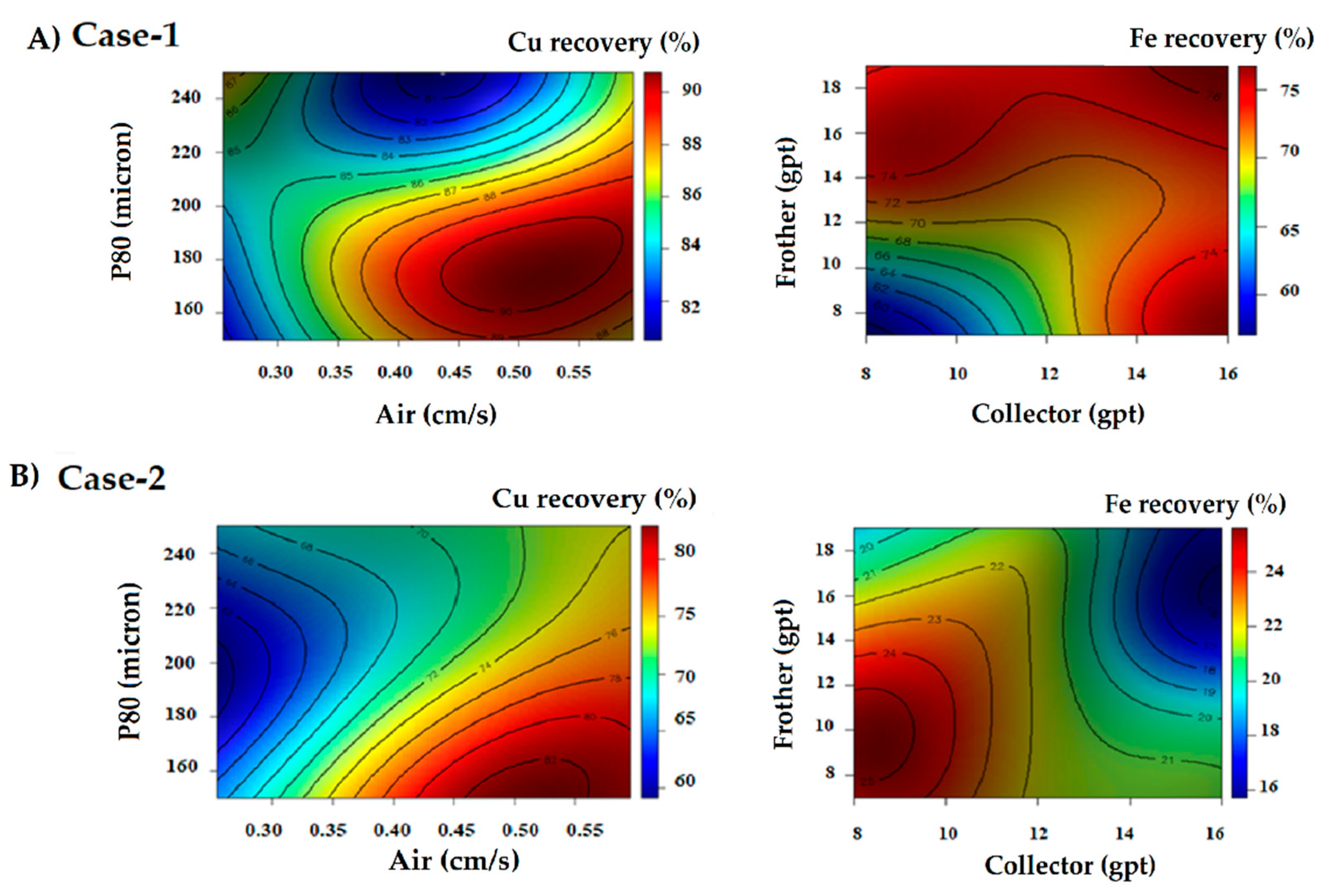
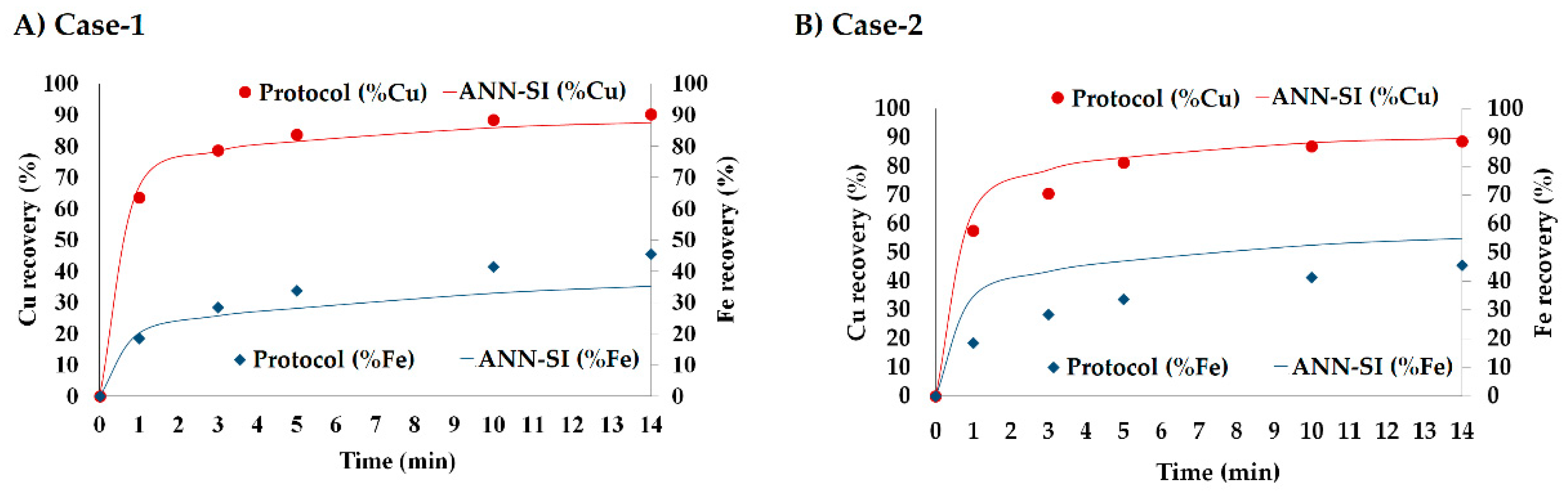
3.6. Model Application
4. Conclusions
Supplementary Materials
Author Contributions
Funding
Data Availability Statement
Acknowledgments
Conflicts of Interest
References
- Gräfe, M.; McFarlane, A.; Klauber, C. Clays and the Minerals Processing Value Chain (MPVC). In Clays in the Minerals Processing Value Chain; Cambridge University Press: Cambridge, UK, 2017; pp. 1–80. [Google Scholar]
- Jeldres, R.I.; Uribe, L.; Cisternas, L.A.; Gutierrez, L.; Leiva, W.H.; Valenzuela, J. The effect of clay minerals on the process of flotation of copper ores—A critical review. Appl. Clay Sci. 2019, 170, 57–69. [Google Scholar] [CrossRef]
- Farrokhpay, S.; Nguyen, A.V.; Thella, J. The influence of water quality on sulfide mineral flotation—A review. In Proceedings of the APCChE 2015 Congress incorporating Chemeca 2015, Melbourne, Australia, 27 September–1 October 2015. [Google Scholar]
- Herrera-León, S.; Lucay, F.A.; Cisternas, L.A.; Kraslawski, A. Applying a multi-objective optimization approach in designing water supply systems for mining industries. The case of Chile. J. Clean. Prod. 2019, 210, 994–1004. [Google Scholar] [CrossRef]
- Li, Y.; Li, W.; Xiao, Q.; He, N.; Ren, Z.; Lartey, C.; Gerson, A.R. The influence of common monovalent and divalent chlorides on chalcopyrite flotation. Minerals 2017, 7, 111. [Google Scholar] [CrossRef]
- Cisternas, L.A.; Gálvez, E.D. The use of seawater in mining. Miner. Process. Extr. Metall. Rev. 2018, 39, 18–33. [Google Scholar] [CrossRef]
- Cruz, C.; Botero, Y.L.; Jeldres, R.I.; Uribe, L.; Cisternas, L.A. Current status of the effect of seawater ions on copper flotation: Difficulties, opportunities, and industrial experience. Miner. Process. Extr. Metall. Rev. 2022, 43, 545–563. [Google Scholar] [CrossRef]
- Aitken, D.; Rivera, D.; Godoy-Faúndez, A.; Holzapfel, E. Water scarcity and the impact of the mining and agricultural sectors in Chile. Sustainability 2016, 8, 128. [Google Scholar] [CrossRef]
- Cisternas, L.A.; Ordóñez, J.I.; Jeldres, R.I.; Serna-Guerrero, R. Toward the implementation of circular economy strategies: An overview of the current situation in mineral processing. Miner. Process. Extr. Metall. Rev. 2021, 43, 775–797. [Google Scholar] [CrossRef]
- Cisternas, L.A.; Lucay, F.A.; Botero, Y.L. Trends in modeling, design, and optimization of multiphase systems in minerals processing. Minerals 2020, 10, 22. [Google Scholar] [CrossRef]
- Box, G.E.P.; Wilson, K.B. On the experimental attainment of optimum conditions. J. R. Stat. Soc. Ser. B Methodol. 1951, 13, 1–38. [Google Scholar] [CrossRef]
- Da, T.; Chen, T.; Ma, Y.; Tong, Z. Application of response surface method in the separation of radioactive material: A review. Radiochim. Acta 2022, 110, 51–66. [Google Scholar] [CrossRef]
- Conde-Hernández, L.A.; Botello-Ojeda, A.G.; Alonso-Calderón, A.A.; Osorio-Lama, M.A.; Bernabé-Loranca, M.B.; Chavez-Bravo, E. Optimization of extraction of essential oils using response surface methodology: A review. J. Essent. Oil Bear. Plants 2021, 24, 937–982. [Google Scholar] [CrossRef]
- Nazlabadi, E.; Niaragh, E.K.; Moghaddam, M.R.A. A systematic and critical review of two decades’ application of response surface methodology in biological wastewater treatment processes. Desalination Water Treat 2021, 228, 92–120. [Google Scholar] [CrossRef]
- Mäkelä, M. Experimental design and response surface methodology in energy applications: A tutorial review. Energy Convers. Manag. 2017, 151, 630–640. [Google Scholar] [CrossRef]
- Tang, Q.; Lau, Y.B.; Hu, S.; Yan, W.; Yang, Y.; Chen, T. Response surface methodology using Gaussian Processes: Towards optimizing the trans-stilbene epoxidation over Co2+–NaX catalysts. Chem. Eng. J. 2010, 156, 423–431. [Google Scholar] [CrossRef]
- Frost, J. How to Interpret R-Squared in Regression Analysis. Available online: https://statisticsbyjim.com/regression/interpret-r-squared-regression/ (accessed on 31 August 2022).
- Torres, M.; Cantú, F. Learning to see: Convolutional neural networks for the analysis of social science data. Political Anal. 2022, 30, 113–131. [Google Scholar] [CrossRef]
- di Franco, G.; Santurro, M. Machine learning, artificial neural networks and social research. Qual. Quant. 2021, 55, 1007–1025. [Google Scholar] [CrossRef]
- Bingöl, D.; Hercan, M.; Elevli, S.; Kılıç, E. Comparison of the results of response surface methodology and artificial neural network for the biosorption of lead using black cumin. Bioresour. Technol. 2012, 112, 111–115. [Google Scholar] [CrossRef] [PubMed]
- Witek-Krowiak, A.; Chojnacka, K.; Podstawczyk, D.; Dawiec, A.; Pokomeda, K. Application of response surface methodology and artificial neural network methods in modelling and optimization of biosorption process. Bioresour. Technol. 2014, 160, 150–160. [Google Scholar] [CrossRef]
- Lucay, F.A.; Sales-Cruz, M.; Gálvez, E.D.; Cisternas, L.A. Modeling of the complex behavior through an improved response surface methodology. Miner. Process. Extr. Metall. Rev. 2021, 42, 285–311. [Google Scholar] [CrossRef]
- Kalyani, V.K.; Pallavika; Chaudhuri, S.; Charan, T.G.; Haldar, D.D.; Kamal, K.P.; Badhe, Y.P.; Tambe, S.S.; Kulkarni, B.D. Study of a laboratory-scale froth flotation process using artificial neural networks. Miner. Processing Extr. Metall. Rev. 2008, 29, 130–142. [Google Scholar] [CrossRef]
- Saltelli, A. Global sensitivity analysis: An introduction. In Sensitivity Analysis of Model Output; Hanson, K.M., Hemez, F.M., Eds.; Los Alamos National Laboratory: Los Alamos, NM, USA, 2005. [Google Scholar]
- Sepúlveda, F.D.; Cisternas, L.A.; Gálvez, E.D. The use of global sensitivity analysis for improving processes: Applications to mineral processing. Comput. Chem. Eng. 2014, 66, 221–232. [Google Scholar] [CrossRef]
- Mellado, M.; Cisternas, L.; Lucay, F.; Gálvez, E.; Sepúlveda, F.D. A posteriori analysis of analytical models for heap leaching using uncertainty and global sensitivity analyses. Minerals 2018, 8, 44. [Google Scholar] [CrossRef]
- Mathe, E.; Cruz, C.; Lucay, F.A.; Gálvez, E.D.; Cisternas, L.A. Development of a grinding model based on flotation performance. Miner. Eng. 2021, 166, 106890. [Google Scholar] [CrossRef]
- Hassanzadeh, A.; Azizi, A.; Kouachi, S.; Karimi, M.; Celik, M.S. Estimation of flotation rate constant and particle-bubble interactions considering key hydrodynamic parameters and their interrelations. Miner. Eng. 2019, 141, 105836. [Google Scholar] [CrossRef]
- Gupta, T.; Ghosh, T.; Akdogan, G.; Bandopadhyay, S. Maximizing REE enrichment by froth flotation of Alaskan coal using Box-Behnken design. Min. Metall. Explor. 2019, 36, 571–578. [Google Scholar] [CrossRef]
- Pattanaik, A.; Rayasam, V. Analysis of reverse cationic iron ore fines flotation using RSM-D-optimal design—An approach towards sustainability. Adv. Powder Technol. 2018, 29, 3404–3414. [Google Scholar] [CrossRef]
- Aksoy, D.O.; Sagol, E. Application of central composite design method to coal flotation: Modelling, optimization and verification. Fuel 2016, 183, 609–616. [Google Scholar] [CrossRef]
- Vieceli, N.; Durão, F.O.; Guimarães, C.; Nogueira, C.A.; Pereira, M.F.C.; Margarido, F. Grade-recovery modelling and optimization of the froth flotation process of a Lepidolite ore. Int. J. Miner. Process. 2016, 157, 184–194. [Google Scholar] [CrossRef]
- Mehrabani, J.V.; Noaparast, M.; Mousavi, S.M.; Dehghan, R.; Ghorbani, A. Process optimization and modelling of Sphalerite flotation from a low-grade Zn-Pb ore using response surface methodology. Sep. Purif. Technol. 2010, 72, 242–249. [Google Scholar] [CrossRef]
- Wang, X.; Bu, X.; Alheshibri, M.; Bilal, M.; Zhou, S.; Ni, C.; Peng, Y.; Xie, G. Effect of scrubbing medium’s particle size distribution and scrubbing time on scrubbing flotation performance and entrainment of Microcrystalline Graphite. Int. J. Coal Prep. Util. 2021, 163, 1932843. [Google Scholar] [CrossRef]
- Lü, C.; Wang, Y.; Qian, P.; Liu, Y.; Fu, G.; Ding, J.; Ye, S.; Chen, Y. Separation of chalcopyrite and pyrite from a copper tailing by ammonium humate. Chin. J. Chem. Eng. 2018, 26, 1814–1821. [Google Scholar] [CrossRef]
- Ahmadi, A.; Rezaei, M.; Sadeghieh, S.M. Interaction effects of flotation reagents for SAG mill reject of copper sulphide ore using response surface methodology. Trans. Nonferrous Met. Soc. China 2021, 31, 792–806. [Google Scholar] [CrossRef]
- Nasirimoghaddam, S.; Mohebbi, A.; Karimi, M.; Reza Yarahmadi, M. Assessment of PH-responsive nanoparticles performance on laboratory column flotation cell applying a real ore feed. Int. J. Min. Sci. Technol. 2020, 30, 197–205. [Google Scholar] [CrossRef]
- Aslan, N.; Fidan, R. Optimization of Pb flotation using statistical technique and quadratic programming. Sep. Purif. Technol. 2008, 62, 160–165. [Google Scholar] [CrossRef]
- Azizi, A.; Masdarian, M.; Hassanzadeh, A.; Bahri, Z.; Niedoba, T.; Surowiak, A. Parametric optimization in rougher flotation performance of a sulfidized mixed copper ore. Minerals 2020, 10, 660. [Google Scholar] [CrossRef]
- Ghodrati, S.; Nakhaei, F.; VandGhorbany, O.; Hekmati, M. Modeling and optimization of chemical reagents to improve copper flotation performance using response surface methodology. Energy Sources Part A Recovery Util. Environ. Eff. 2020, 42, 1633–1648. [Google Scholar] [CrossRef]
- Lopéz, R.; Jordão, H.; Hartmann, R.; Ämmälä, A.; Carvalho, M.T. Study of butyl-amine nanocrystal cellulose in the flotation of complex sulphide ores. Colloids Surf. A Physicochem. Eng. Asp. 2019, 579, 123655. [Google Scholar] [CrossRef]
- Popli, K.; Afacan, A.; Liu, Q.; Prasad, V. Development of online soft sensors and dynamic fundamental model-based process monitoring for complex sulfide ore flotation. Miner. Eng. 2018, 124, 10–27. [Google Scholar] [CrossRef]
- Corpas-Martínez, J.R.; Calero, M.; Pérez, A.; Martín-Lara, M.A.; Amor-Castillo, C.; Navarro-Domínguez, R. Influence of physical and chemical parameters on ultrafine fluorspar froth flotation. Powder Technol. 2020, 373, 26–38. [Google Scholar] [CrossRef]
- Marcin, M.; Sisol, M.; Kudelas, D.; Ďuriška, I.; Holub, T. The differences in evaluation of flotation kinetics of talc ore using statistical analysis and response surface methodology. Minerals 2020, 10, 1003. [Google Scholar] [CrossRef]
- Botero, Y.L.; Serna-Guerrero, R.; López-Valdivieso, A.; Benzaazoua, M.; Cisternas, L.A. New insights related to the flotation of covellite in porphyry ores. Miner. Eng. 2021, 174, 107242. [Google Scholar] [CrossRef]
- Ebrahimi, M.; Azimi, E.; Nasiri Sarvi, M.; Azimi, Y. Hybrid PSO enhanced ANN model and central composite design for modelling and optimization of low-intensity magnetic separation of hematite. Miner. Eng. 2021, 170, 106987. [Google Scholar] [CrossRef]
- Marion, C.; Langlois, R.; Kökkılıç, O.; Zhou, M.; Williams, H.; Awais, M.; Rowson, N.A.; Waters, K.E. A design of experiments investigation into the processing of fine low specific gravity minerals using a laboratory Knelson concentrator. Miner. Eng. 2019, 135, 139–155. [Google Scholar] [CrossRef]
- Cao, M.; Bu, H.; Li, S.; Meng, Q.; Gao, Y.; Ou, L. Impact of differing water hardness on the spodumene flotation. Miner. Eng. 2021, 172, 107159. [Google Scholar] [CrossRef]
- Yadav, A.M.; Singhal, H.; Agarwal, D.; Suman, S. Recovery of energy values from high-ash content washery tailings using waste oils by oil agglomeration. Sep. Sci. Technol. 2022, 57, 1266–1278. [Google Scholar] [CrossRef]
- Wang, S.; Xu, C.; Lei, Z.; Li, J.; Lu, J.; Xiang, Q.; Chen, X.; Hua, Y.; Li, Y. Recycling of zinc oxide dust using ChCl-Urea deep eutectic solvent with nitrilotriacetic acid as complexing agents. Miner. Eng. 2022, 175, 107295. [Google Scholar] [CrossRef]
- Chehreghani, S.; Yari, M.; Zeynali, A.; Akhgar, B.N.; Gharehgheshlagh, H.H.; Pishravian, M. Optimization of chalcopyrite galvanic leaching in the presence of pyrite and silver as catalysts by using response surface methodology (RSM). Rud. Geološko-Naft. Zb. 2021, 36, 37–47. [Google Scholar] [CrossRef]
- Davoodi, P.; Ghoreishi, S.M.; Hedayati, A. Optimization of supercritical extraction of galegine from galega officinalis L.: Neural network modeling and experimental optimization via response surface methodology. Korean J. Chem. Eng. 2017, 34, 854–865. [Google Scholar] [CrossRef]
- Baskar, G.; Renganathan, S. Optimization of L-Asparaginase production by Aspergillus Terreus MTCC 1782 using response surface methodology and artificial neural network-linked genetic algorithm. Asia-Pac. J. Chem. Eng. 2012, 7, 212–220. [Google Scholar] [CrossRef]
- Dil, E.A.; Ghaedi, M.; Ghaedi, A.; Asfaram, A.; Jamshidi, M.; Purkait, M.K. Application of artificial neural network and response surface methodology for the removal of crystal violet by zinc oxide nanorods loaded on activate carbon: Kinetics and equilibrium study. J. Taiwan Inst. Chem. Eng. 2016, 59, 210–220. [Google Scholar] [CrossRef]
- Bashipour, F.; Rahimi, A.; Nouri Khorasani, S.; Naderinik, A. Experimental optimization and modeling of sodium sulfide production from H2S-Rich Off-Gas via response surface methodology and artificial neural network. Oil Gas Sci. Technol. Rev. D’ifp Energ. Nouv. 2017, 72, 9. [Google Scholar] [CrossRef][Green Version]
- Antonopoulou, M.; Papadopoulos, V.; Konstantinou, I. Photocatalytic oxidation of treated municipal wastewaters for the removal of phenolic compounds: Optimization and modeling using response surface methodology (RSM) and Artificial Neural Networks (ANNs). J. Chem. Technol. Biotechnol. 2012, 87, 1385–1395. [Google Scholar] [CrossRef]
- Garg, A.; Jain, S. Process parameter optimization of biodiesel production from algal oil by response surface methodology and artificial neural networks. Fuel 2020, 277, 118–254. [Google Scholar] [CrossRef]
- Ghoreishi, S.M.; Hedayati, A.; Mousavi, S.O. Quercetin extraction from Rosa Damascena Mill via supercritical CO2: Neural network and adaptive neuro fuzzy interface system modeling and response surface optimization. J. Supercrit. Fluids 2016, 112, 57–66. [Google Scholar] [CrossRef]
- Ghoreishi, S.M.; Heidari, E. Extraction of Epigallocatechin-3-Gallate from green tea via supercritical fluid technology: Neural network modeling and response surface optimization. J. Supercrit. Fluids 2013, 74, 128–136. [Google Scholar] [CrossRef]
- İlbay, Z.; Şahin, S.; Büyükkabasakal, K. A novel approach for olive leaf extraction through ultrasound technology: Response surface methodology versus artificial neural networks. Korean J. Chem. Eng. 2014, 31, 1661–1667. [Google Scholar] [CrossRef]
- Kim, B.; Choi, Y.; Choi, J.; Shin, Y.; Lee, S. Effect of surfactant on wetting due to fouling in membrane distillation membrane: Application of response surface methodology (RSM) and artificial neural networks (ANN). Korean J. Chem. Eng. 2020, 37, 1–10. [Google Scholar] [CrossRef]
- Kim, Z.; Shin, Y.; Yu, J.; Kim, G.; Hwang, S. Development of NOx removal process for LNG evaporation system: Comparative assessment between response surface methodology (RSM) and artificial neural network (ANN). J. Ind. Eng. Chem. 2019, 74, 136–147. [Google Scholar] [CrossRef]
- Jafari, S.A.; Jafari, D. Simulation of mercury bioremediation from aqueous solutions using Artificial Neural Network, adaptive neuro-fuzzy inference system, and response surface methodology. Desalination Water Treat. 2015, 55, 1467–1479. [Google Scholar] [CrossRef]
- Halder, G.; Dhawane, S.; Barai, P.K.; Das, A. Optimizing chromium (VI) adsorption onto superheated steam activated granular carbon through response surface methodology and artificial neural network. Environ. Prog. Sustain. Energy 2015, 34, 638–647. [Google Scholar] [CrossRef]
- Karimi, F.; Rafiee, S.; Taheri-Garavand, A.; Karimi, M. Optimization of an air drying process for Artemisia Absinthium leaves using response surface and artificial neural network models. J. Taiwan Inst. Chem. Eng. 2012, 43, 29–39. [Google Scholar] [CrossRef]
- Jawad, J.; Hawari, A.; Zaidi, S. Modeling and sensitivity analysis of the forward osmosis process to predict membrane flux using a novel combination of neural network and response surface methodology techniques. Membranes 2021, 11, 70. [Google Scholar] [CrossRef]
- Kumar, S.; Jain, S.; Kumar, H. Process parameter assessment of biodiesel production from a Jatropha-Algae oil blend by response surface methodology and artificial neural network. Energy Sources Part A Recovery Util. Environ. Eff. 2017, 39, 2119–2125. [Google Scholar] [CrossRef]
- Mohammadi, L.; Zafar, M.N.; Bashir, M.; Sumrra, S.H.; Shafqat, S.S.; Zarei, A.A.; Dahmardeh, H.; Ahmad, I.; Halawa, M.I. Modeling of phenol removal from water by NiFe2O4 nanocomposite using response surface methodology and artificial neural network techniques. J. Environ. Chem. Eng. 2021, 9, 105576. [Google Scholar] [CrossRef]
- Ghanavati Nasab, S.; Semnani, A.; Teimouri, A.; Kahkesh, H.; Momeni Isfahani, T.; Habibollahi, S. Removal of congo red from aqueous solution by hydroxyapatite nanoparticles loaded on zein as an efficient and green adsorbent: Response surface methodology and artificial neural network-genetic algorithm. J. Polym. Environ. 2018, 26, 3677–3697. [Google Scholar] [CrossRef]
- Samuel, O.D.; Okwu, M.O. Comparison of response surface methodology (RSM) and artificial neural network (ANN) in modelling of waste coconut oil ethyl esters production. Energy Sources Part A Recovery Util. Environ. Eff. 2019, 41, 1049–1061. [Google Scholar] [CrossRef]
- Prakash Maran, J.; Priya, B. Modeling of ultrasound assisted intensification of biodiesel production from neem (Azadirachta Indica) oil using response surface methodology and artificial neural network. Fuel 2015, 143, 262–267. [Google Scholar] [CrossRef]
- Onukwuli, O.D.; Nnaji, P.C.; Menkiti, M.C.; Anadebe, V.C.; Oke, E.O.; Ude, C.N.; Ude, C.J.; Okafor, N.A. Dual-purpose optimization of dye-polluted wastewater decontamination using bio-coagulants from multiple processing techniques via neural intelligence algorithm and response surface methodology. J. Taiwan Inst. Chem. Eng. 2021, 125, 372–386. [Google Scholar] [CrossRef]
- Pudza, M.Y.; Abidin, Z.Z.; Rashid, S.A.; Yasin, F.M.; Noor, A.S.M.; Issa, M.A. Sustainable synthesis processes for carbon dots through response surface methodology and artificial neural network. Processes 2019, 7, 704. [Google Scholar] [CrossRef]
- Rajković, K.M.; Avramović, J.M.; Milić, P.S.; Stamenković, O.S.; Veljković, V.B. Optimization of ultrasound-assisted base-catalyzed methanolysis of sunflower oil using Response Surface and Artifical Neural Network methodologies. Chem. Eng. J. 2013, 215–216, 82–89. [Google Scholar] [CrossRef]
- Ranjan, D.; Mishra, D.; Hasan, S.H. Bioadsorption of arsenic: An Artificial Neural Networks and Response Surface methodological approach. Ind. Eng. Chem. Res. 2011, 50, 9852–9863. [Google Scholar] [CrossRef]
- Sabonian, M.; Behnajady, M.A. Artificial neural network modeling of Cr(VI) photocatalytic reduction with TiO2-P25 nanoparticles using the results obtained from response surface methodology optimization. Desalination Water Treat. 2014, 56, 2906–2916. [Google Scholar] [CrossRef]
- Rebollo-Hernanz, M.; Cañas, S.; Taladrid, D.; Segovia, Á.; Bartolomé, B.; Aguilera, Y.; Martín-Cabrejas, M.A. Extraction of phenolic compounds from cocoa shell: Modeling using response surface methodology and artificial neural networks. Sep. Purif. Technol. 2021, 270, 118779. [Google Scholar] [CrossRef]
- Shojaeimehr, T.; Rahimpour, F.; Khadivi, M.A.; Sadeghi, M. A modeling study by response surface methodology (RSM) and artificial neural network (ANN) on Cu2+ adsorption optimization using light expended clay aggregate (LECA). J. Ind. Eng. Chem. 2014, 20, 870–880. [Google Scholar] [CrossRef]
- Yadav, A.M.; Nikkam, S.; Gajbhiye, P.; Tyeb, M.H. Modeling and optimization of coal oil agglomeration using response surface methodology and artificial neural network approaches. Int. J. Miner. Process. 2017, 163, 55–63. [Google Scholar] [CrossRef]
- Vedaraman, N.; Sandhya, K.V.; Charukesh, N.R.B.; Venkatakrishnan, B.; Haribabu, K.; Sridharan, M.R.; Nagarajan, R. Ultrasonic extraction of natural dye from Rubia Cordifolia, optimisation using response surface methodology (RSM) & comparison with artificial neural network (ANN) model and its dyeing properties on different substrates. Chem. Eng. Process. Process Intensif. 2017, 114, 46–54. [Google Scholar] [CrossRef]
- Smith, J.R.; Larson, C. Statistical approaches in surface finishing. Part 3. Design-of-experiments. Trans. IMF 2019, 97, 289–294. [Google Scholar] [CrossRef]
- Vera Candioti, L.; de Zan, M.M.; Cámara, M.S.; Goicoechea, H.C. Experimental design and multiple response optimization. Using the desirability function in analytical methods development. Talanta 2014, 124, 123–138. [Google Scholar] [CrossRef]
- Cam, L.; Yang, G.L. Asymptotics in Statistics; Springer International Publishing: Cham, Switzerland, 2000. [Google Scholar]
- Yaghini, M.; Khoshraftar, M.M.; Fallahi, M. A hybrid algorithm for artificial neural network training. Eng. Appl. Artif. Intell. 2013, 26, 293–301. [Google Scholar] [CrossRef]
- Reid, J.L. The shallow salinity minima of the Pacific ocean. Deep. Sea Res. Oceanogr. Abstr. 1973, 20, 51–68. [Google Scholar] [CrossRef]
- Sobarzo, M.; Figueroa, D. The physical structure of a cold filament in a Chilean upwelling zone (Península de Mejillones, Chile, 23°S). Deep. Sea Res. Part I Oceanogr. Res. Pap. 2001, 48, 2699–2726. [Google Scholar] [CrossRef]
- Martínez, M.; Leyton, Y.; Cisternas, L.; Riquelme, C. Metal removal from acid waters by an endemic microalga from the Atacama Desert for water recovery. Minerals 2018, 8, 378. [Google Scholar] [CrossRef]
- Forbes, E.; Davey, K.J.; Smith, L. Decoupling rehology and slime coatings effect on the natural flotability of chalcopyrite in a clay-rich flotation pulp. Miner. Eng. 2014, 56, 136–144. [Google Scholar] [CrossRef]
- Arancibia-Bravo, M.; Lucay, F.; Sepulveda, F.; Cisternas, L. On the use of Na2SO3 as a pyrite depressant in saline systems and the presence of kaolinite. Physicochem. Probl. Miner. Process. 2021, 57, 168–179. [Google Scholar] [CrossRef]
- Castro, S.; Laskowski, J.S. Froth flotation in saline water. KONA Powder Part. J. 2011, 29, 4–15. [Google Scholar] [CrossRef]
- Laplante, A.R.; Toguri, J.M.; Smith, H.W. The effect of air flow rate on the kinetics of flotation. Part 1: The transfer of material from the slurry to the froth. Int. J. Miner. Process. 1983, 11, 203–219. [Google Scholar] [CrossRef]
- Garcia Zuñiga, H. Sociedad nacional de minería. Bol. Min. De La Soc. Nac. De Min. 1935, 418, 83–86. [Google Scholar]
- Zhang, M.; Xu, N.; Peng, Y. The entrainment of kaolinite particles in copper and gold flotation using fresh water and sea water. Powder Technol. 2015, 286, 431–437. [Google Scholar] [CrossRef]
- Farrokhpay, S. The importance of rheology in mineral flotation: A review. Miner. Eng. 2012, 36–38, 272–278. [Google Scholar] [CrossRef]
- Ekmekçi, Z.; Demirel, H. Effects of galvanic interaction on collectorless flotation behaviour of chalcopyrite and pyrite. Int. J. Miner. Process. 1997, 52, 31–48. [Google Scholar] [CrossRef]
- Azizi, A.; Shafaei, S.Z.; Noaparast, M.; Karamoozian, M. The effect of pH, solid content, water chemistry and ore mineralogy on the galvanic interactions between chalcopyrite and pyrite and steel balls. Front. Chem. Sci. Eng. 2013, 7, 464–471. [Google Scholar] [CrossRef]
- Farrokhpay, S.; Bradshaw, D. Effect of clay minerals on froth stability in mineral flotation: A review. In Proceedings of the 26th International Mineral Processing Congress, IMPC 2012: Innovative Processing for Sustainable Growth—Conference Proceedings, New Delhi, India, 24–28 September 2012; pp. 4601–4611. [Google Scholar]


| DoE | Mineral/Ore type | Input | Output | R-Squared (R2) | Adjusted R-Squared (Adj. R2) | Ref. |
|---|---|---|---|---|---|---|
| CCD | Not defined | Particle size, particle density, bubble size, bubble velocity, and turbulence dissipation rate | Flotation rate constant, particle–bubble encounter efficiency | 0.947 | 0.933 | [28] |
| BBD | REE | Frother dosage, pulp density, and collector dosage | REE recoveries and concentrations | 0.930 | 0.900 | [29] |
| D-optimal design | Iron | Collector dosage, frother dosage, depressant dosage, dispersant dosage, and pH | Grade and recoveries of iron | 0.970 | 0.958 | [30] |
| CCD | Coal | Collector dosage, frother dosage, solid ratio, and airflow rate | Ash contents and combustible recoveries of clean coal | 0.898 | Information not available | [31] |
| CCD | Lepidolite | Collector dosage, flotation time, and pH | Recoveries and grade of lepidolite | 0.96 | Information not available | [32] |
| CCD | Sphalerite | Collector dosage, activator dosage, and pH | Recoveries and grade of sphalerite and lead | 0.879 | 0.794 | [33] |
| BBD | Graphite | Scrubbing medium’s particle size, stirring speed, and solid concentration | Enrichment efficiency of scrubbing flotation (α) | 0.883 | 0.787 | [34] |
| CCD | Chalcopyrite | Pulp pH, depressor dosage, and collector dosage | Copper and sulfur recoveries | 0.990 | 0.981 | [35] |
| BBD | Chalcopyrite | Primary collector dosage, secondary collector dosages, and frother dosages | Grade, recovery, and separation efficiency of copper | 0.955 | 0.900 | [36] |
| CCD | Copper ore | pH and nanoparticle dosage | Grade, recovery, and flotation rate constant | 0.982 | 0.974 | [37] |
| BBD | Lead | Pulp pH, depressor dosage, and collector dosage | Grade and recovery of lead | 0.910 | Information not available | [38] |
| CCD | Copper ore | Collector dosage, depressant dosage, frother dosage, pulp pH, and agitation rate | Copper recoveries | 0.810 | Information not available | [39] |
| CCD | Copper ore | Three collectors and two frother dosages | Copper grade and recovery | 0.940 | 0.910 | [40] |
| Factorial design | Complex sulfide ores | Collector concentration, pH value, and depressant concentration | Grade and recovery of copper and zinc | 0.640 | 0.590 | [41] |
| Factorial design | Lead and zinc | Collector type and the particle size | Grade and recovery of lead and zinc | 0.950 | Information not available | [42] |
| CCD | Fluorite | Aeration flow rate, time of flotation, agitator speed, and pH | Grade and recovery of fluorite | 0.834 | Information not available | [43] |
| Custom design of experiment | Talc ore | Collector, frother, and depressant | Flotation kinetics | 0.9 | Information not available | [44] |
| Factorial design | Covellite | pH and collector concentration | Covellite recovery | 0.9363 | 0.87 | [45] |
| Central composite design | Hematite | Field intensity, drum speed, separating gate position, and particle size | Fe recovery | 0.9447 | 0.9192 | [46] |
| Central composite design | Magnetite | Bowl speed, fluidizing water rate, and solid feed rate | Concentrate grade | 0.93 | 0.87 | [47] |
| Central composite design | LiO2 | Na2CO3, NaOH, CaCl2, and NaOL | Grade of LiO2 using hard-hardness water (HHW) | 0.98 | 0.96 | [48] |
| Box–Behnken design | Coal | Solid concentration, oil dosage, type of oil, and agglomeration time | Ash rejection | 0.9906 | 0.9891 | [49] |
| Central composite design | Oxide zinc | Temperature, time, solid–liquid ratio, and NTA concentration | Zinc extraction | 0.97 | 0.95 | [50] |
| Central composite design | Chalcopyrite | Py/Cp ratio, Ag concentration, potential, and acid concentration | Cu recovery | 0.9744 | Information not available | [51] |
| Sample | Input | Output | DoE | Regression Model (R2) | ANN Type | Hidden Neuron | Regression Model (R2 Adjusted) | Training Algorithm | Ref. |
|---|---|---|---|---|---|---|---|---|---|
| Galegine | Temperature, pressure, flow rate, and extraction time | Experimental yield | CCD | 0.934 | MLP | 6 | 0.9668 | BP | [52] |
| L-asparaginase | L-asparaginase unit, sodium nitrate, L-aspargine, and glucose | L-asparaginase activity | CCD | 0.973 | MLP | - * | 0.997 | Genetic algorithm | [53] |
| Crystal violet | Concentration, pH, adsorbent dosage, and sonication time | Crystal violet removal | CCD | 0.99 | MLP | 20 | 0.999 | BP | [54] |
| Sodium sulfide | Initial NaOH concentration, scrubbing solution temperature, and liquid-to-gas volumetric ratio | Na2S production | CCD | 0.9824 | MLP | 3 | 0.9953 | BP | [55] |
| Wastewater | Initial pH, [H2O2]/[Fe2+] mole ratio, [Fe2+] dosage, and initial COD concentration | Chemical oxygen demand (COD) removal | CCD | 0.9171 and 0.9617 | RBF, MLP | 10 | 0.9810 and 0.9980 | BP and genetic algorithm | [56] |
| Biodiesel | Reaction time, catalyst concentration, and methanol concentration | Biodiesel yield | BBD | 0.9657 | MLP | 9 | 0.999651 | BP | [57] |
| Quercetin | Dynamic time, pressure, temperature, and flow rate of SC-CO2 | Extraction of quercetin | CCD | 0.9317 | MLP | 6 | 0.995 | BP | [58] |
| Green tea | Pressure, temperature, flow rate, and dynamic time | EGCG extraction | CCD | 0.984 | MLP | 6 | 0.997 | BP | [59] |
| Olive leaves | pH, extraction time, temperature, and solid/solvent ratio | Olive leaf extraction | BBD | 0.9315 | MLP | 60 | 0.9746 | BP | [60] |
| Membrane distillation | NaCl, CaSO4, organics, and SDS | Time of wetting occurrence and recovery | CCD | 0.983 and 0.985 | MLP | 6 | 0.999 and 0.999 | BP | [61] |
| Flue gas | Flow rate of the additional oxygen, water temperature, pH, and aqueous concentration of H2O2 | Nox removal in acidic and basic media | CCD | 0.868 and 0.874 | MLP | 3 | 0.9747 and 0.992 | BP | [62] |
| Mercury bioremediation | pH, temperature, and Hg concentration | Mercury removal | CCD | 0.999 | MLP-Fuzzy | 20 | 0.997 and 0.996 | (---) | [63] |
| Aqueous environment | pH, AC dose, contact time, initial concentration, and temperature | Chromium (VI) adsorption | CCD | 0.9886 | MLP | 20 | 0.9911 | BP | [64] |
| Artemisia absinthium leaves | Air temperature, air velocity, and drying time | Air drying | CCD | 0.9423 | MLP | 15 | 0.9997 | BP | [65] |
| Osmosis process | Osmotic pressure difference, feed solution velocity, draw solution velocity, temperature, and DS temperature | Membrane flux | BBD | 0.9408 | MLP | 10 | 0.98036 | BP | [66] |
| Oil yield | Methanol-to-oil ratio, reaction temperature, reaction time, and catalyst amount | Biodiesel production | BBD | 0.9867 | MLP | 10 | 0.9976 | BP | [67] |
| Wastewater | NFC amount, contact time, pH, and phenol concentration | Phenol removal | CCD | 0.961 | MLP | 6 | 0.9934 | BP | [68] |
| Wastewater | pH, contact time, temperature, CR concentration, and adsorbent dosage | Congo red removal | CCD | 0.9954 | MLP | 9 | 0.9983 | BP | [69] |
| Biodiesel | Reaction temperature, ethanol, and catalyst amount | Coconut oil ethyl ester (CNOEE) yield | CCD | 0.9564 | MLP | 10 | 0.998 | BP | [70] |
| Neem (azadirachta indica) oil | Methanol-to-oil molar ratio, catalyst concentration, reaction temperature, and reaction time | FAME conversion | CCD | 0.919 | MLP | 9 | 0.999 | BP | [71] |
| Wastewater | Dosage, pH, and stirring time | CTSP removal | BBD | 0.9871 | MLP | 10 | 0.999 | BP | [72] |
| Carbon dots | Temperature, dosage, time, and W/Ace/NaOH ratio | Fluorescent CDs synthesis | CCD | 0.9563 | MLP | 20 | 0.944 | BP | [73] |
| Biodiesel | Reaction temperature, ethanol-to-oil molar ratio, catalyst loading, and reaction time | FAME yield | 34 full factorial | 0.803 | MLP | 20 | 0.947 | BP | [74] |
| Wastewater | pH, temperature, and b dose | Bioadsorption of arsenic | CCD | 0.9843 | MLP | - | 0.9952 | BP | [75] |
| Wastewater | Initial concentration of Cr(VI), varying dosages of photocatalyst, different irradiation times, and pHs | Cr(VI) photocatalytic reduction | CCD | 0.9812 | MLP | 4 | 0.9858 | BP | [76] |
| Cocoa shell | Temperature, time, acidity, and ratio | Extraction of phenolic compounds (TPA) | BBD | 0.9256 | MLP | 10 | 0.98 | BFGS, quasi-Newton backpropagation, gradient descent | [77] |
| Wastewater | pH, temperature, initial concentration, and adsorbent dosage | Cu2+ adsorption optimization | CCF | 0.941 | MLP | 4 | 0.962 | BP | [78] |
| Coal | Solid concentration, oil dosage, and agglomeration time | % ash rejection | BBD | 0.9956 | MLP | 3 | 0.9965 | Levenberg–Marquardt, Bayesian regularization, gradient descent with momentum, gradient descent | [79] |
| Rubia cordifolia | Ultrasonic frequency, solid-to-liquid ratio, and extraction time | Natural dye extraction | CCD | 0.9805 | MLP | 10 | 0.9853 | BP | [80] |
| Wastewater | pH, turbidity, BOD, and COD | COD removal (%) | BBD | 0.9754 | MLP | 10 | 0.9924 | BP |
| Sample | Cu | Fe | Mo |
|---|---|---|---|
| Case 1 | 0.28 | 4.81 | 0.0085 |
| Case 2 | 0.27 | 3.95 | 0.0087 |
| Minerals | Case 1 | Case 2 | Minerals | Case 1 | Case 2 |
|---|---|---|---|---|---|
| Chalcocite/digenite | 0.03 | 0.05 | Siderite | 0.01 | 0.01 |
| Covellite | 0 | 0.01 | Calcite/dolomite | 0.42 | 0.59 |
| Chalcopyrite | 0.63 | 0.46 | Apatite | 0.56 | 0.48 |
| Bornite | 0.01 | 0.02 | Quartz | 21.94 | 30 |
| Tetrahedrite group | 0 | 0.01 | Orthoclase (K-feldspars) | 2.68 | 4.12 |
| Other Cu minerals | 0.01 | 0.01 | Plagioclase (Ca, Na-feldspars) | 31.46 | 17.66 |
| Cu-bearing phyllosilicates | 1.3 | 1.27 | Kaolinite group | 1.92 | 1.07 |
| Cu-bearing Fe Oxy/hydroxides | 0 | 0.01 | Muscovite/sericite | 1.42 | 3.12 |
| Cu-bearing wad | 0.07 | 0.17 | Illite | 0.35 | 0.87 |
| Pyrite | 2.58 | 4.48 | Smectite group (montmorillonite, nontronite) | 0.34 | 0.35 |
| Molybdenite | 0.04 | 0.02 | Pyrophyllite | 0.21 | 0.25 |
| Sphalerite | 0.01 | 0.02 | Chlorite group | 15.39 | 21.82 |
| Magnetite | 0.88 | 0.44 | Biotite/phlogopite | 11.21 | 4.8.0 |
| Hematite | 0.74 | 0.47 | Hornblende | 0.11 | 0.15 |
| Goethite | 0.03 | 0.03 | Tourmaline group | 0.48 | 0.26 |
| Other Fe Oxy/hydroxides | 0.1 | 0.08 | Titanite | 0.14 | 0.09 |
| Gypsum/anhydrite | 3.97 | 5.6 | Rutile | 0.4 | 0.51 |
| Jarosite | 0.06 | 0.14 | Ilmenite | 0.24 | 0.19 |
| Alunite | 0.08 | 0.21 | Other gangue | 0.17 | 0.18 |
| Total | 100 | 100 |
| Parameter | Value | Parameter | Value |
|---|---|---|---|
| Mg2+ (mg L−1) | 1310 ± 38 | NO3− (mg L−1) | 3.62 ± 0.38 |
| Na+ (mg L−1) | 11,138 ± 12 | HCO3− (mg L−1) | 143 ± 5 |
| K+ (mg L−1) | 401 ± 4 | SO42− (mg L−1) | 2791 ± 18 |
| Ca2+ (mg L−1) | 415 ± 26 | Conductivity (mS cm−1) | 53.4 ± 1.2 |
| Cl− (mg L−1) | 19,867 ± 24 | pH | 7.98 ± 0.08 |
| Factors | Code Factor Level | ||
|---|---|---|---|
| Low | Center | High | |
| −1 | 0 | 1 | |
| : Air, cm/s | 0.34 | 0.51 | 0.68 |
| : P80, µm | 150 | 210 | 250 |
| : Collector, gpt | 8 | 12 | 16 |
| : Frother, gpt | 7 | 13 | 19 |
| Run | Input Factors | Output Factors | ||||||
|---|---|---|---|---|---|---|---|---|
| Case 1 | Case 2 | |||||||
| 15 | 0 | 0 | −1 | −1 | 87.8 | 42.1 | 57.1 | 37.0 |
| 11 | −1 | −1 | 0 | 0 | 84.8 | 43.6 | 69.7 | 43.7 |
| 4 | 0 | 0 | 0 | 0 | 84.8 | 38.3 | 66.6 | 43.3 |
| 9 | 0 | 1 | 0 | −1 | 84.7 | 29.4 | 66.6 | 43.6 |
| 8 | −1 | 0 | 0 | 1 | 84.9 | 39.1 | 60.9 | 41.9 |
| 7 | 1 | 0 | 0 | 1 | 84.8 | 41.6 | 71.5 | 40.8 |
| 23 | 1 | 0 | 0 | −1 | 84.7 | 25.0 | 78.1 | 46.4 |
| 21 | 0 | 1 | 1 | 0 | 84.7 | 29.8 | 77.6 | 43.8 |
| 6 | 1 | 0 | −1 | 0 | 84.7 | 39.2 | 77.6 | 44.4 |
| 2 | 1 | 0 | 1 | 0 | 87.9 | 42.1 | 80.9 | 45.3 |
| 3 | −1 | 0 | −1 | 0 | 81.9 | 35.0 | 79.2 | 34.3 |
| 16 | −1 | 0 | 1 | 0 | 84.9 | 25.3 | 76.3 | 37.5 |
| 17 | 0 | −1 | −1 | 0 | 87.9 | 42.8 | 86.8 | 47.9 |
| 5 | 0 | 0 | 1 | −1 | 87.9 | 33.1 | 82.6 | 37.3 |
| 18 | 0 | 1 | −1 | 0 | 81.6 | 40.1 | 80.6 | 39.4 |
| 12 | 0 | 1 | 0 | 1 | 84.8 | 37.9 | 83.2 | 43.0 |
| 24 | −1 | 1 | 0 | 0 | 84.9 | 37.3 | 76.3 | 37.9 |
| 1 | 0 | −1 | 0 | −1 | 84.9 | 41.0 | 86.5 | 46.4 |
| 19 | 1 | 1 | 0 | 0 | 87.8 | 27.4 | 83.5 | 38.9 |
| 26 | 0 | −1 | 1 | 0 | 88.0 | 27.1 | 86.6 | 43.6 |
| 27 | 0 | 0 | 0 | 0 | 84.8 | 40.7 | 80.2 | 41.5 |
| 14 | 1 | −1 | 0 | 0 | 88.0 | 37.2 | 89.8 | 49.4 |
| 13 | −1 | 0 | 0 | −1 | 84.8 | 41.7 | 79.6 | 37.8 |
| 10 | 0 | 0 | 0 | 0 | 87.8 | 39.6 | 83.3 | 44.7 |
| 25 | 0 | −1 | 0 | 1 | 88.0 | 37.3 | 86.4 | 45.0 |
| 20 | 0 | 0 | 1 | 1 | 87.9 | 25.4 | 86.1 | 41.6 |
| 22 | 0 | 0 | −1 | 1 | 87.9 | 32.1 | 82.8 | 37.8 |
| Case | Input Factors | |||
|---|---|---|---|---|
| cm/s | µm | gpt | gpt | |
| Case 1 | 0.54 | 190.7 | 10.5 | 18.9 |
| Case 2 | 0.52 | 150.1 | 11.0 | 14.2 |
| Case | Kinetics Parameters | |||||
|---|---|---|---|---|---|---|
| Cu | Fe | |||||
| % | 1/min | Standard Error | % | 1/min | Standard Error | |
| Case 1 | 87.5 | 1.4 | 100.0 | 35.3 | 0.5 | 63.8 |
| Case 2 | 89.8 | 1.2 | 119.1 | 54.9 | 0.8 | 114.4 |
Publisher’s Note: MDPI stays neutral with regard to jurisdictional claims in published maps and institutional affiliations. |
© 2022 by the authors. Licensee MDPI, Basel, Switzerland. This article is an open access article distributed under the terms and conditions of the Creative Commons Attribution (CC BY) license (https://creativecommons.org/licenses/by/4.0/).
Share and Cite
Arancibia-Bravo, M.P.; Lucay, F.A.; Sepúlveda, F.D.; Cortés, L.; Cisternas, L.A. Response Surface Methodology for Copper Flotation Optimization in Saline Systems. Minerals 2022, 12, 1131. https://doi.org/10.3390/min12091131
Arancibia-Bravo MP, Lucay FA, Sepúlveda FD, Cortés L, Cisternas LA. Response Surface Methodology for Copper Flotation Optimization in Saline Systems. Minerals. 2022; 12(9):1131. https://doi.org/10.3390/min12091131
Chicago/Turabian StyleArancibia-Bravo, María P., Freddy A. Lucay, Felipe D. Sepúlveda, Lorena Cortés, and Luís A. Cisternas. 2022. "Response Surface Methodology for Copper Flotation Optimization in Saline Systems" Minerals 12, no. 9: 1131. https://doi.org/10.3390/min12091131
APA StyleArancibia-Bravo, M. P., Lucay, F. A., Sepúlveda, F. D., Cortés, L., & Cisternas, L. A. (2022). Response Surface Methodology for Copper Flotation Optimization in Saline Systems. Minerals, 12(9), 1131. https://doi.org/10.3390/min12091131