Article

Sulfur Isotopic Composition of Gypsum from Paleocene, Northwest China: Implications for the Evolution of Eastern Paratethys Seawater

1
Institute of Geology, Chinese Academy of Geological Sciences, Beijing 100037, China
2
MNR Key Laboratory of Metallogeny and Mineral Assessment, Institute of Mineral Resources, Chinese Academy of Geological Sciences, Beijing 100037, China
*
Authors to whom correspondence should be addressed.
Minerals 2022, 12(8), 1031; https://doi.org/10.3390/min12081031
Submission received: 9 July 2022 / Revised: 13 August 2022 / Accepted: 13 August 2022 / Published: 16 August 2022
(This article belongs to the Special Issue Mineralogy, Petrology and Geochemistry of Evaporites, Volume II)

Abstract

:
The sulfate isotope record of marine sedimentary sulfate through time has been used successfully to determine global variations in the composition of seawater sulfate. The variations in the sulfur isotope composition of marine sulfate reflect changes in the global sulfur cycle and are also closely related to changes in the atmospheric oxygen cycles. However, data for the Paleocene are very sparse and the stratigraphic evolution of the sulfur isotope composition of seawater is poorly constrained due to the small number of samples analyzed. The Yarkand Basin, as a northeastern part of the eastern Paratethys ocean with the trumpet-shaped bay, in which a suite of evaporitic sequences named the Aertashen Formation was continuously developed in the Paleocene and was principally composed of massive gypsum interbedded fragmental rocks. The values of sulfur isotopic composition are from 12.2‰ to 20.6‰ (δ34 SCDT or δ34 SVCDT) and the mean is 17.7‰ in 97 gypsum samples in the basin. Three gradually increasing trends of sulfur isotopic curves reflect that enrichment of δ34 S occurred in seawater sulfate, and indicate oxidation of seawater sulfide. These may hint to at least three oxidation events or the bacterial reduction of seawater sulfide that occurred in the Paleocene, and that three oxygen-enriched events or the biological sulfur cycle might exist in this epoch. The sulfur isotopic composition (δ34 SCDT or δ34 SVCDT) in the seawater of the northeastern part of the eastern Paratethys ocean was about 15.0‰ to 20.6‰, and averaged 17.9‰ in the Paleocene. Combined with the previous global sulfur isotopic composition of seawater, the final range of global sulfur isotopic composition of seawater might be from 15.0‰ to 21.0‰, with 17.9‰–18.3‰ the average in the Paleocene, so the variations in the sulfur isotope composition of Paleocene seawater sulfate are reconstructed and supplemented.

1. Introduction

The concentration of sulfate in the ocean reflects the balance between the terrestrial weathering of sulfur-bearing minerals and the burial of sulfur as evaporites and sedimentary sulfides in the oceans [1,2]. The isotope record of marine sedimentary sulfate through time has been used successfully to determine global variations in the composition of seawater sulfate [3]. The variations in the sulfur isotopic composition of marine sulfate reflect changes in the global sulfur cycle and are also closely related to changes in atmospheric oxygen cycles [4,5,6]. A global sulfur isotope record for the Phanerozoic based on the analysis of sulfate minerals in evaporites was first reconstructed by Holser and Kaplan [7], Holser [8], and Claypool [9], and some researchers have given good supplementary datum later [3,5,10,11,12]. However, data for the Paleocene are very sparse and the stratigraphic evolution of the sulfur isotopic composition of seawater is poorly constrained due to the small number of samples analyzed. One of the main problems with evaporite-based reconstructions of the δ34 S of marine sulfate is the discontinuous occurrence of evaporites deposits, due to an unfavorable depositional environment and lack of diagnostic fossils.
Evaporites are closely related to geotectonic activity and marine transgressive-regressive cycles [13,14,15,16]. Massive evaporites sequences generally occur at the end of global geotectonic cycles, which are usually associated with global marine regression [17]. Multiple marine transgressive-regressive cycles and evaporites sequences have been identified in the northwestern Tarim Basin (also named the Yarkand Basin) of China in the Late Cretaceous–Paleogene [18,19,20,21], as a northeastern part of the eastern Paratethys ocean with the trumpet-shaped bay in which lagoon deposits occurred and recorded the evolutionary history of sulfur isotopic composition on the eastern Paratethys seawater.
In the Paleocene, a suite of evaporitic depositional sequences named the Aertashen Formation continuously developed in the Yarkand Basin, principally composed of massive gypsum-interbedded thin fragmental rocks in an intermittent marine regression environment (Figure 1a). The accumulated thickness of some gypsum outcrops ranges from several to hundreds of meters. The evaporites of the Aertashen Formation spread almost across the whole Yarkand basin, with the three main gypsum field outcrops spread across this area as well. These outcrops are named Dashankou (hereinafter DSK), Aertashen (hereinafter AET), and Keliyang (hereinafter KLY) (Figure 1a and Figure 2a–d), respectively. The Aertashen Formation covers the area from the South Tianshan and West Kunlun piedmonts in the west, to the Hotan area in the south, and from the Markit slope in the east to the vicinity of Minc1 in the southeast, with additional evidence found in boreholes Minc1 and Mac1 (Figure 1a). It is viable to reconstruct the variations in the sulfur isotopic composition of marine sulfate in Paleocene seawater, and to provide a good supplement to the global sulfur isotope record.

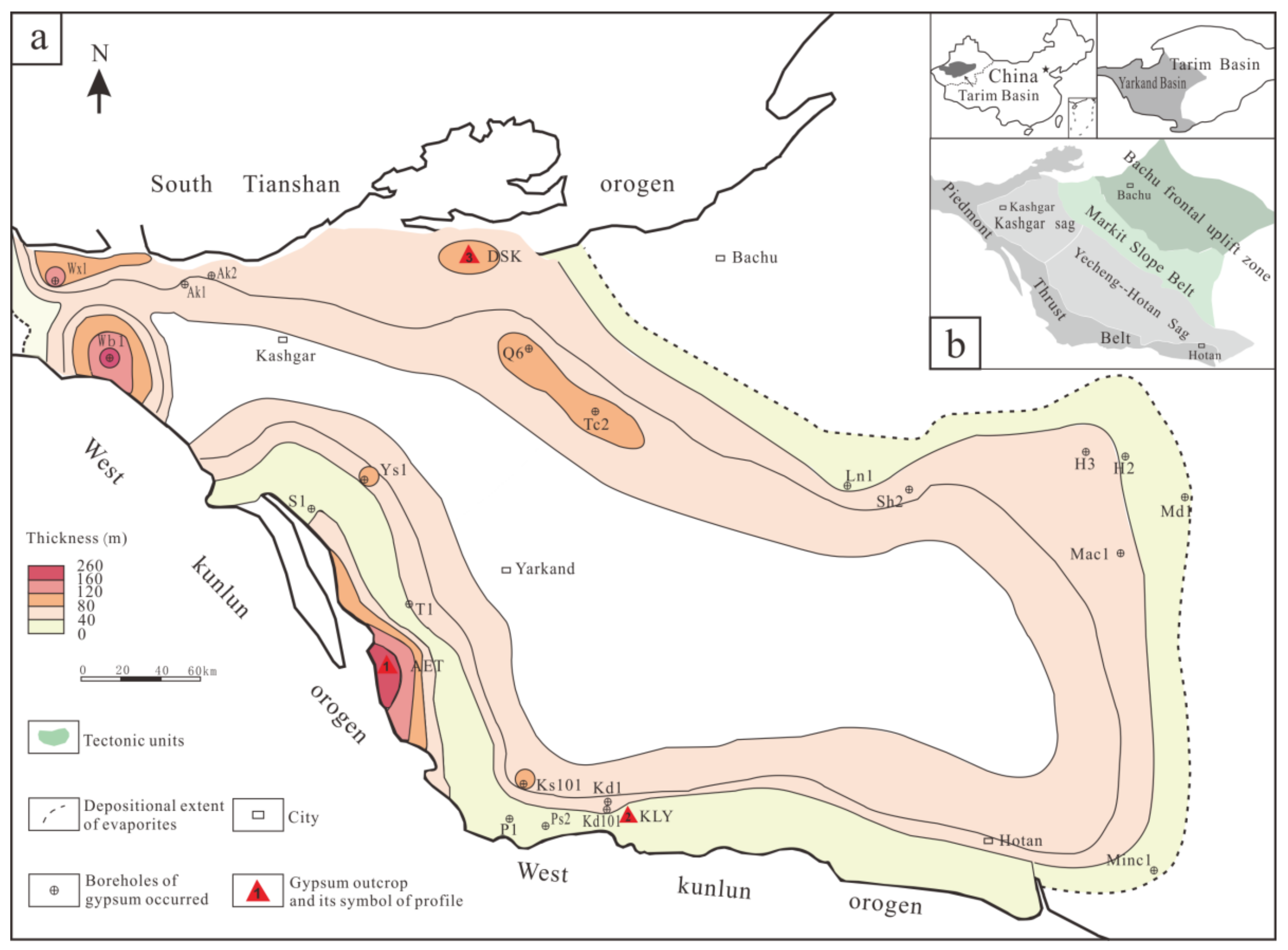
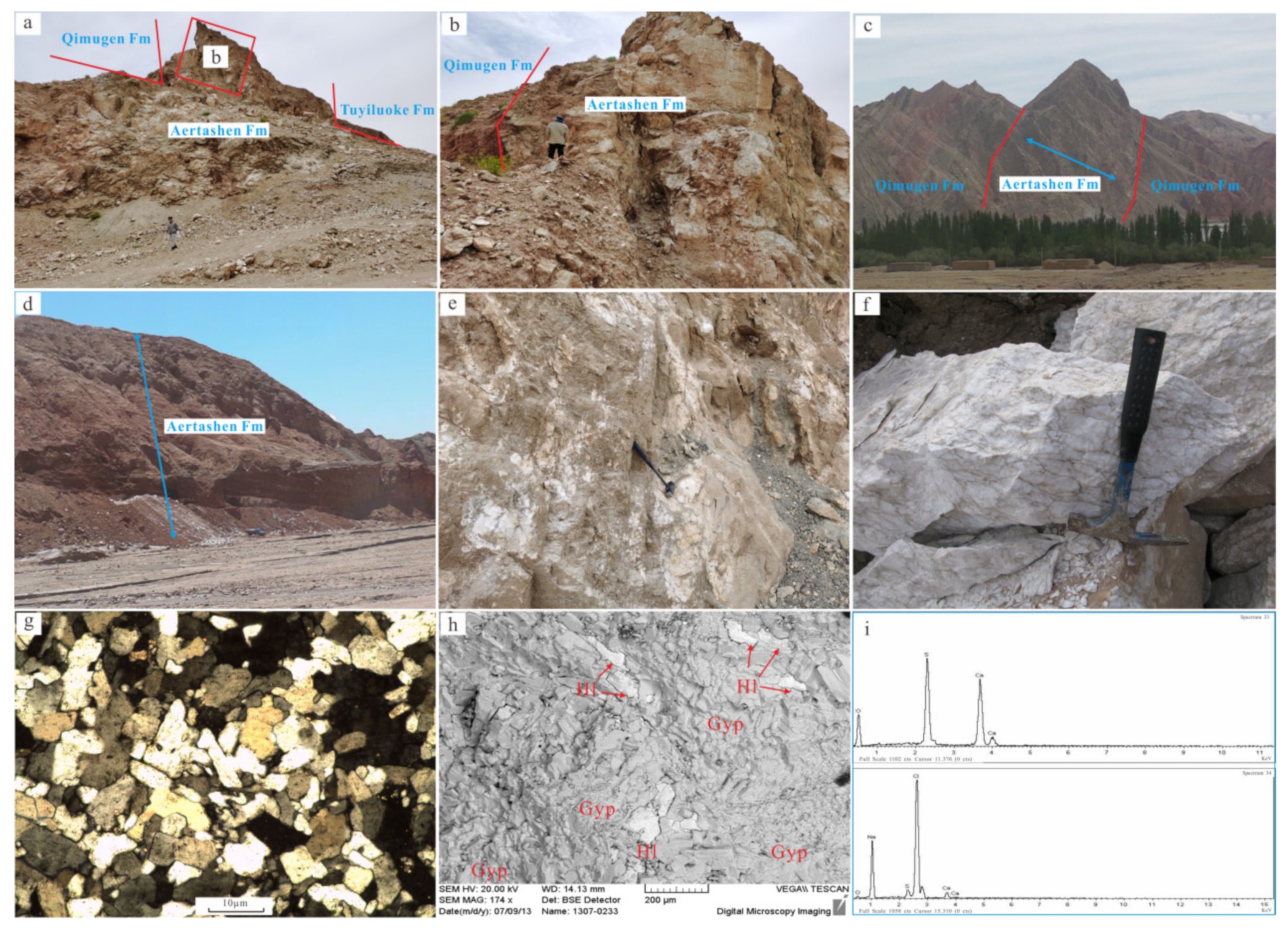
2. Geological Setting

The Yarkand Basin is located in the western Tarim Basin, as a foreland basin that developed from the Pre-Sinian basement and has been reformed multiple times by tectonic superimpositions [22]. From the West Kunlun piedmont to the interior of the basin, it is characterized by a piedmont thrust belt and central sag, which divided the Kashgar and Yecheng-Hotan sags, the Markit slope belt, and the Bachu frontal uplift zone sequentially [23,24] (Figure 1b). The Yarkand Basin was an inherited graben basin in the early Cretaceous, but during the late Cretaceous–Paleogene it had begun to develop into a foreland basin, with its depositional center distributed along the West Kunlun to South Tianshan piedmonts [25]. Since the Cenozoic era, the basin has subsided and deformed, developing several subsiding centers and very thick depositional cap rocks due to the collision of the Indian and Eurasian plates [26]. In the Neogene, the maximum depositional thickness of this basin was located in the Yecheng-Hotan sag, but its depositional center has already migrated along the northwest line to the Kashgar sag since the Quaternary [27].
In the early Cretaceous, the Yarkand Basin was a strip-shaped graben basin with NW-SE orientation located at the West Kunlun piedmont with the largest subsiding center [28]. Sedimentation into the basin was controlled by the provenances of the South Tianshan and West Kunlun orogens. Sediments were distributed along the long strip-shaped West Kunlun piedmont, with thickness gradually decreasing from SW to NE orientation, developing into an alluvial fan, fan delta, and shore-neritic sub-facies [29]. In the late Cretaceous, a braided river delta, supratidal evaporated sand–mud flat, and a carbonate platform developed sequentially [30], and a salt–gypsum flat was deposited in the basin. In the Paleocene–early Eocene, this basin developed into a semi-closed estuarine and lagoon environment. Affected by terrigenous debris and subtropical dry climate [31,32], clastic rocks, in addition to evaporites and carbonates, were developed during this period [33,34,35]. The main evaporative sequences are the Tuyiluoke and Aertashen Formations; the former usually belongs to the Later Maastrichtian stage [36,37,38] and the latter to the Paleocene [33,36,37,38], but the former is smaller than the latter in extent or scale. The Tuyiluoke Formation, mainly composed of sandstones, mudstones, gypsiferous mudstone interbedded with poor gypsum, and small lenticular-shaped halite deposits in the late Cretaceous, is intermittent occurrence in the basin.

3. Methods

Thirty-eight samples were collected from the Keliyang gypsum outcrops (Figure 1a and Figure 2a,b). From bottom to top, the continuous stratigraphic units of the outcrops can be divided into the upper Cretaceous Tuyiluoke Formation, the Palaeogene Aertashen Formation, and Qimugen Formation (Figure 2a–c). The total vertical thickness of the KLY profile is about 28.4 m, from bottom to top the sample interval is 0.5 m with the first five, and about 0.8 m with the later 33 samples for the fine sample. Moreover, fifty-nine data of sulfur isotopic composition of gypsum are cited to make a contrastive analysis of the fluctuation of sulfate isotopic composition from Cao et al. [39,40]. The datum of the sulfur isotopic composition of the additional 59 gypsum samples in the basin comes from the AET and DSK profiles and Wx1, Wb1, Mac1, Minc1, and Tc2 boreholes (Table 1, Figure 1a). All the samples are from the marine depositional gypsum of evaporites outcrops of the Aertashen Formation in the Yarkand Basin, and the integrity of the gypsum record is confirmed to ensure the pristine nature of the record and lack of postdepositional alteration. The geological phenomena of dissolved sulfate (such as gypsum) or biological sulfur cycle have not been observed so far in the field or SEM/flake image.
All of the samples were analyzed at the Analysis and Testing Center of Beijing Institute of Geology of Nuclear Industry. An appropriate amount of sulfate sample containing sulfur about 15 mg was taken to extract barium sulfate by a semi-melting method using the mixed solvent of sodium carbonate and zinc oxide. Mix barium sulfate, vanadium pentoxide, and quartz sand in a weight ratio of 1:3:3.5. In the near vacuum state (2.0 × 10⁻² Pa) was heated and oxidized at 980 ℃ to generate sulfur dioxide gas, which was gathered by freezing method and then analyzed by Delta V Plus gas isotope mass spectrometry for sulfur isotope composition. The calculated results were recorded by δ34 SV-CDT with CDT as standard; the analytical accuracy is better than ±0.2‰. The reference standard of sulfide is GBW-04414 and GBW-04415 silver sulfide, and its δ34 S is −0.07 ± 0.13‰ and 22.15 ± 0.14‰, respectively.

4. Results

The results of the sulfur isotopic composition of samples collected from KLY profile are presented in Table 2. The 38 values of δ34 SVCDT range from 13.8‰ to 19.0‰, and the mean is 17.6‰. If one discounts samples KLY-G35 to G38 (located in the upper profile and the values altered sharply), the values range from 16.2‰ (sample KLY-G1) to 19.0‰ (sample KLY-G15), and the mean is 17.9‰. The values of the δ34 SVCDT range from 16.2, increase to 19.0 and then decline to 17.7 (sample KLY-G25), abruptly increase to 18.3 (sample KLY-G26), and then decline to 16.5, ultimately persistently declining to 13.8 (sample KLY-G38) although momentarily increasing to 15.8 (sample KLY-G37).

5. Discussion

5.1. Sulfur Isotopic Composition of Gypsum in the Yarkand Basin in the Paleocene

Due to the great thickness of the overlying Neogene and Quaternary strata (near 7900 m) and the few boreholes in the interior of the Yarkand basin, it is difficult to collect borehole data in the Kashgar and Yecheng-Hotan sags (Figure 1b). Although there are some boreholes, none of them reached the evaporitic depositional sequences of the Aertashen Formation. Therefore, the boreholes of gypsum observed are mainly located in the periphery areas of this basin, including the West Kunlun and South Tianshan piedmonts and the Markit slope, totaling 21 boreholes (Figure 1a). Therefore, some data of the sulfur isotope composition of gypsum in the basin are selected from the AET (15 samples) and DSK (26 samples) profiles and Wx1 (four samples), Wb1 (three samples), Mac1 (three samples), Minc1 (five samples) and Tc2 (three samples) boreholes (Figure 1a, Table 1), and are used to analyze the history of sulfur isotopic composition of the eastern Paratethys in the Paleocene. The Aertashen Formation gypsum is mainly composed of gypsum (Figure 2e,f), such as the KLY profile (Figure 2g); small quantities of halite (Figure 2h,i) in the gypsum by flake analysis, scanning electron microscope (SEM) and energy dispersive X-ray spectrometer (EDS).
The sulfur isotopic fractionation is weak but significant (only 0.2‰ of instrumental error) in the precipitation process of gypsum. The sulfate in modern evaporitic basins and bays where evaporites are developed have almost the same sulfur isotopic composition [7,41]. The sulfur isotopic composition of modern ocean water and sea water replenished by non-continental rivers is similar to that of the ocean (such as the Red Sea), and the value of δ34 SCDT generally ranges from 18‰ to 25‰ [42]. The ratio of sulfur isotope δ34 SCDT in the ocean near estuaries is reduced, and the value of δ34 SCDT is 8.6‰ to 7.7‰, respectively [43,44]. The sulfur isotopic variation of ancient seawater evaporites is sometimes no more than ±2‰ (δ34 SCDT) in the same basin and geological stage (such as evaporites with an area of 5000 mi2 in the Mississippi stage) [41], but occasionally 6‰ of variation in the vertically depositional profile during the same geological epoch [42]. The variation is generally interpreted by changes in depositional surroundings in the evaporitic basins. It is generally believed that sulfur isotopic values in marine evaporitic gypsum range from 15‰ to 23‰. The sulfur isotopic values of interactive marine-terrestrial gypsum range from 10‰ to 15‰ and that of terrestrial gypsum is less than 10‰ [43,44,45].
A total of 97 samples from this study (38 samples) and the literature (59 samples) [39,40] have been considered to trace the composition of Paleocene sulfate in the Yarkand basin. The values of sulfur isotopic composition from 12.2‰ to 20.6‰ (δ34 SCDT or δ34 SVCDT), the mean is 17.7‰. The sulfur isotopic composition of the KLY profile ranges from 16.2‰ (sample KLY-G1) to 19.0‰ (sample KLY-G15), and the mean is 17.9‰ (except samples KLY-G35 to G38). The values are from 16.6‰ to 20.6‰ and the mean is 18.6‰ in the AET profile, from 12.2‰ to 20.6‰ with a mean of 17.7‰ in the DSK profile, from 17.6‰ to 18.1‰ with the mean 17.8‰ in Wx1 borehole, from 17.8‰ to 19.1‰ with the mean 18.4‰ in Wb1 borehole, with minor fluctuation from 17.0‰ to 17.2‰ with the mean 17.1‰ in Minc1 borehole, from 16.6‰ to 16.9‰ with the mean 16.7‰ in Mac1 borehole, and from 16.8‰ to 17.7‰ with the mean 17.4‰ in Tc2 borehole (Table 1 and Table 2). It is almost the same as the already existing global values of sulfur isotopic variations of seawater sulfate during the Paleocene (Figure 3); the depositional environment of evaporitic gypsum must be due to the marine sedimentary surroundings in the Yarkand Basin during the Paleocene. This should also be verified again.

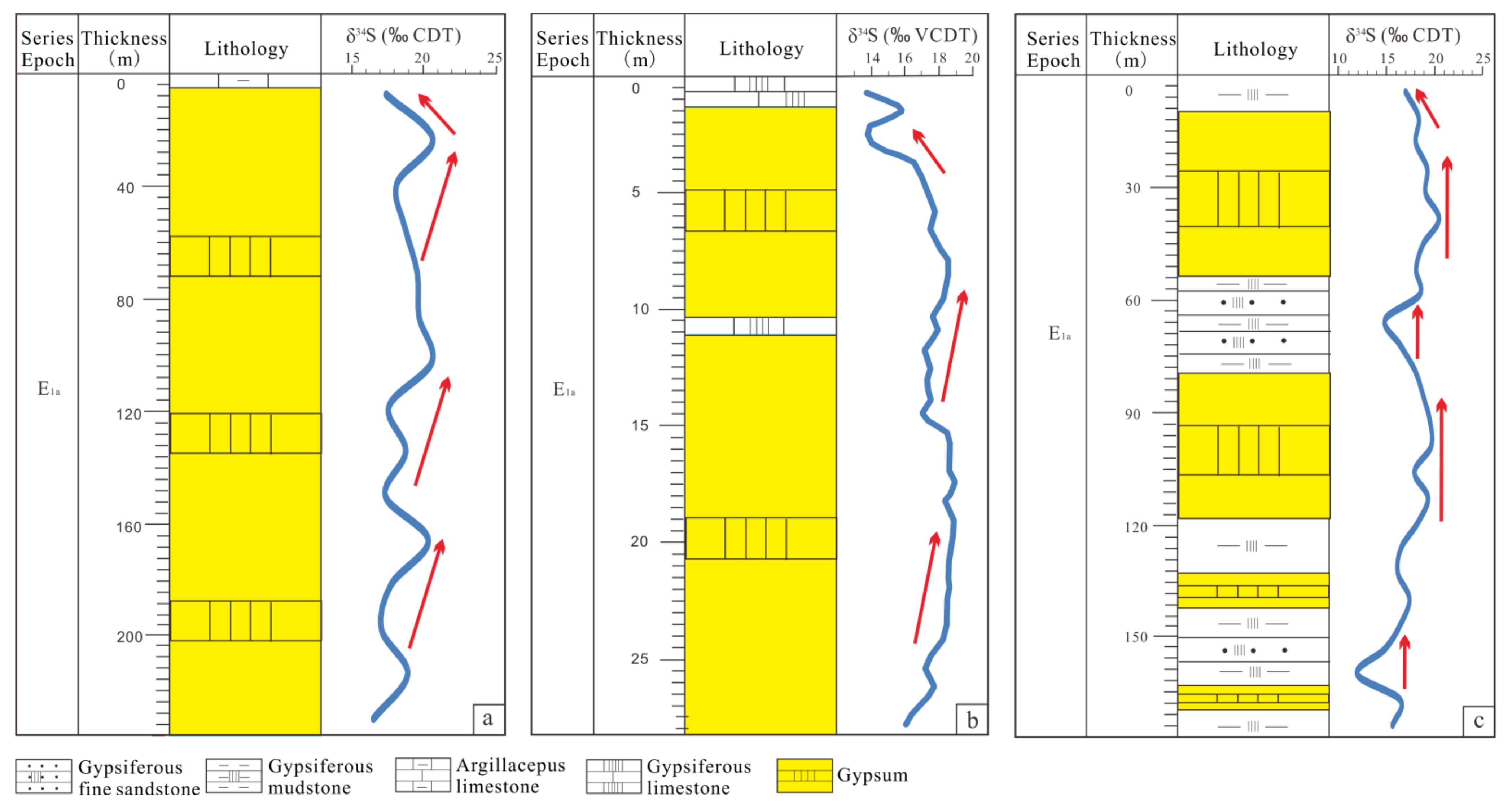
5.2. Sulfur Isotopic Fluctuation of Gypsum in the Yarkand Basin in the Paleocene

Three sulfur isotopic curves with gradually increasing (or decreasing) trends can be observed clearly in Figure 4. Combined with the values of sulfur isotope (Table 1 and Table 2), from the bottom to the top of the AET profile, the curve showed three fluctuation trends: 16.6‰−20.3‰, and 17.4‰−20.5‰, then slowly reduced to 18.2‰, and increased to 20.6‰, ultimately decreasing to 17.5‰. Three cycles showing a down-up trend and a primarily marine depositional environment are revealed in the AET profile. Similarly, the δ34 S values of samples in the DSK profile fluctuated from 15.9‰ to 19.8 ‰, then declined to 15.0‰, then steadily increased to 20.6‰, and then gradually decreased to 17.1‰, which may reflect the two cycles from interactive marine–terrestrial to the marine sedimentary environment during the period. Compared with the above two profiles, the sulfur isotopic curve is also presented with two waved trends in the KLY profile. The variation range of values are 16.2‰−19.0‰ and 17.7‰−18.3‰ respectively, declining to 16.5‰, and lastly persistently declined to 13.8‰.
The gradually increasing trend of sulfur isotopic composition was previously interpreted as the expansion of transgressive extent in the evaporites basin [37,46,47,48], but it is perhaps not true. The evaporites such as gypsum and halite usually occur in a closed or semi-closed basin, and in an arid climate or intensely evaporative surroundings. The fluctuation in δ34 S values is usually caused by bacterial sulfate reduction or a lack of sufficient/continual supplement of seawater in the closed evaporites basin, but normally no more than ±2‰ [7,49,50,51], and the sulfur isotopic composition is kept steady range with the persistent supplement of seawater in nearly semi-closed basin as lagoon. If a sudden expansion of transgressive extent in evaporites basin had occurred, the salinity of water in ancient saline lakes would be reduced; accordingly, a depositional termination of evaporites appeared. There is a nearly successive deposition of gypsum in the profiles of KLY (Figure 2a,b,e and Figure 4a) and AET (Figure 2c,f and Figure 4b) except DSK profile (Figure 2d and Figure 4c), which indicates that the seawater cannot have entered into the Yarkand ancient saline lake in this stage. The increasing values of sulfur isotopic composition reflect that enrichment of δ34 S occurred in seawater sulfate, and indicate oxidation or bacterial reduction of seawater sulfide in the Paleocene. On the one hand, these may be a hint of slowly increasing oxygen content in the air; meanwhile, the terrestrial sulfide decreased in the ancient ocean. Considering the three profiles, at least three events involving oxidation of seawater sulfide occurred, and perhaps three oxygen-enriched events might have existed in the Paleocene. However, on the other hand, it has now been established that considerable sulfur-isotope fractionation occurs in the biological sulfur cycle and that the bacterial reduction of sulfate, which leads to the enrichment of S34 in sulfate and its depletion in sulfide, and is largely responsible for the wide fluctuations in isotope ratios which occur in marine sediments [52]. Furthermore Boschetti et al. [50,51] have verified that an increase of δ34 S in gypsum results in bacterial sulfate reduction (δ34 S increased in residual dissolved sulfate and then deposition occurred again).
The δ34 S values of samples in the DSK profile range from 12.2‰ to 20.6‰, which belongs to the marine and interactive marine-terrestrial sedimentary environment [43,44], and may reflect the two times of transformation from interactive marine-terrestrial to the marine sedimentary environment during the period. Compared with the AET and KLY areas, the DSK area might be high-relief topography, and is nearer the South Tianshan piedmont, and it is possible that abundant terrestrial freshwater enriched sulfide from the piedmont had been injected into the ancient saline basin during that period. In the same way, the KLY area might be higher ancient topography than that of the AET area for its two waved trends and the gypsiferous mudstone interbedded in the profile is also verified (Figure 4).
On the top of three profiles (AET, DSK, and KLY), the same trend in which the values of the sulfur isotope gradually decreased occurred at the end of the Paleocene, the values decreased to 17.5‰ (δ34 SCDT), 17.1‰ (δ34 SCDT) and 13.8‰ (δ34 SVCDT) respectively. The sulfur isotopic composition in AET and DSK regress to the initial datum of the bottom profiles (17.5‰ and 17.1‰), but 13.8‰ in KLY, which might hint that sulfate reduction in near-shore organic material occurred or terrestrial fragments of sulfide were carried to the saline lake by freshwater rooted in peripheral rivers of the basin in the end.
Due to the difficulty involved in the collection of gypsum rock debris (or core) from coorporation-owned oil fields, only five samples of borehole debris are collected to analyze sulfur isotopic composition. The range of sulfur isotopic values in the five boreholes is quite narrow compared with the three profiles. It is from 16.6‰ to 19.1‰ (δ34 SCDT), and the mean is 17.5‰, approaching the total mean of 17.7‰ (97 samples in the basin). The cause might be a short interval or a small number of samples collected. Though the samples were located in different parts of the borehole profiles, the sulfur isotopic values are fluctuant around the mean of 17.5‰. It is clear that the values of the sulfur isotope in the Wb1 and Wx1 boreholes are higher than these of Minc1, Mac1, and Tc2 boreholes, which hints that the ancient seawater must come from the northwestern Yarkand Basin, and all the other borehole areas were far away from the seawater estuary in the basin in the Paleocene.

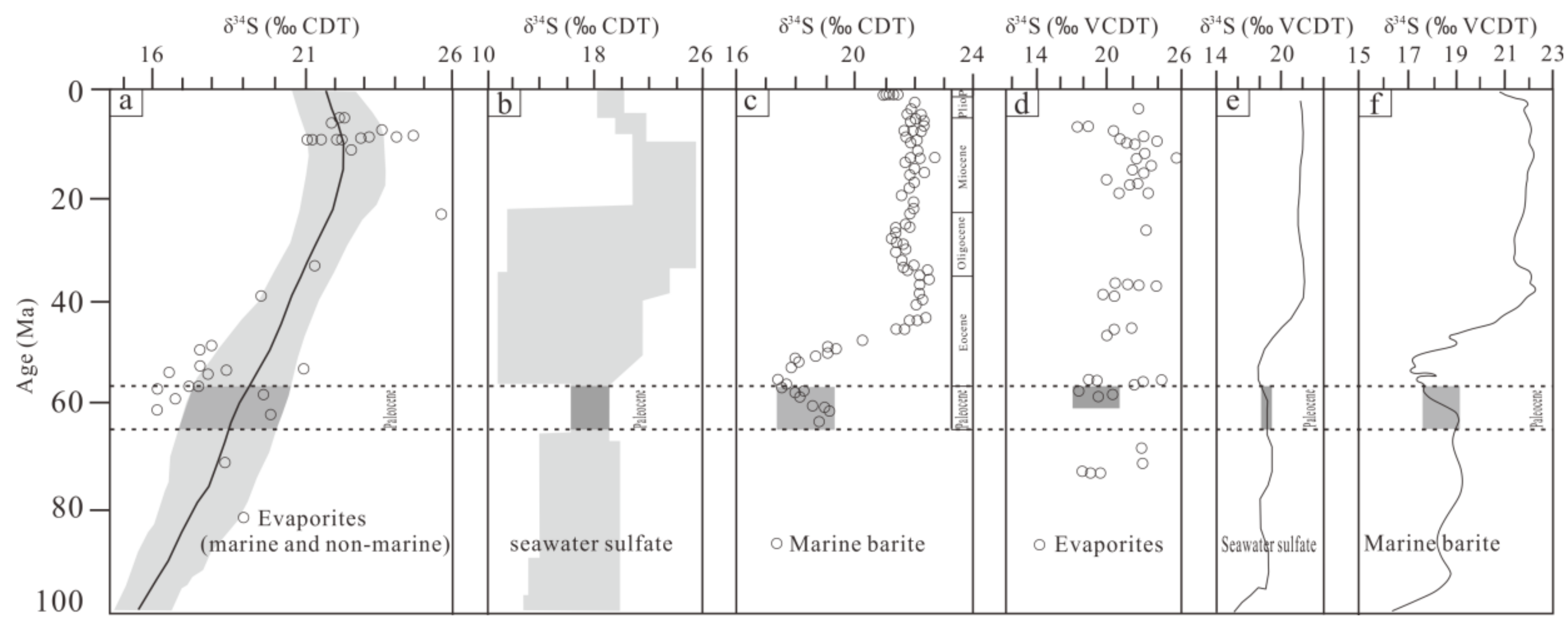
5.3. Depositional Environment and Sulfur Isotopic Composition on the Eastern Paratethys Seawater in the Paleocene

The Paleocene Aertashen Formation is stable in thickness and widespread in the Yarkand basin [40]. In the Paleocene, seawater had been invaded from the Alay graben in the northwest of Tarim Basin, then blocked by the middle-low hills of West Kunlun Mountain, forming a lagoon in Yarkand Basin. The semi-closed lagoon with a water depth of 20–50 m, and a hot-arid climate [53,54], lagoon facies, and very shallow-water evaporation-platform facies were developed [34]. In the Paleocene, the Yarkand basin was a depression [24], which was controlled by the tectonic framework initiated during the Late Cretaceous and the flexure deformation of the piedmont thrust belt in the foreland basin. The subsided and depositional center of this basin was located at the West Kunlun piedmont, and the deposits gradually thinned along the SW-NE orientation in the basin [25]. Though the topography of the ancient saline lake was higher in the eastern part than that in the western, the evaporites at the edge of this saline basin were similar in thickness except for the area of bore Wx1 and Wb1 (the thickness of gypsum may be influenced by tectonic compression). For instance, the thickness of the evaporites is between 58–96 m (78.0 m averaged) at the South Tianshan piedmont, between 6–231 m (average 64.5 m average) at the West Kunlun piedmont, and that at the Markit slope is between 17–131 m (60.1 m average) (Table 3). The isopach map of gypsum is seen in Figure 1a. There are five main depositional centers of gypsum in the basin, two in the South Tianshan piedmont (the areas of Wx1 and DSK), two in the West Kunlun piedmont (the areas of Wb1 and AET), and one in the Markit slope (the areas of Q6 and Tc2) (Figure 1a).
It is difficult to confirm the sulfur isotopic composition of evaporites of the ancient ocean in the same geological epoch because of the dispersive component of the world. However, to date, research results verifies that sulfur isotopes of seawater sulfate can be a useful tool for stratigraphic correlations. Secular data of seawater sulfur isotopes archived in evaporite, carbonate-associated sulfate, and marine barite from worldwide locations allow reconstruction of a continuous seawater sulfate sulfur isotopic curve for the Phanerozoic [55]. The Yarkand Basin, as a northeastern part of the eastern Paratethys ocean, in which evaporites nearly successive deposited and directly recorded the evolutionary history of the sulfur isotope in eastern Paratethys seawater. Thode [52] had identified the minimum sulfur isotopic values as the δ34 S of global seawater about the evaporites stratum with the same geological epoch and in different areas because of the consistency of the minimum values, and the other values were interpreted by regional characteristics of sulfate reduction action. However, it is in conformity with results from the Caspian Sea and Rhine Graben evaporites basins, and some means are higher than the actual value of ancient seawater [7]. Combined with the latest published data and LOWESS curve of sulfur isotope (from 66.06 ± 0.3 Ma to 56.13 ± 0.2 Ma) [45], we tried to obtain the evolution of Eastern Paratethys seawater using the sulfur isotopic composition of gypsum in the Paleocene. In this paper, we think that some abnormal values need to be rejected when the sulfur isotopic composition of ancient seawater is estimated as the values (near or less than 10‰) of evaporites samples occurring in terrestrial facies surroundings, and other isotopic (Sr, C, and O, etc.) analysis is needed under beneficial conditions, such as improved funding for research.
The sulfur isotopic values (δ34 SCDT or δ34 SVCDT) of global marine sulfate ranges about from 16.2‰−21‰ in the Paleocene (Figure 3), and the mean of the mid-values is 18.4‰. However, in the Yarkand Basin in the Paleocene, the range of values is from 12.2‰ to 20.6‰ (δ34 SCDT or δ34 SVCDT), and the mean is 17.7‰. It is relatively lower compared with global data, and can be observed clearly in Figure 5 (sulfur isotopic curves of marine gypsum and barite from the last c.66 Ma–56 Ma). Though some fluctuations occurred in the four curves, the general trend of a single curve can be identified easily in the figure. The sulfur isotopic curves show the same trend of overall decrease between of KLY profile and global LOWESS curve for about the last 66 Ma–56 Ma generated from barite data, similarly to the curves of the AET and DSK profiles with an overall increasing trend. Comparing with the four sulfur isotopic curves, the reason for the differences in the overall trend is not clear, especially with KLY, AET, and DSK profiles in the same basin. The two areas of AET and DSK were perhaps located in different depositional environments and influenced by the biological sulfur cycle (the bacterial reduction of sulfate).
Considering the data of only the marine depositional environment in the basin (the values equal to or greater than 15‰ selected [43,44,45]), if some values are discounted, such as KLY-G35, G36, and G38, and DSK-G3, then the new range is 15.0‰ to 20.6‰ in the Yarkand Basin, the mean of total 93 samples is 17.9‰, and the sulfur isotopic values of Yarkand Basin clearly approach the data of global marine sulfate (18.4‰). Considering only the latest data [45], the mean is 18.3‰ from about the last 66–56 Ma, and the same values are also approached. Considering the overall downward trend of sulfur isotopic composition during the Paleocene (Figure 5) and three up-down fluctuations at least in the basin, we possibly infer that sulfur isotopic composition (δ34 SCDT or δ34 SVCDT) in the seawater of the northeastern part of the eastern Paratethys ocean was about 15.0‰ to 20.6‰, and 17.9‰ averaged in the Paleocene. Synthetically, considering the global sulfur isotopic composition of seawater, the final range might be from 15.0‰ to 21.0‰, with 17.9‰−18.3‰ averaged in the Paleocene. Therefore, the data of sulfur isotopic composition in the paper are a supplement for the global ancient seawater in the Paleocene. Moreover, sulfur isotopes can also better reflect the changes in the marine-terrestrial depositional environment. By the study of sulfur isotope geochemistry of gypsum in the profile of the evaporites basin, the paleo-sedimentary environment and its changes can be revealed.

6. Conclusions

The Yarkand Basin with the trumpet-shaped bay belongs to the northeastern part of eastern Paratethys ocean, in which a suite of evaporitic sequences was continuously developed and composed of massive gypsum interbedded fragmental rocks in the Paleocene. The values of sulfur isotopic composition are from 12.2‰ to 20.6‰ (δ34 SCDT or δ34 SVCDT), the mean is 17.7‰ in total of 97 gypsum samples. Considering the three profiles, the three-fold increase in the values of sulfur isotopic composition demonstrate that enrichment of δ34 S occurred in seawater sulfate, and hint that at least three episodes of oxidation or bacterial reduction of seawater sulfide occurred in the Paleocene, and three oxygen-enriched events or the biological sulfur cycle might exist in this epoch. The sulfur isotopic composition (δ34 SCDT or δ34 SVCDT) in the seawater of the northeastern part of the eastern Paratethys ocean was about 15.0‰ to 20.6‰, and 17.9‰ averaged in the Paleocene. Therefore, the ultimate range of global sulfur isotopic composition of seawater might be from 15.0‰ to 21.0‰, with 17.9‰–18.3‰ averaged in the Paleocene. which is a supplement for the global ancient seawater in the Paleocene.

Author Contributions

J.W. performed the data analyses and wrote the manuscript; Y.C. helped perform the analysis with constructive discussions. All authors have read and agreed to the published version of the manuscript.

Funding

The study was supported by the National Natural Science Foundation of China (No. 41972082), Major Projects of Xinjiang Uyghur Autonomous Region of China (No. 2020A03005–2), Compilation on Regional Geological Annals of China and Series Maps (No. DD20221645), and Compilation and Renewal on Series Maps of International Geoscience (No. DD20221648).

Data Availability Statement

The experimental datum used to support the findings of this study are included in the manuscript.

Acknowledgments

We appreciate two anonymous reviewers for their constructive comments and suggestions. Yaping Li and Tingdong Li gave many constructive suggestions and revised the paper. Wenjun Cheng is also thanked for assistance in sample collection.

Conflicts of Interest

The authors declare no conflict of interest.

References

  1. Holser, W.T.; Schidlowski, M.; Mackenzie, F.T.; Maynard, J.B. Geochemical cycles of carbon and sulfur. In Chemical Cycles in the Evolution of the Earth; Gregor, C.B., Garrels, R.M., Mackenzie, F.T., Maynard, J.B., Eds.; Wiley Press: New York, NY, USA, 1988; pp. 105–173. [Google Scholar]
  2. Berner, R.A.; Canfield, D.E. A new model for atmospheric oxygen over Phanerozic time. Am. J. Sci. 1989, 189, 333–361. [Google Scholar] [CrossRef] [PubMed]
  3. Strauss, H. The isotopic composition of sedimentary sulfur through time. Palaeogeogr. Palaeocl. 1997, 132, 97–118. [Google Scholar] [CrossRef]
  4. Petsch, S.T.; Berner, R.A. Coupling the geochemical cycles of C, P, Fe, and S: The effect on atmospheric O2 and the isotopic records of carbon and sulfur. Am. J. Sci. 1998, 298, 246–262. [Google Scholar] [CrossRef]
  5. Paytan, A.; Kastner, M.; Campbell, D.; Thiemens, M.H. Sulfur isotopic composition of Cenozoic seawater sulfate. Science 1998, 282, 1459–1462. [Google Scholar] [CrossRef] [PubMed]
  6. Paytan, A.; Kastner, M.; Campbell, D.; Thiemens, M.H. Sea water sulfur isotope fluctuations in the Cretaceous. Science 2004, 304, 1663–1665. [Google Scholar] [CrossRef] [PubMed]
  7. Holser, W.T.; Kaplan, I.R. Isotope geochemistry of sedimentary sulfates. Chem. Geol. 1966, 1, 93–135. [Google Scholar] [CrossRef]
  8. Holser, W.T. Catastrophic chemical events in history of ocean. Nature 1977, 267, 403–408. [Google Scholar] [CrossRef]
  9. Claypool, G.E.; Holser, W.T.; Kaplan, I.R.; Sakai, H.; Zak, I. The age curves of sulfur and oxygen isotopes in marine sulfate and their mutual interpretation. Chem. Geol. 1980, 28, 199–260. [Google Scholar] [CrossRef]
  10. Hurtgen, M.T.; Arthur, M.A.; Suits, N.S.; Kaufman, A.J. The sulfur isotopic composition of Neoproterozoic seawater sulfate: Implications for a snowball Earth? Earth Planet. Sci. Lett. 2002, 203, 413–429. [Google Scholar] [CrossRef]
  11. Wu, N.P.; Farquhar, J.; Strauss, H. δ34 S and Δ33 S records of Paleozoic seawater sulfate based on the analysis of carbonate associated sulfate. Earth Planet. Sci. Lett. 2014, 399, 44–51. [Google Scholar] [CrossRef]
  12. Johnson, D.L.; Grossman, E.L.; Webb, S.M.; Adkins, J.F. Brachiopod δ34 SCAS microanalyses indicate a dynamic, climate-influenced Permo-Carboniferous sulfur cycle. Earth Planet. Sci. Lett. 2020, 546, 116428. [Google Scholar] [CrossRef]
  13. Yuan, J.Q.; Huo, C.Y.; Cai, K.Q. The high mountain-deep basin saline environment-a new genetic model of salt deposits. Geol. Rev. 1983, 29, 159–165. [Google Scholar]
  14. Yuan, J.Q. Proceedings of Salt Mine Geology of Jianqi Yuan Professor; Xueyuan Pub House: Beijing, China, 1989; pp. 1–227. [Google Scholar]
  15. Qian, Z.Q.; Qu, Y.H.; Liu, Q. Potassium Deposit; Geological Publishing House: Beijing, China, 1994; p. 11. [Google Scholar]
  16. Hay, R.L.; Kyser, T.K. Chemical sedimentology and paleoenvironmental history of Lake Olduvai, a Pliocene Lake in northern Tanzania. Geol. Soc. Am. Bull. 2001, 113, 1505–1521. [Google Scholar] [CrossRef]
  17. Warren, J.K. Evaporites through time: Tectonic, climatic and eustatic controls in marine and nonmarine deposits. Earth Sci. Rev. 2010, 98, 217–268. [Google Scholar] [CrossRef]
  18. Burtman, V.S. Cenozoic crustal shortening between the Pamir and Tien Shan and a reconstruction of the Pamir–Tien Shan transition zone for the retaceous and Palaeogene. Tectonophysics 2000, 319, 69–92. [Google Scholar] [CrossRef]
  19. Bosboom, R.E.; Dupont-Nivet, G.; Houben, A.J.P.; Brinkhuis, H.; Villa, G.; Mandic, O.; Stoica, M.; Achariasse, W.J.; Guo, Z.; Li, C. Late Eocene Sea retreat from the Tarim Basin (west China) and concomitant Asian paleoenvironmental change. Palaeogeogr. Palaeocl. 2011, 299, 385–398. [Google Scholar] [CrossRef]
  20. Bosboom, R.E.; Dupont-Nivet, G.; Grothe, A.; Brinkhuis, H.; Villa, G.; Mandic, O.; Stoica, M.; Huang, W.; Yang, W.; Guo, Z.; et al. Linking Tarim Basin sea retreat (west China) and Asian aridification in the late Eocene. Basin Res. 2014, 26, 621–640. [Google Scholar] [CrossRef]
  21. Cao, Y.T.; Liu, C.L.; Jiao, P.C.; Zhang, H.; Wu, K.; Sun, H.W.; Lu, F.L.; Su, Y. Evaporite deposition and potassium enrichment prospect from Upper Cretaceous to Paleogene in Yarkand Basin, Xinjiang. Miner. Depos. 2016, 35, 300–314. [Google Scholar]
  22. Zhang, Y. Uplift of Tibet Plateau and formation and evolution of the southwestern inTarim Basin. Xinjiang Petrol. Geol. 1999, 20, 6–10. [Google Scholar]
  23. Zhang, D.; Hu, J.; Meng, Y.; Zheng, M.; Fu, M. Characteristics of Qimugen thrust nappe structure in the southwestern Tarim Basin Xinjiang, China, and its relationship with hydrocarbon. Geol. Bull. China 2007, 26, 266–274. [Google Scholar]
  24. Fang, A.; Ma, J.; Wang, S.; Zhao, Y.; Hu, J. Sedimentary tectonic evolution of the southwestern of Tarim Basin and west Kunlun orogen since Late Paleozoic. Acta Petrol. Sina 2009, 25, 3396–3406. [Google Scholar]
  25. Wang, Y.; Fu, D. The sedimentary-tectonic evolution of the southwest Tarim Basin from Cretaceous to Paleogene. Acta Geol. Sina 1996, 17, 32–40. [Google Scholar]
  26. Qu, G.; Li, Y.; Li, Y. Structural segmentation and its factor in the southwestern Tarim Basin. Sci. China Ser. D 2005, 35, 193–202. [Google Scholar]
  27. Ding, D.; Luo, Y. Collision structures in Pamir region and reformation of Tarim Basin. Oil Gas Geol. 2005, 26, 57–63, 77. [Google Scholar]
  28. Sun, L. Sedimentary facies and exploration of petroleum of the early Cretaceous in Kuqa depression and southwest depression in Tarim Basin. J. Palaeogeogr. 2004, 6, 252–260. [Google Scholar]
  29. Jia, J. Sedimentary characteristics and palaeogeography of the early Cretaceous in Tarim Basin. J. Palaeogeogr. 2009, 11, 167–176. [Google Scholar]
  30. Zhuang, H.; Guo, F.; Zhou, X. Evolution of sedimentary environment in late Cretaceous, Kunlun Mountain front, Tarim Basin. J. Xi’an Univ. Sci. Technol. 2013, 33, 39–45. [Google Scholar]
  31. Ma, H.; Yang, Z. Evolution of the Cenozoic in southwestern Tarim Basin. Xinjiang Geol. 2003, 21, 92–95. [Google Scholar]
  32. Shao, L.; He, Z.; Gu, J.; Luo, W.; Jia, J.; Liu, Y.; Zhang, L. Lithofacies Palaeogeography of the Paleogene in Tarim Basin. J. Palaeogeogr. 2006, 8, 353–364. [Google Scholar]
  33. Zhou, Z.; Zhao, Z.; Hu, Z. Every Epoch in Tarim Basin; Science Press: Beijing, China, 2001; pp. 1–359. [Google Scholar]
  34. Wang, F.; Song, Z.; Wu, S. Atlas on Paleogeography and Zoology of Xinjiang Uygur Autonomous Region; China Cartographic Publishing House: Beijing, China, 2006; p. 186. [Google Scholar]
  35. Guo, X.; Wang, D.; Ding, X.; Ye, L. Discovery of Dinoflagellates from the Tuyiluoke formation in Tarim Basin. Geol. Rev. 2008, 54, 814–820. [Google Scholar]
  36. Shi, J.A.; Chen, G.J.; Wang, Q.; Xue, L.H. Sequence Stratigraphy, Sedimentary and Diagenetic Evolution in the Western Tarim Basin; Science Press: Beijing, China, 2001. [Google Scholar]
  37. Xi, D.P.; Cao, W.X.; Cheng, Y.; Jiang, T.; Jia, J.Z.; Li, Y.H.; Wan, X.Q. Late cretaceous biostratigraphy and sea-level change in the southwest Tarim Basin. Palaeogeogr. Palaeocl. 2016, 441, 516–527. [Google Scholar] [CrossRef]
  38. Zhao, Z.X.; Yong, T.S.; Jia, C.Z.; Zhang, Z.M. Stratum of Tarim Basin; Petroleum Industry Press: Beijing, China, 1997; pp. 1–207. [Google Scholar]
  39. Cao, Y.T.; Zeng, C.M.; Li, Q.; Zhu, L.c.; Fu, J.G.; Zhang, L.; Xiong, Z.L.; Zhang, H. Preliminary study on evolution of sedimentary environment in Early Paleocene in the Yarkand basin, Xinjiang. Acta Geol. Sina 2021, 96, 1369–1379. [Google Scholar]
  40. Cao, Y.T. Marine transgressive-regressive cycles and evolution on ancient saline lake in the northwestern Tarim Basin in the Paleocene, Xinjiang Province, China. Carbonates Evaporites 2022, 37, 21. [Google Scholar] [CrossRef]
  41. Thode, H.G.; Monster, J.; Dunford, H.B. Sulphur isotope geochemistry. Geochim. Cosmochim. 1965, 25, 159–174. [Google Scholar] [CrossRef]
  42. Гриненкo, В.А.; Гриненкo, Л.H. Sulfur Isotope Geochemistry; Zhao, R., Translator; Science Press: Beijing, China, 1980; pp. 1–242. [Google Scholar]
  43. Liu, C.; Cao, Y.; Yang, H.; Jiao, P.; Gu, Q. Discussion on Paleogene-Neogene environmental change of salt lakes in Kuqa foreland basin and its potash-forming effect. Acta Geol. Sina 2013, 34, 547–558. [Google Scholar]
  44. Zhang, H.; Liu, C.; Cao, Y.; Sun, H.; Wang, L. A Tentative Discussion on the Time and the Way of Marine Regression from Tarim Bay during the Cenozoic. Acta Geosci. Sina 2013, 34, 577–584. [Google Scholar]
  45. Paytan, A.; Yao, W.; Faul, K.L.; Gray, E.T. Sulfur isotope stratigraphy. In Geologic Time Scale; Elsevier B.V.: Amsterdam, The Netherlands, 2020; pp. 259–278. [Google Scholar]
  46. Liu, C.L.; Jiao, P.C.; Cao, Y.T.; Chen, Y.Z. Report on Large-Scale Minerogenetic Conditions and Prediction Technique of Potash in Tarim Basin; Institute of Mineral Resources, Chinese Academy of Geological Sciences: Beijing, China, 2010; pp. 1–471. [Google Scholar]
  47. Zeng, C.M.; Liu, C.L.; Zhang, L.; Cao, Y.T. Report on Sedimentary Evolution and Controlling Factors of Evaporite in Kashgar Sag and Its Surrounding Areas in Meso-Cenozoic; Institute of Mineral Resources, Chinese Academy of Geological Sciences: Beijing, China, 2015; pp. 1–163. [Google Scholar]
  48. Cao, Y.T.; Zeng, C.M.; Zhang, L.; Zhu, L.C. A rapid marine regression in the southwestern Tarim Basin in the latest Cretaceous: Comparison of two different evaporitic sequences in the Yarkand Basin, Xinjiang Province, China. Acta Geol. Sin.-Engl. 2021, 95, 1714–1724. [Google Scholar] [CrossRef]
  49. Van Driessche, A.E.; Canals, A.; Ossorio, M.; Reyes, R.C.; García-Ruiz, J.M. Unraveling the sulfate sources of (giant) gypsum crystals using gypsum isotope fractionation factors. J. Geol. 2016, 124, 235–245. [Google Scholar] [CrossRef]
  50. Boschetti, T.; Cortecchi, G.; Toscani, L.; Iacumin, P. Sulfur and oxygen isotope compositions of Upper Triassic sulfates from Northerm Apennines (Italy): Palaeogeographic and hidrogeochemical implications. Geol. Acta 2011, 9, 129–147. [Google Scholar]
  51. Boschetti, T.; Toscani, L.; Shouakar-Stash, O.; Iacumin, P.; Venturelli, G.; Mucchino, C.; Frape, S.K. Salt waters of the Northern Apennine Foredeep Basin (Italy): Origin and evolution. Aquat. Geochem. 2011, 17, 71–108. [Google Scholar] [CrossRef]
  52. Thode, H.G.; Monster, J. Sulfur-isotope geochemistry of petroleum, evaporites, and ancient seas. In Fluids in Subsurface Environments; Young, A., Galley, J.E., Eds.; AAPG Memoir: Tulsa, OK, USA, 1965; Volume 4, pp. 367–377. [Google Scholar]
  53. Yong, T.S. Lithofacies and paleogeography of the late Cretaceous-Paleogene of the Tarim platform. Exp. Explor. Petrol. Geol. 1984, 6, 9–17. [Google Scholar]
  54. Yong, T.S.; Shan, J.B. The development and formation in the Tarim Basin in Cretaceous-Paleogene ages. Acta Sedimentol. Sin. 1896, 4, 67–75. [Google Scholar]
  55. Yao, W.Q.; Wortmann, U.G.; Paytan, A. Sulfur isotopes-use for stratigraphy during times of rapid perturbations. Stratigr. Timescales 2019, 4, 1–33. [Google Scholar]
Figure 1. (a) Isopach map of gypsum, gypsum outcrops, boreholes of gypsum occurred in the Yarkand basin in the Paleocene; (b) Tectonic sketch map of the Yarkand Basin.
Minerals 12 01031 g001
Figure 2. Three main marine sulfate outcrops and mineral characteristics of gypsum in KLY outcrop in the Yarkand Basin (Gyp: Gypsum. Hl: Halite). (a) Keliyang (marked by KLY) gypsum outcrop with underlying Tuyiluoke formation (Late Cretaceous) and overlying Qimugen formation (early Eocene); (b) photograph of part of the panel a; (c) Aertashen (marked by AET) gypsum outcrop; (d) Dashankou (marked by DSK) gypsum outcrop; (e) gypsum of KLY outcrop; (f) gypsum of AET outcrop; (g) gypsum of KLY sample; (h) SEM image of KLY sample with grey white halite in the gypsum; (i) EDS spectrum graphs.
Minerals 12 01031 g002
Figure 3. Sulfur isotopic variations of seawater sulfate in the Paleocene. (a) The values of δ34 SCDT range about from 17.2‰–20.4‰ [9]; (b) The values of δ34 SCDT range about from 16.2‰–19.1‰ [3]; (c) The values of δ34 SCDT range about from 17.4‰–19.3‰ [5]; (d) The values of δ34 SVCDT range from about 17.0‰–21.0‰ [12]; (e) The values of δ34 SVCDT range about from 18.1‰–19.1‰ [11]; (f) The values of δ34 SVCDT range about from 17.34‰ ± 0.2–19.11 ± 0.3‰ [45].
Minerals 12 01031 g003
Figure 4. The sulfur isotopic curve of marine gypsum in the Yarkand Basin in the Paleocene. (a) AET profile; (b) KLY profile; (c) DSK profile.
Minerals 12 01031 g004
Figure 5. Sulfur isotopic curves of marine gypsum and barite. The cinereous LOWESS curve from the global marine barite data from the last c.66 Ma–Ma [45]. The blue, red, and green curves are from the data of AET, DSK, and KLY gypsum profiles of the Yarkand Basin during the Paleocene, respectively.
Minerals 12 01031 g005
Table 1. Sulfur isotopic composition of seawater gypsum in the Paleocene [39,40].
Samplesδ34 S
(‰, CDT)
Samplesδ34 S
(‰, CDT)
Samplesδ34 S
(‰, CDT)
Samplesδ34 S
(‰, CDT)
AET-G1517.5DSK-G2617.1DSK-G1118.1Wb1–619117.8
AET-G1420.6DSK-G2518.4DSK-G1019.5Wb1–619518.2
AET-G1318.2DSK-G2418.0DSK-G918.4Wb1–619619.1
AET-G1218.7DSK-G2319.3DSK-G816.7Minc1–368517.0
AET-G1119.6DSK-G2219.2DSK-G716.4Minc1–368617.2
AET-G1019.7DSK-G2120.6DSK-G617.6Minc1–368717.2
AET-G920.5DSK-G2018.9DSK-G516.7Minc1–368817.1
AET-G817.6DSK-G1918.2DSK-G415.1Minc1–368917.2
AET-G718.8DSK-G1818.6DSK-G312.2Mac1–205116.6
AET-G617.4DSK-G1715.0DSK-G216.7Mac1–205216.6
AET-G520.3DSK-G1616.6DSK-G115.9Mac1–205316.9
AET-G417.8DSK-G1518.1Wx1–356017.6Tc2–444117.7
AET-G317.1DSK-G1419.0Wx1–358317.9Tc2–447416.8
AET-G218.9DSK-G1319.7Wx1–358817.7Tc2–447817.7
AET-G116.6DSK-G1219.8Wx1–364018.1
Table 2. Sulfur isotopic composition of gypsum in KLY outcrop in the Paleocene.
Samplesδ34 S
(‰, VCDT)
Samplesδ34 S
(‰, VCDT)
Samplesδ34 S
(‰, VCDT)
KLY-G3813.8KLY-G2517.7KLY-G1218.8
KLY-G3715.8KLY-G2417.9KLY-G1118.7
KLY-G3613.9KLY-G2317.2KLY-G1018.6
KLY-G3514.0KLY-G2217.5KLY-G918.7
KLY-G3416.5KLY-G2117.3KLY-G818.5
KLY-G3317.0KLY-G2017.5KLY-G718.5
KLY-G3217.4KLY-G1917.1KLY-G618.3
KLY-G3117.8KLY-G1818.5KLY-G517.6
KLY-G3017.5KLY-G1718.6KLY-G417.2
KLY-G2918.0KLY-G1618.6KLY-G317.8
KLY-G2818.6KLY-G1519.0KLY-G216.8
KLY-G2718.4KLY-G1418.4KLY-G116.2
KLY-G2618.3KLY-G1318.9
Table 3. Thickness of gypsum in the Yarkand Basin in the Paleocene.
BoreholesThickness (m)BoreholesThickness (m)BoreholesThickness (m)
Wx1164P16Md117
Wb1253Ps228H237
Ak158Ks101108H352
Ak280Kd154Sh248
Ys1101Kd10174Ln126
S110Minc129Tc2131
T140Mac162Q6110
DSK96AET231KLY28.4
Notes: All the data are from Cao (2022) expect for DSK (96 m), AET (231 m) and KLY (28.4 m) profiles.
Publisher’s Note: MDPI stays neutral with regard to jurisdictional claims in published maps and institutional affiliations.

