Knothe Time Function Optimization Model and Its Parameter Calculation Method and Precision Analysis

Abstract

Considering the shortcomings of the currently used time functions for dynamically predicting surface mining subsidence and calculating its parameters, a novel time function is proposed on the basis of an in-depth analysis on the movement characteristics of mining surface points in a fully mined area and the measured mining subsidence data in the field during the course of the mining process. The proposed function can be used to effectively characterize the surface subsidence, the subsidence velocity, and the acceleration of the mining area. All the parameters involved in the function have their physical meaning, and their influence on the function was also analyzed in this study. A parameter calculation method is proposed for the new time function based on the normalization method and least square principle. Taking the measured dynamic subsidence data of 22,618 working faces in a coal mine as an example, the reliability of the new time function model was verified by comparing the measured data with the predicted results. The results show that the average relative root-mean-square error was 5.2%, and the prediction accuracy was improved compared with the Knothe time function, double-parameter Knothe time function, and piecewise optimized Knothe time function.

1. Introduction

Surface mining subsidence is a complicated process that changes in time and space [1,2,3,4]. With the advancement of the working face, the relative positions of the working face and surface points vary with time, and the influence of mining on the surface points also changes [5,6,7]. The movement of a fixed mining surface point experiences a process including the starting movement, violent movement, and stop movement [8,9,10]. In practice, a situation that we often encounter is that the practical problems cannot be adequately solved on the basis of the final state of the surface subsidence law. Therefore, it is necessary to conduct further studies on the dynamic surface subsidence law [11,12]. For example, in supercritical mining conditions, a flat bottom shows up in a subsidence basin, and all points in this flat bottom have almost the same magnitude of subsidence, but only a small surface deformation can be observed. However, buildings in this area cannot be considered undeformed or undamaged. Each point in the area experiences a dynamic deformation process. Even though such dynamic deformation is momentary, it has the potential to ruin the building. When conducting mining activities under buildings, it is necessary to determine the start time at which the buildings are affected, as well as the amount of surface movement and deformation at different times, in order to take appropriate measures to protect the buildings, such as enhanced observation, reinforcement, temporary relocation, or change of use. Therefore, the dynamic prediction of surface mining subsidence is of great practical significance to mining engineering [13,14,15].

Most existing models for dynamic prediction are based on a combination of the static prediction model and the corresponding time function. The static prediction model for surface mining subsidence has been well developed; thus, determining the time function in accordance with the actual surface mining subsidence is the key to improve the precision of dynamic prediction of the surface mining subsidence [16,17]. Accordingly, many scholars carried out relevant studies. Knothe established the Knothe time function model on the basis of Mitscherlich’s growth law, which has only one parameter and can be easily used to predict the dynamic surface subsidence, but it has shortcomings in reflecting the change law of surface subsidence velocity and acceleration [18,19,20,21,22,23]. Given the deficiency of the Knothe time function, Sroka developed a new time function, which can reflect the law of surface subsidence and its velocity [24], but it is difficult to obtain the parameters. From the viewpoint that there is a lag between surface behavior and underground mining, Kowalski proposed a generalized time function [25], which has three parameters, making up for the deficiency of the Knothe time function. However, this time function cannot effectively express the variation law of the surface subsidence velocity and acceleration, and some parameters have no clear physical meaning, leading to difficulties in calculating or measuring these parameters. Chang and Wang made an assumption that, when the subsidence velocity of a surface point reaches its maximum value, the subsidence of this point is roughly equal to half of its maximum subsidence. They constructed a piecewise Knothe time function which to some extent improved the accuracy of dynamic prediction of surface movement and deformation, as well as extended the application of the Knothe time function [26]. However, there are shortcomings in the model; the value of time function at the point of segmentation is not consistent with the theoretical value, and the maximum value of time function cannot converge to 1. Liu improved the Knothe time function by directly treating it with n power [27,28,29,30]. The improved model dramatically enhanced the description of surface mining subsidence characteristics, but it still had some deficits. The measured data showed that, when the surface subsidence rate reached the maximum, the surface subsidence usually reached about half of the maximum subsidence value, but the improved model could not express this characteristic, and the physical meaning of the model parameters was not studied in depth. Zhang and Cui optimized the piecewise Knothe time function [13], making up for the shortcomings of the original model as described above, but it was hard to determine the time at which the maximum subsidence velocity was reached, limiting the application of the piecewise Knothe time function. Therefore, the objective of this study was to improve the Knothe time function by overcoming its shortcomings so that it can be used to effectively characterize surface subsidence.

In the literature, studies on methods for calculating the parameters of time function for surface subsidence prediction have focused on the Knothe time function, including the graphical method, interval estimation method, and least square curve fitting method. Knothe first proposed the graphic method, which determines the parameters of the time function by selecting the subsidence observations of some surface points and plotting their subsidence–time curves [24,31]. The graphical method is feasible and straightforward, but its accuracy is limited by observation data and mapping. Thus, it is difficult to apply in practice. Cui constructed the interval estimation method for the Knothe time function parameter as a function of the general law of surface movement of mining subsidence [24], which can be used even when no measured data are available. Although the calculation result is an interval value and its accuracy cannot be guaranteed, the idea of using this method to calculate the parameters of the time function is worth affirming. The reason that the calculation result of this method is an interval value is that the critical full mining width adopted in this calculation model is an interval value. By finding a reliable and easy-to-calculate method for the critical full mining width, we can establish a high-precision method for determining the Knothe time function parameter according to the basic idea of the interval estimation method. In view of this, Hu used the angle of full subsidence to construct the critical full mining width and established a new Knothe time function model [1,32]. The above methods are feasible for the Knothe time function with only one parameter. However, other time functions have introduced additional parameters to make up for the deficiency of Knothe time function, posing a challenge for their obtention using the methods described above. To solve this issue, most researchers used curve fitting to find parameters on the basis of the measured data. However, we found that this method also has some drawbacks through repeated experiments, such as a large standard deviation of the parameters obtained by fitting, an unsatisfactory R-squared index value, and a wide range of fitting parameters, indicating that the current time function model and its method of calculating parameters still need to be further improved. In order to avoid these issues, in this paper, we rebuild the time function model for surface mining subsidence prediction and propose that the measured data should be normalized first. Curve fitting is then carried out to obtain a high-precision time function model and the results of the calculated parameters.

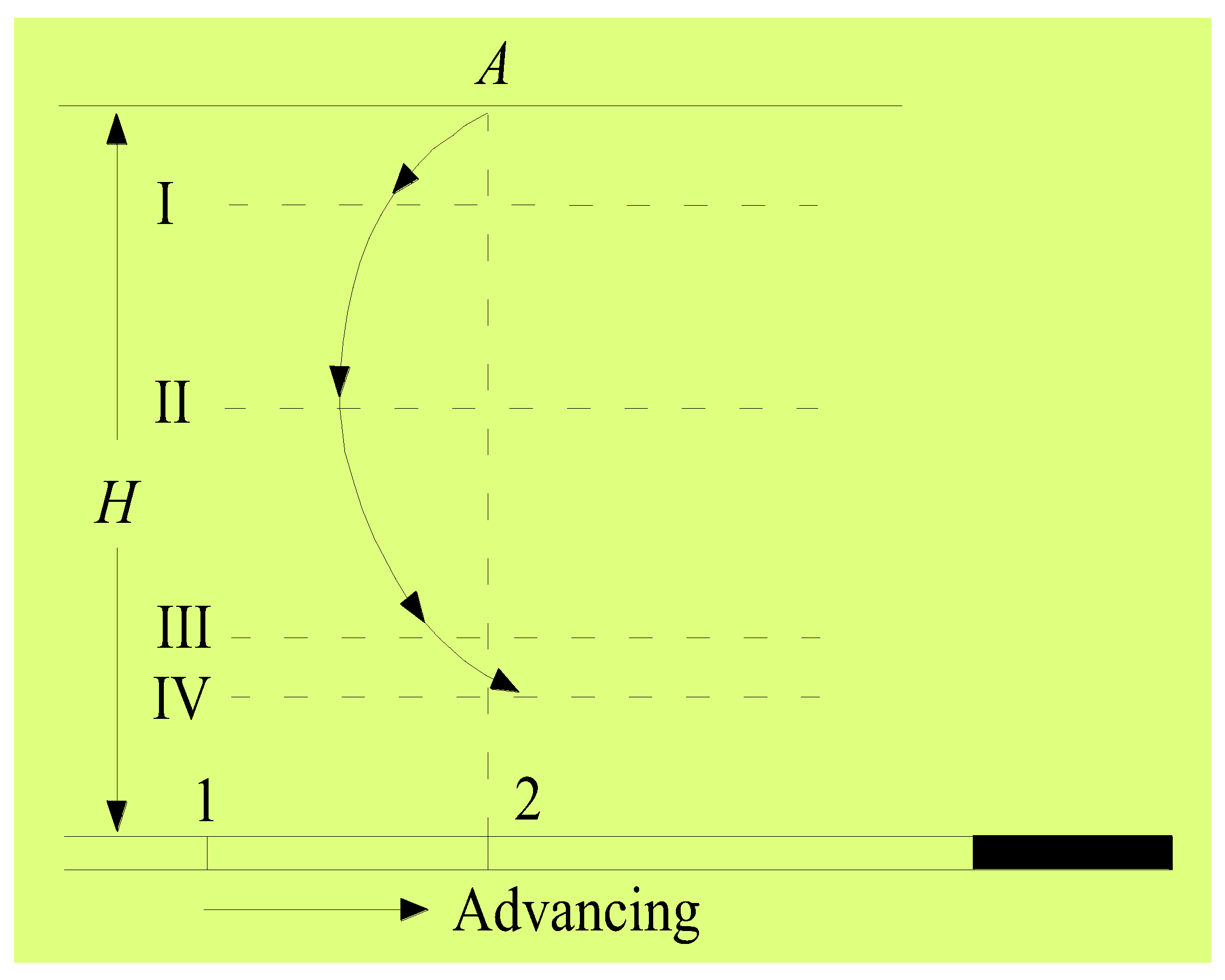
2. Analysis of Surface Point Movement Characteristics in Mining Process

In the study of mining subsidence, it is considered that the surface begins to subside when the surface observation point sinks 10 mm. Generally, during the first mining action, the mining effect reaches the surface and causes surface subsidence, while the distance from the open-off cut to the front of the working face is 1/4 H₀–1/2 H₀ (H₀ is the average mining depth). In the process of mining, the surface points go through a complicated process in time and space, i.e., from the beginning of the movement, through violent movement, to the gradual stopping of the movement, which can be divided into four stages, as described below. In this paper, the surface point A in the fully mined zone along the main strike section of a surface subsidence basin was taken as an example to illustrate the subsidence process in Figure 1 [12].

(1)

When the working face advances toward Point A, the surface subsidence spreads to point A, the surface subsidence speed increases, and the moving direction of point A is opposite to the advancing direction of the working face. This is the first stage of the movement.

(2)

When the working face continues to advance directly below Point A (e.g., location “2” in Figure 1), the surface subsidence rate increases rapidly and gradually reaches the maximum subsidence rate, and Point A moves nearly in the plumb direction. This is the second phase of the movement.

(3)

When the working face continues to advance and gradually moves away from Point A, the rate of surface subsidence decreases rapidly, and Point A moves in the same direction as the working face. This is the third stage of the movement.

(4)

When the working face is far from the surface point A, the influence of the working face on point A disappears gradually, and the movement of point A finally stops. This is the fourth stage of the movement.

In conclusion, the ideal time function should be able to describe not only the characteristics of the surface subsidence track, but also the velocity and acceleration of the surface subsidence.

3. Knothe Time Function and Two-Parameter Knothe Time Function

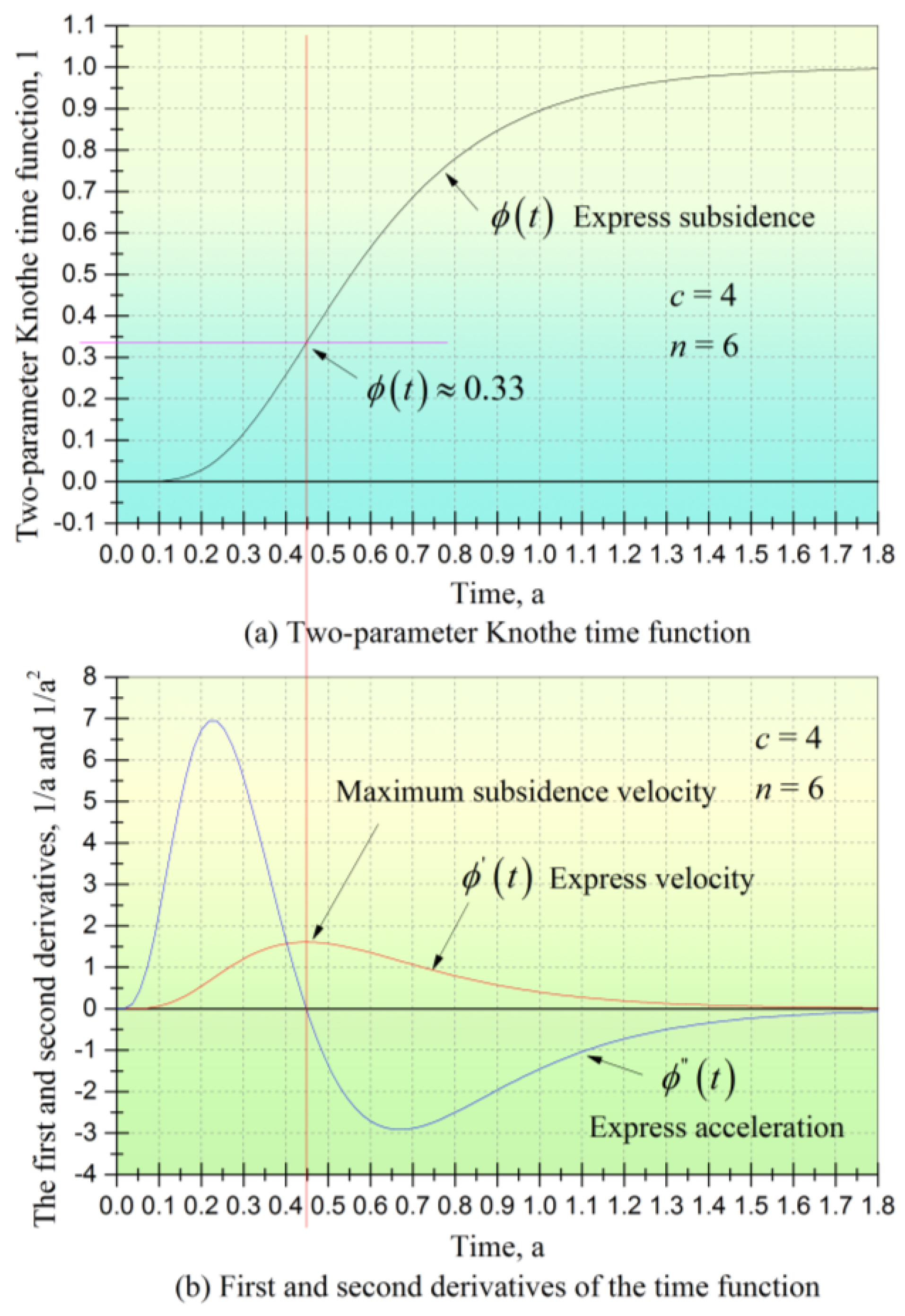
3.1. Knothe Time Function

Knothe established the Knothe time function model on the basis of Mitscherlich’s growth law [18,21]. The idea is to assume that the rate of subsidence $\frac{dW\left(t\right)}{dt}$ is proportional to the difference between the final subsidence $W_0$ and the dynamic subsidence $W\left(t\right)$ at a given time (see Equation (1)), and then to integrate Equation (1) according to the boundary condition of the initial time $t=0$ and $W\left(t\right)=0$ to get the subsidence expression of the dynamic process of surface movement, as expressed in Equation (2).

$$\frac{dW(t)}{dt}=c\times \left(W_0-W\left(t\right)\right),$$

(1)

where c is the influence coefficient of the time factors related to overburden lithology, with a dimension of 1/a.

According to the boundary conditions at the initial time $t=0$ and $W\left(t\right)=0$, integrating Equation (1) with t yields Equation (2).

$$W\left(t\right)=W_0\times \left(1-e^{-c\times t}\right).$$

(2)

$$W\left(t\right)=W_0\times \phi \left(t\right).$$

(3)

If $\varphi \left(t\right)=1-e^{-c\times t}$, then Equation (2) is transformed into Equation (3). In this model, $\varphi \left(t\right)$ is the Knothe time function of the surface subsidence, its first and second derivatives with respect to t are shown in Equations (4) and (5), respectively.

$${\phi }^{\prime }\left(t\right)=c\times e^{-c\times t},$$

(4)

$${\phi }^{″}\left(t\right)=-c^2\times e^{-c\times t},$$

(5)

where ${\phi }^{\prime }\left(t\right)$ is the first derivative of the Konthe time function, and ${\phi }^{″}\left(t\right)$ is the second derivative.

The Knothe time function and its first and second derivatives are plotted in Figure 2a,b, respectively.

It can be seen from Figure 2a that the Knothe time function can express the dynamic subsidence characteristics of the surface points to a certain extent, but the Knothe time function cannot reflect the characteristic that surface subsidence always lags behind underground mining. Figure 2b shows a graphical expression of the Knothe time function after calculating the first and second derivatives of time t. The physical meaning of the first derivative is the speed of the tangent slope change, while the physical meaning of the second derivative is the concavity and convexity of the function. In this study, they respectively represent the speed and acceleration of the surface mining subsidence. Combined with the above analysis, it can be seen that the variation characteristic of the surface subsidence speed should be $0\to +v_{\max }\to 0$, while the characteristic of subsidence acceleration should be $0\to +a_{\max }\to 0\to -a_{\max }\to 0$. Therefore, the first and second derivatives of the Knothe time function cannot effectively express the characteristics of subsidence velocity and acceleration of mining surface points.

3.2. Two-Parameter Knothe Time Function

Considering the deficiency of the Knothe time function, Liu added a power exponent n directly to the Knothe time function model, which is mathematically expressed in Equation (4) and defined as the “two-parameter Knothe time function” [27].

$$\varphi \left(t\right)={\left(1-e^{-c\times t}\right)}^n$$

(6)

where c is the lithologic parameter, and n is the parameter to be fitted.

The first and second derivatives with respect to t are shown in Equations (7) and (8), respectively.

$${\varphi }^{\prime }\left(t\right)=c\times e^{-c\times t}\times n\times {\left(1-e^{-c\times t}\right)}^{n-1},$$

(7)

$${\varphi }^{″}\left(t\right)=-n\times c^2\times e^{-c\times t}\times {\left(1-e^{-c\times t}\right)}^{n-1}+n\times \left(n-1\right)\times c^2\times e^{-2\times c\times t}\times {\left(1-e^{-c\times t}\right)}^{n-2}.$$

(8)

The two-parameter Knothe time function and its first and second derivatives are plotted in Figure 3a,b, respectively.

It can be seen from Figure 3a that the two-parameter Knothe time function can reflect the characteristics that the surface subsidence lags behind underground mining. As can be observed from Figure 3b, the two-parameter time function can also express the subsidence of the surface points and their movement velocity and acceleration to a certain extent. However, when the surface subsidence speed reaches the maximum, the surface subsidence value is only about 0.33 of the maximum value. Even if the parameters c and n take different values, the same results can still be obtained. However, the measured data show that, when the surface subsidence velocity reaches the maximum, the surface subsidence usually reaches about half of the maximum subsidence value, which is not in agreement with the result from the two-parameter Knothe time function. At the same time, Liu did not study the physical meaning of the parameters of the model, nor did he give an effective method to obtain the parameters of the time function. In addition, in the process of this study, when we use the model to carry out the least squares curve fitting practice based on the measured data, we find that there is not only a large value range of the fitted parameters in the same mining area, but also a significant error of the fitted indices (see Section 6.2). This can be attributed to the deficiency of the above two-parameter Knothe time function and the improper parameter calculation method. Therefore, although the research on the time function for dynamic prediction of surface mining subsidence has made important progress, further investigation is still needed to optimize the parameter estimation method.

4. Establishment of a New Time Function Model and Its Characteristic Analysis

4.1. Model Building

According to the above analysis, the time function for the dynamic prediction of surface mining subsidence should have the following characteristics: (1) the time function should be able to effectively express that the surface mining subsidence lags behind underground mining; (2) the value of the time function should increase and range from 0 to 1; (3) at the initial time t = 0, both the sinking velocity and its acceleration should be equal to 0; (4) in the intermediate stage of movement, the sinking velocity changes from $0\to +v_{\max }\to 0$, while the sinking acceleration varies from $0\to +a_{\max }\to 0\to -a_{\max }\to 0$; that is, as the time variable $t\to +\infty$, the sinking velocity and the acceleration both tend to 0.

Considering the deficiency of the above two-parameter Knothe time function and the subsidence, velocity, and acceleration characteristics of mining surface points, we analyzed the dynamic subsidence law of 32 observation points in Zhenchengdi Coal Mine, Malan Coal Mine, Guandi Coal Mine, and Tunlan Coal Mine in the Gujiao Mining Area, Taiyuan, China. It was found that the dynamic subsidence law of the surface points can be expressed using Equation (9), and a time function model for dynamic prediction of surface mining subsidence was then established. Equation (10) can be obtained by calculating the first derivative of Equation (9) with respect to t, which is the expression of subsidence velocity of the surface points. Equation (11) can be obtained by calculating the second derivative of Equation (9) with respect to t, which is the expression of subsidence acceleration of the surface points.

$$\mathsf{\Phi }\left(t\right)=1-e^{-c\times {(1.75\times t)}^n},$$

(9)

$${\mathsf{\Phi }}^{\prime }\left(t\right)=c\times n\times {1.75}^n\times t^{n-1}{e}^{-c\times {(1.75\times t)}^n},$$

(10)

$${\mathsf{\Phi }}^{″}\left(t\right)=c\times n\times (n-1)\times {1.75}^n\times t^{n-2}\times e^{-c\times {(1.75\times t)}^n}-c^2\times n^2\times {1.75}^{2n}\times t^{2(n-1)}\times e^{-c\times {(1.75\times t)}^n},$$

(11)

where c and n are the influence coefficients of time factors related to the mechanical properties of overburden, and their physical significance is shown in the next section.

4.2. Characteristic Analysis of New Time Function Model

Figure 4 shows that, when the surface subsidence velocity reaches the maximum, the new time function $\mathsf{\Phi }\left(t\right)\approx$ 0.49 conforms to the above surface mining subsidence law; that is, when the surface subsidence speed reaches the maximum, the surface subsidence usually reaches about half of the maximum subsidence value. Even if the values of parameters c and n are changed, the same results can still be obtained. At the same time, the new time function can effectively describe the above four characteristics of mining surface point subsidence. The results show that the new surface mining subsidence time function has certain advantages over the two-parameter Knothe time function. Figure 5 shows the adaptability analysis of the proposed time function. When c = 2 and n = 3, the time for the surface subsidence to lag behind underground mining is 0.05 a. When c = 4 and n = 3, the time lag between surface subsidence and underground mining is still 0.05 a; when c = 2 and n = 5, the time of surface subsidence lagging behind underground mining becomes 0.155 a. The above data show that, when the parameter n is constant, the time for the surface subsidence behavior to lag the underground mining is also constant, which shows that the parameter n plays a decisive role in the time when the surface subsidence behavior lags behind underground mining. At the same time, by comparing the change laws of function curves, when c = 2 and n = 3, and when c = 4 and n = 3, it can be seen that the parameter c plays a decisive role in the total time of surface subsidence. The above analysis shows that the new surface mining subsidence time function has strong universality.

5. Study on the Method of Model Parameter Estimation

Regarding the problem of obtaining the parameters of the time function for the dynamic prediction of surface mining subsidence, Cui suggested using the least squares method to fit the measured data. The time function parameters can be fitted by combining the time function with the static prediction model of surface mining subsidence to predict the relevant dynamic subsidence parameter values and comparing them with the measured values. However, since the static prediction model of surface mining subsidence also contains several parameters, the parameters of the time function obtained by fitting may be distorted.

Meanwhile, from the establishment process of the Knothe time function, we know that if the ratio (Equation (12)) of the dynamic subsidence to the final subsidence can be sorted out first, the curve fitting parameter of Knothe time function can be directly obtained. Therefore, in this study, we propose that the parameters of the new model (Equation (9)) can also be obtained using the following two steps: (1) normalize the measured data to get the ratio of the dynamic subsidence value to the final subsidence value of the surface point; (2) calculate the parameters by curve fitting. In this way, only the parameters of the time function are obtained, and the interference of other external parameters can be avoided. However, there is no curve fitting model for this function because the model is not a common function. In order to use the new model of this paper to calculate the parameters of curve fitting, we need to construct a multivariate function f (Equation (13)) using the new time function according to the least square principle, whose value will reach the minimum when the parameters determined are the best fitting parameters between the new model and the measured data. The remarkable advantage of this method is that it shows the fitting effect visually and analyzes the precision of parameters by checking the related fitting index (adjusted R-squared, standard error, etc.).

$$\mathsf{\Phi }\left(t\right)=1-e^{-c\times {(1.75\times t)}^n}=\frac{W\left(t\right)}{W_0},$$

(12)

$$f\left(c,n\right)={\displaystyle \sum _{i=1}^n{\omega }_i{\left[\mathsf{\Phi }\left(t\right)-\frac{W\left(t\right)}{W_0}\right]}^2=\min },$$

(13)

where ${\omega }_i$ is the weight function, and its default value is 1.

6. Research on Reliability and Effectiveness of Model

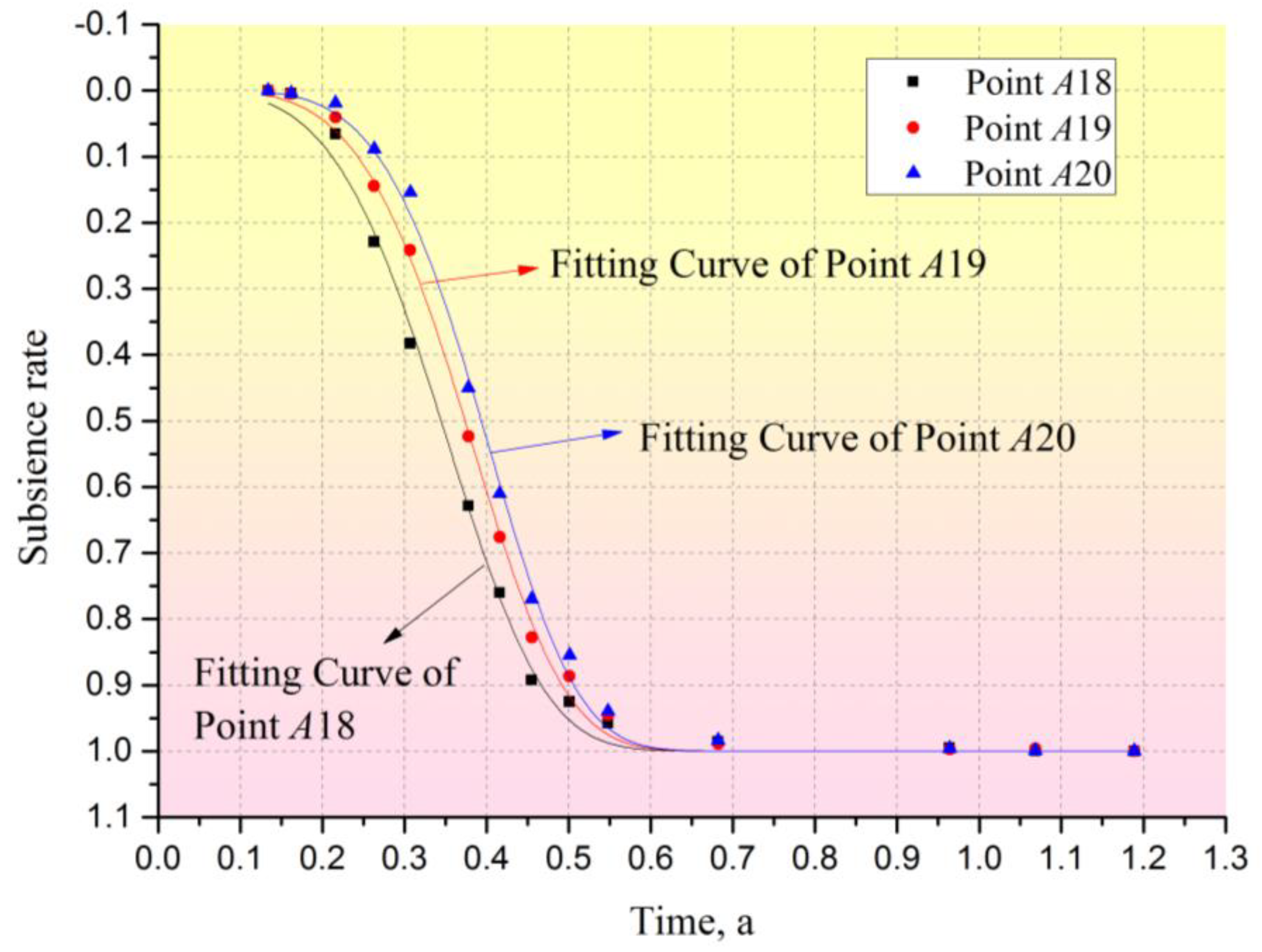
6.1. Introduction of Mining Area and Arrangement of Measured Data

In order to verify the reliability and effectiveness of the model and its parameter calculation method, we analyzed the measured data of surface mining subsidence of 22,618 working faces in a coal mine. The mine is located in the Gujiao mining area of Taiyuan, Shanxi Province. The topography of the mine is in the middle and low mountain areas. Most of the area is exposed bedrock except for the top part of the mountain covered with loess. The topography in the area is generally higher in the southwest and lower in the northeast with a relative height difference of 150–250 m. The peak and crest of the hill are relatively flat and covered with loess of the Cenozoic. The total of 22,618 working faces underwent mining on 1 March 2016. The coal seam is No. 3 coal in the well-field system, which has a thickness of 2.70–3.85 m and an average thickness of 3.40 m. The average dip angle of coal seam is 4°, the length of the longwall panel is 2092 m, and the dip width is 180 m. The ground elevation is 1135–1250 m, and the working face elevation is 721–800 m. The coal mining method is longwall mining.

In order to study the law of surface mining subsidence in the mining area, the most effective way is to lay observation lines directly on the surface above the working face, and the layout of observation lines should generally obey the following principles: (1) the observation lines should be laid on the main cross-section of the surface mobile basin; (2) the area where the stations are located should not be affected by the adjacent mining during the observation period; (3) the length of the observation lines should be larger than the extent of the surface mobile basin; (4) the observation points on the observation lines should have a certain density, which depends on the depth of mining and the purpose of the stations. Therefore, two observation lines and 42 monitoring points were set up by comprehensively considering the geological and geomorphological conditions above 22,618 working faces, the correlation of the surface and the subsurface, and the principle of convenience and validity of measurement. The distance between survey points was 30 m. One of the strike observation lines was located on the side of the open-off cut toward the main section, with a total of 26 monitoring points. The other dip observation line was located on the left of the fully mined area in the working face, with 16 monitoring points. Figure 6 shows the layout of the observation points. The other three datum points were located at the surface stability outside the mining subsidence-affected area.

During the period from 8 April 2016 to 8 May 2017, surface mining subsidence monitoring was carried out 14 times. The instrument used for monitoring was the Haixinda H32 GNSS receiver, and the monitoring method was the static measurement of GNSS. In order to reflect the dynamic characteristics of surface subsidence, this paper only takes the measured data from a part of monitoring points on the strike observation line as an example to carry out relevant research. Figure 7 shows the development of dynamic subsidence profiles in the longitudinal section of the face.

6.2. Reliability Analysis

As of 8 May 2017, the subsidence reached stabilization. For analyzing the reliability of the new time function model, the maximum subsidence point (A19) and its nearby monitoring points were selected as the research objects. The measured data of A16–A21 are shown in

Table 1. Measured dynamic subsidence data at point A16–A21.

Date	Monitoring Point
	A16	A17	A18	A19	A20	A21
8April 2016	0	0	0	0	0	0
28 April 2016	8	7	6	7	6	5
18 May 2016	199	144	87	55	26	17
4 June 2016	502	401	303	197	120	65
20 June 2016	787	644	506	330	209	110
18 July 2016	980	911	831	715	610	459
20 July 2016	1084	1054	1005	923	827	647
13 August 2016	1188	1197	1180	1130	1043	835
20 August 2016	1202	1225	1223	1210	1158	1007
16 September 2016	1216	1252	1266	1290	1273	1180
4 November 2016	1239	1279	1303	1350	1333	1274
15 February 2017	1250	1292	1316	1361	1349	1301
25 March 2017	1250	1297	1321	1360	1354	1303
8 May 2017	1251	1311	1322	1365	1355	1307

.

Taking Point A19 as an example, the Knothe time function, two-parameter Knothe time function, and the new time function model were used to fit the observed ground subsidence data. The fitting results are shown in Figure 8 and

Table 2. Quantitative comparison of fitting results for three kinds of time function.

Time Function	c		n		Adjusted R-Squared
	Value	Standard Error	Value	Standard Error
Knothe time function	1.99998	0.39861			0.70314
Two-parameter Knothe time function	12.4335	0.52108	82.38896	16.74915	0.99798
New time function	4.42503	0.25762	4.37028	0.14913	0.99835

. Figure 8 shows that the new time function model had the best fitting result to the measured dynamic subsidence data, and the two-parameter Knothe time function was relatively good while the Knothe time function failed to fit. As shown in Table 2, the R-square fitting result of the new time function was closest to 1, indicating a good fit [33]. In addition, the standard error of n fitted by the two-parameter Knothe time function was also larger. The fitting results of the three time functions to the measured dynamic subsidence data were compared and analyzed qualitatively and quantitatively, and the new time functions showed great superiority and reliability.

To further verify the reliability of the new time function model, this study also verified the measured dynamic subsidence data from Points A18 and A20; the fitting results of the measured dynamic surface subsidence data at monitoring points A18–A20 are shown in Figure 9 and

Table 3. Fitting accuracy of new model for different monitoring points.

Monitoring Point	c		n		Adjusted R-Squared
	Value	Standard Error	Value	Standard Error
A18	4.43195	0.33817	4.18217	0.18502	0.99676
A19	4.42503	0.25762	4.37028	0.14913	0.99835
A20	4.99387	0.36582	4.50664	0.18009	0.99801
Mean	4.61695		4.35303

. As shown in Figure 9, the new time function could perfectly fit the measured dynamic data of surface subsidence at points A18, A19, and A20. The minimum R-squared was 0.99676. The fitted parameters c and n were stable, and their standard error was small. The reliability of the new time function model was further verified.

To analyze the accuracy of the dynamic prediction of surface subsidence using the new time function, this study combined the parameters fitted in Table 3 with the measured maximum subsidence values of the relevant monitoring points. The surface subsidence at points A16, A17, and A21 was dynamically predicted using the model (Equation (12)). The predicted results are compared with the measured data in

Table 4. Comparison of the predicted results with the measured data.

Data	Relative Time, a	Point A16, mm			Point A17, mm			Point A21, mm
		Surveyed	Predicted	Error	Surveyed	Predicted	Error	Surveyed	Predicted	Error
8 April 2016	0.134	0	38	38	0	27	27	0	3	3
28 April 2016	0.162	8	71	63	7	53	46	5	10	5
18 May 2016	0.216	199	183	−16	144	150	6	17	44	27
4 Iune 2016	0.263	502	345	−157	401	298	−103	65	113	48
20 June 2016	0.307	787	547	−240	644	494	−150	110	230	120
16 July 2016	0.378	980	901	−79	911	867	−44	459	534	75
20 July 2016	0.416	1084	1054	−30	1054	1045	−9	647	734	87
13 August 2016	0.455	1188	1161	−27	1197	1179	−18	835	935	100
20 August 2016	0.501	1202	1224	22	1225	1267	42	1007	1124	117
16 September 2016	0.548	1216	1246	30	1252	1301	49	1180	1241	61
4 November 2016	0.682	1239	1251	12	1279	1311	32	1274	1307	33
15 February 2017	0.964	1250	1251	1	1292	1311	19	1301	1307	6
25 March 2017	1.069	1250	1251	1	1297	1311	14	1303	1307	4
8 May 2017	1.189	1251	1251	0	1311	1311	0	1307	1307	0
RMSE		±87			±58			±67
RRMSE		6.9%			4.4%			5.2%

. In order to quantitatively demonstrate the prediction precision, both the root-mean-square error (RMSE) (Equation (14)) and the relative root-mean-square error(RRMSE) (Equation (15)) were used to calculate the error of the predicted data and the measured data.

$$m=\pm \sqrt{\frac{\left[dd\right]}{n-1}},$$

(14)

$$f=\frac{\left|m\right|}{W_{\max }^i}\times 100\%,$$

(15)

where m is the root-mean-square error, d is the difference between the predicted value and the measured value, n is the observed times, f is the relative root-mean-square error, and $W_{\max }^i$ is the measured maximum subsidence value of point i.

From Table 4, we know that the maximum prediction error of point A16 was −240 mm, the average error was −27 mm, the RMSE was ±87 mm, and the RRMSE was 6.9%. The maximum prediction error of point A17 was −150 mm, the average error was −6 mm, the RMSE was ±58 mm, and the RRMSE was 4.4%. The maximum prediction error of point A21 was 120 mm, the mean error was 49 mm, the RMSE was ±67 mm, and the RRMSE was 5.2%. The average RRMSE was 5.5%. Cui [24] took the measured data of working face 1176E in Qianjiaying Mine as an example and performed a dynamic prediction using the Knothe time function; the RRMSE was 8%. Zhang [13] took the measured data of working face 29,401 in Guandi Mine as an example and used the optimal piecewise Knothe time function for dynamic prediction; the RRMSE was 7.2%. Compared with the previous research results, the time function presented in this paper has some advantages.

7. Conclusions

(1)

By analyzing the movement characteristics of surface points during mining and the disadvantages of the existing time function, a novel time function for dynamic prediction of mining subsidence was established. An investigation was also conducted to analyze the physical meaning of the parameters of the function and their influence; the results show that the function can effectively express all features of the dynamic surface mining subsidence.

(2)

According to the construction process of the Knothe time function, a parameter calculation method was proposed for the new time function on the basis of the normalization method and least square principle.

(3)

Taking the measured dynamic subsidence data of 22,618 working faces in a coal mine as an example, the reliability of the model was verified by comparing the measured data with the predicted results. The results show that the average relative root-mean-square error was 5.2%, and the precision was improved compared with the present model.

(4)

In the future, we will further study the universal adaptability of the time function model and its parameter estimation method, focusing on the time function estimation method based on a full mining angle.

References

1. Hu, Q.; Deng, X.; Feng, R.; Li, C.; Wang, X.; Jiang, T. Model for calculating the parameter of the Knothe time function based on angle of full subsidence. Int. J. Rock Mech. Min. Sci. 2015, 78, 19–26. [Google Scholar] [CrossRef]
2. Saro, L.; Inhye, P. Application of decision tree model for the ground subsidence hazard mapping near abandoned underground coal mines. J. Environ. Manag. 2013, 127, 166–176. [Google Scholar]
3. Tugrul, U.; Hakan, A.; Ozgur, Y. An integrated approach for the prediction of subsidence for coal mining basin. Eng. Geol. 2013, 166, 186–203. [Google Scholar]
4. Feng, Y.; Hu, Q.; Deng, X.; Li, L. Study on surface subsidence dynamic prediction system for multi-face mining. Saf. Coal Mines. 2013, 44, 72–75. [Google Scholar]
5. Marschalko, M.; Yilmaz, I.; Bednárik, M.; Kubecka, K. Influence of underground mining activities on the slope deformation genesis: Doubrava Vrchovec, Doubrava Ujala and Staric case studies from Czech Republic. Eng. Geol. 2012, 147–148, 37–51. [Google Scholar] [CrossRef]
6. Abbas, M.; Ferri, P.; Mehdi, Y. Prediction of the height of distressed zone above the mined panel roof in longwall coal mining. Int. J. Coal Geol. 2012, 98, 62–72. [Google Scholar]
7. Wang, Z.; Deng, K. Richards model of surface dynamic subsidence prediction in mining area. Rock Soil Mech. 2011, 32, 1664–1668. [Google Scholar]
8. Guo, W.; Chai, H. Coal Mining Damage and Protection; Coal Industry Press: Beijing, China, 2008. [Google Scholar]
9. Huang, L.; Wang, J. Research on laws and computational methods of dynamic surface subsidence deformation. J. Chin. Univ. Min. Technol. 2008, 37, 211–215. [Google Scholar]
10. Cui, X.; Wang, J.; Liu, Y. Prediction of progressive surface subsidence above longwall coal mining using a time function. Int. J. Rock Mech. Min. Sci. 2001, 38, 1057–1063. [Google Scholar] [CrossRef]
11. Liu, T. Surface Movement, Overburden Failures and Its Application; Coal Industry Press: Beijing, China, 1981. [Google Scholar]
12. He, G.; Yang, L.; Ling, G.; Jia, F.; Hong, D. Science of Mining Subsidence; China University of Mining and Technology Press: Xuzhou, China, 1994. [Google Scholar]
13. Zhang, B.; Cui, X.; Zhao, Y.; Li, C. Parameter calculation method for optimized segmented Knothe time function. J. China Coal Soc. 2018, 43, 3379–3386. [Google Scholar]
14. Peng, S. Surface Subsidence Engineering; Society for Mining, Metallurgy, and Exploration, Inc.: Littleton, CO, USA, 1992. [Google Scholar]
15. Helmut, K. Mining Subsidence Engineering; Springer: New York, NY, USA, 1983. [Google Scholar]
16. Wang, J.; Liu, X.; Li, P.; Guo, J. Study on prediction of surface subsidence in mined—Out region with the MMF Mode. J. China Coal Soc. 2012, 37, 411–415. [Google Scholar]
17. Li, C.; Gao, Y.; Cui, X. Progressive subsidence prediction of ground surface based on the normal distribution time function. Rock Soil Mech. 2016, S1, 108–116. [Google Scholar]
18. Peng, X.; Cui, X.; Zang, Y.; Wang, Y.; Yuan, D. Time function and prediction of progressive surface movements and deformations. J. Univ. Sci. Technol. Beijing 2004, 26, 341–344. [Google Scholar]
19. Cui, X.; Miao, X.; Zhao, Y.; Jin, R. Discussion on the time function of time dependent surface movement. J. China Coal Soc. 1999, 24, 453–456. [Google Scholar]
20. Wang, J.; Liu, X.; Liu, X. Dynamic prediction model for mining subsidence. J. China Coal Soc. 2015, 40, 517–521. [Google Scholar]
21. Knothe, S. Effect of time on formation of basin subsidence. Arch. Min. Steel Ind. 1953, 1, 1–7. [Google Scholar]
22. Lian, X.; Andrew, J.; Jose, S.; Hua, Y. Extending dynamic models of mining subsidence. Trans. Nonferrous Met. Soc. China 2011, 21, 536–542. [Google Scholar] [CrossRef]
23. Zhang, B.; Cui, X. Optimization of segmented Knothe time function model for dynamic prediction of mining subsidence. Rock Soil Mech. 2017, 38, 541–548. [Google Scholar]
24. Cui, X.; Chen, L. Dynamic Supervision of Large Deformation of Subsidence and Its Stress Analysis; Coal Industry Press: Beijing, China, 2004. [Google Scholar]
25. Kowalaki, A. Surface subsidence and rate of its increments based on measurements and theory. Arch. Min. Sci. 2001, 46, 391–406. [Google Scholar]
26. Wang, J.; Chang, Z.; Chen, Y. Study on mining degree and patterns of ground subsidence in condition of mining under thick unconsolidated layers. J. China Coal Soc. 2003, 28, 230–234. [Google Scholar]
27. Liu, Y.; Zhuang, Y. Model for dynamic process of ground surface subsidence due to underground mining. Rock Soil Mech. 2009, 30, 3406–3410. [Google Scholar]
28. Chen, Q.; Niu, W.; Liu, Y.; Chen, Q.; Liu, J.; Fan, Q. Improvement of Knothe model and analysis on dynamic evolution law of strata movement in fill mining. J. China Univ. Min. Technol. 2017, 46, 250–256. [Google Scholar]
29. Chen, L.; Zhao, X.; Tang, Y.; Zhang, H. Parameters fitting and evaluation of exponent Knothe model combined with InSAR technique. Rock Soil Mech. 2018, 39, 423–431. [Google Scholar]
30. Liu, Y.; Cao, S.; Liu, Y. The improved Knothe time function for surface subsidence. Sci. Surv. Mapp. 2009, 34, 16–17. [Google Scholar]
31. Li, D. Influence of cover rock characteristics on time influencing parameters in process of surface movement. Chin. J. Rock Mech. Eng. 2004, 23, 3780–3784. [Google Scholar]
32. Hu, Q.; Cui, X.; Kang, X.; Lei, B.; Ma, K.; Li, L. Impact of parameter on Knothe time function and its calculation model. J. Min. Saf. Eng. 2014, 31, 122–126. [Google Scholar]
33. Zhang, J. Origin 9.0 Science and Technology Drawing and Data Analysis Super Learning Manual; Posts & Telecom Press: Beijing, China, 2019. [Google Scholar]
Figure 1. Schematic diagram showing the dynamic change of a surface point in the main section as the working face advances.
Minerals 12 00745 g001
Figure 2. Knothe time function and its first and second derivatives. (a) Knothe time function; (b) First and second derivatives of Knoth time function.
Minerals 12 00745 g002
Figure 3. Graphical representation of the two-parameter time function and its first and second derivatives. (a) Two-parameter Knothe time function; (b) First and second derivatives of the time function.
Minerals 12 00745 g003
Figure 4. Graphical representation of the new time function and its first and second derivatives. (a) The new time function (b) First and second derivatives of the new time function.
Minerals 12 00745 g004
Figure 5. Adaptability analysis of new time function.
Minerals 12 00745 g005
Figure 6. Layout of surface subsidence observation points.
Minerals 12 00745 g006
Figure 7. Development of dynamic subsidence profiles in longitudinal section as the face advances.
Minerals 12 00745 g007
Figure 8. Qualitative comparison of fitting results for three kinds of time function.
Minerals 12 00745 g008
Figure 9. Fitting effect of new model for different monitoring points.
Minerals 12 00745 g009