Combination of Machine Learning Algorithms with Concentration-Area Fractal Method for Soil Geochemical Anomaly Detection in Sediment-Hosted Irankuh Pb-Zn Deposit, Central Iran

Abstract

Prediction of geochemical concentration values is essential in mineral exploration as it plays a principal role in the economic section. In this paper, four regression machine learning (ML) algorithms, such as K neighbor regressor (KNN), support vector regressor (SVR), gradient boosting regressor (GBR), and random forest regressor (RFR), have been trained to build our proposed hybrid ML (HML) model. Three metric measurements, including the correlation coefficient, mean absolute error (MAE), and means squared error (MSE), have been selected for model prediction performance. The final prediction of Pb and Zn grades is achieved using the HML model as they outperformed other algorithms by inheriting the advantages of individual regression models. Although the introduced regression algorithms can solve problems as single, non-complex, and robust regression models, the hybrid techniques can be used for the ore grade estimation with better performance. The required data are gathered from in situ soil. The objective of the recent study is to use the ML model’s prediction to classify Pb and Zn anomalies by concentration-area fractal modeling in the study area. Based on this fractal model results, there are five geochemical populations for both cases. These elements’ main anomalous regions were correlated with mining activities and core drilling data. The results indicate that our method is promising for predicting the ore elemental distribution.

1. Introduction

Identification of geochemical anomalies and backgrounds is an essential task for mineral exploration. Prediction/interpolation of elemental concentrations in a study area is a fundamental operation for designing advanced stages of mineral exploration [1]. There are numerous classical models for geochemical anomaly detection such as probability plots, spatial U statistics, and summation of mean and standard deviation [2,3,4,5,6]. Many mathematical processing techniques have been used for the detection of geochemical anomalies since the 1990s, especially concentration-area fractal/multifractal modeling [7,8,9,10,11,12,13,14,15,16], spatial analysis/geoinformatics [17], machine learning (ML) techniques such as neural networks [18,19,20] and deep learning algorithms [21]. On the other hand, two branches exist for geochemical mapping techniques, including structural (e.g., fractal and ML methods) and non-structural methods, especially classical statistics techniques. The traditional techniques for geochemical anomaly detection run in an unsupervised manner, and they are incapable of using the prior information sufficiently for data processing. [22]. Since the 1980s, many intelligence approaches, known as ML methods, have been introduced and improved [23,24,25,26]. Among them, some of the algorithms such as K-nearest neighbor (KNN; [27]), support vector machine (SVM; [28,29,30]), random forest regressor (RFR; [28,29,30,31,32]), and gradient boosting regressor (GBR; [33]) have been applied in this field because of their robust performance. Many ML regression and ensemble algorithms have been used in mineral exploration. For instance, Bedard et al. [34] have tested Naive Bayes, KNN, and RF algorithms to determine the best predictive classification algorithm for mineral exploration using the magnetite geochemical composition. Kaplan and Topal [35] utilized a combination of the ANN and KNN to estimate ore grades in a gold deposit. Besides, Gonbadi et al. [22] have applied supervised algorithms, including SVM and RF, to build a classified map in the undrilled area of their study area.

The ML methods employ theoretical knowledge for solving different problems using large or complex datasets. It is a discipline that addresses the question of how to construct computers to improve their performance automatically through experience [36]. The ML approach is principally used to train and learn relationships from large datasets for completing tasks and involving decision-making where humans cannot have it [37,38,39]. In the last few years, ML techniques have become an essential tool to advance different branches of science and engineering, in particular, geochemical anomaly recognition [40,41,42,43]. In general, the ML methods can be categorized based on the type and amount of supervision they can have for training. Therefore, they can be divided into four main groups: supervised, unsupervised, semi-supervised, and reinforcement learning [44,45,46]. In supervised learning, which is one the most successful type of ML, the algorithm is built based on the inputs and desired outputs [37]. Two main types of supervised machine learning algorithms are regression and classification, while dimensionality reduction and clustering are the main division of unsupervised learning [47].

The fractal methodology has been utilized for geochemical data interpretation, especially for classifying geochemical anomalies and zones [48,49,50]. The fractal models are significant for separating different anomalous areas based on their concentrations and occupied spaces. Many fractal methods were established and developed by other researchers [51,52,53,54,55,56]. As a famous fractal model, the concentration-area (C-A) model was proposed by Cheng et al. [7] for anomalous area delineation. Enhancing the accuracy of the ML models has been the main objective of many types of research; however, employing and comparing ML models have been overlooked [54].

In this paper, two individual regression models (KNN and SVM) and two robust ensemble methods (RFR and GBR) have been utilized to predict ore grades (Pb and Zn) in the Irankuh area of Central Iran. These models were selected as supervised ML algorithms for their high efficiency and robustness in mineral exploration. The results of these models have been compared based on different metrics such as correlations, MAE and MSE. This study has indicated that GBR methods outperform other individual regression algorithms for ore grade estimation. The fundamental achievement of this research is to build a hybrid model that could exceed the results of ensemble algorithms. Therefore, two hybrid models (SVM-KNN-RFR and SVM-KNN-GBR) have been introduced, and the results improved in their performance compared to the individual ensemble algorithms. The selected results were then categorized using the C-A fractal model. Finally, the main anomalies for Pb and Zn were correlated with geological particulars and core drilling data.

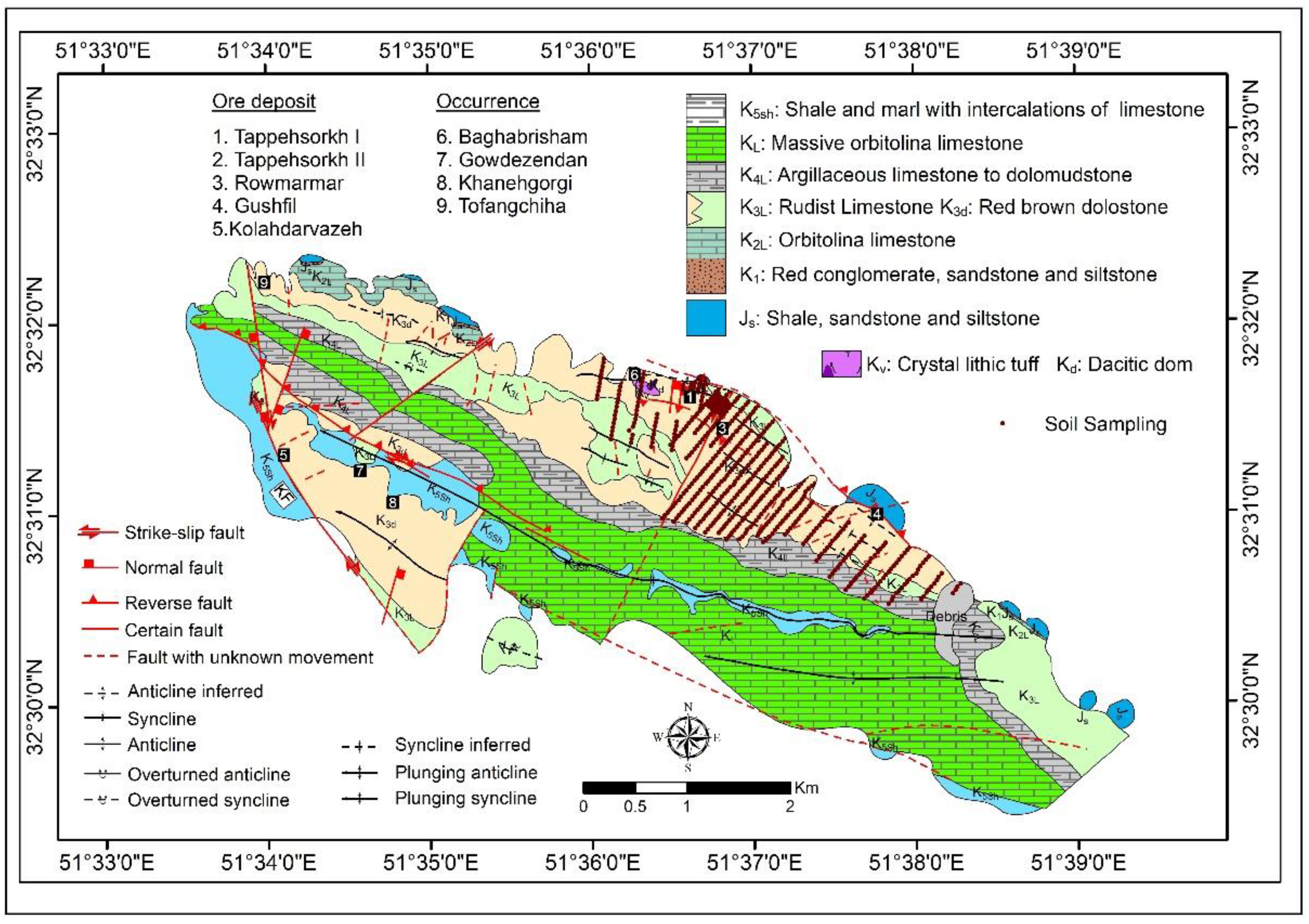
2. Geological Setting

The Irankuh Mining District (IMD) is one of the most important sediment-hosted Zn-Pb (Ag-Ba) deposits of Iran (Figure 1) formed within the back-arc extensional setting during the Late Jurassic-Lower Cretaceous Age of Sanandaj-Sirjan Zone (SSZ). SSZ is part of the NW-SE trending of the Zagros orogenic belt [57,58]. It is about 150–250 km wide, characterized by widespread Mesozoic volcanic and sedimentary rocks. The SSZ was a magmatic arc during the Jurassic Age. It then changed to a back-arc basin during the Early Cretaceous Age, where sedimentary rock units such as siltstone, sandstone, and carbonates were deposited in the resulted sedimentary basin. This sedimentary basin hosts about 170 Middle to Upper Jurassic [59] and Lower Cretaceous sediment-hosted [60] Zn-Pb deposits and occurrences constituting the Malayer-Esfahan Metallogenic Belt.

The IMD contains several economic deposits, such as Tappehsorkh, Gushfil, Rowmarmar, and Kolahdarvazeh, which are now active. Mineralization occurred as stratiform and stratabound bodies of sulfide and non-sulfide ores within Lower Cretaceous dolostone, siltstone, and crystal lithic tuff. Jurassic shale, sandstone, and siltstone are the oldest rocks unconformably covered by Lower Cretaceous volcano-sedimentary rock units. Volcanic rocks are dominated by crystal lithic tuff, andesitic rocks intersected by the dacitic dome. Lower Cretaceous sedimentary rocks include conglomerate, siltstone, dolostone, and limestone. One of the essential features in the IMD is the WNW-ESE trending Gushfil-Baghabrisham fault, which was common in the Lower Cretaceous (contemporaneous with the formation of a back-arc basin and sulfide deposition) but changed to reverse fault due to inversion tectonic of Late Cretaceous compression tectonism [61]. Based on [62,63,64], this fault is the main conduit controlling the movement of ore-bearing fluids that deposited economic stratiform and stratabound sulfide minerals in the proximal host rocks.

Based on the geology, tectonic setting, mineralogy, ore texture, geochemical, and isotopic analytical results, the IMD and included ore deposits have been classified as sub-seafloor diagenetic replacement SEDEX-type deposits [62,63,64]. Karimpour and Sadeghi [65,66], based on the deposition of sulfide minerals within or close to dolostone and shale-siltstone units and replacement and open space filling textures of ore minerals, suggested this deposit occurred as an MVT-type deposit. The Gushfil ore deposit was extracted as an open pit, but since 2006 it has been mined as underground. The Tappehsorkh deposit is mined as an open pit in Tappehsorkh I and Tappehsorkh II. Mining activities at the Kolahdarvazeh deposit are also carried out as open-pit activities. At the Rowmarmar deposit, the ore is extracted by underground activities within dolostone host rocks. All the deposits in IMD now have 13.9 Mt ore in total with an average grade of 0.95% Pb, 5.5% Zn, and 700 g/t Ag at the Gushfil deposit, 2.2% Pb, 4.3% Zn at Tappehsorkh deposit, 1.1% Pb, 9.9% Zn at Kolahdarvazeh deposit, and 1.55% Pb and 4.35% Zn at Rowmarmar deposit [67].

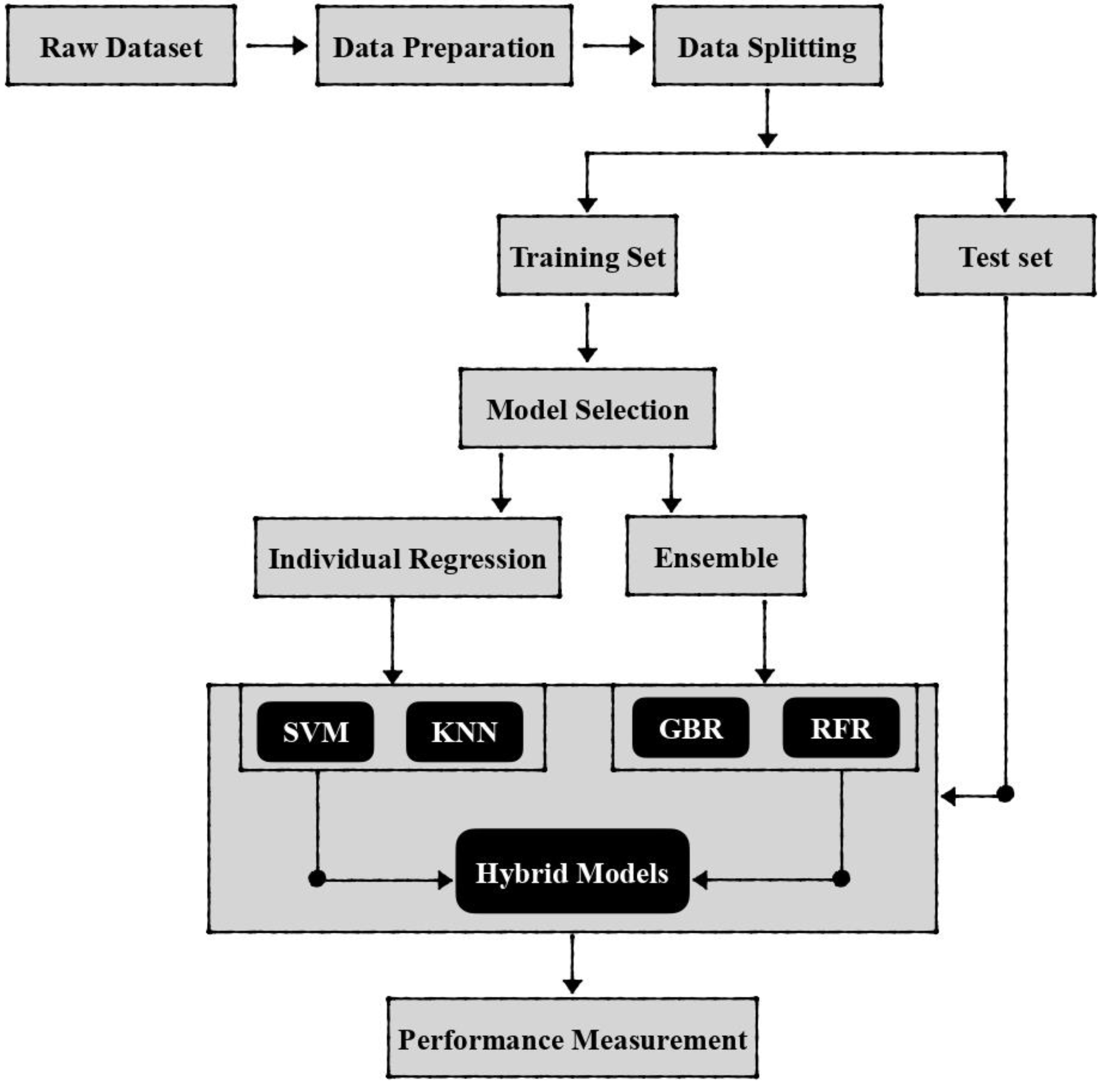
3. Material and Methods

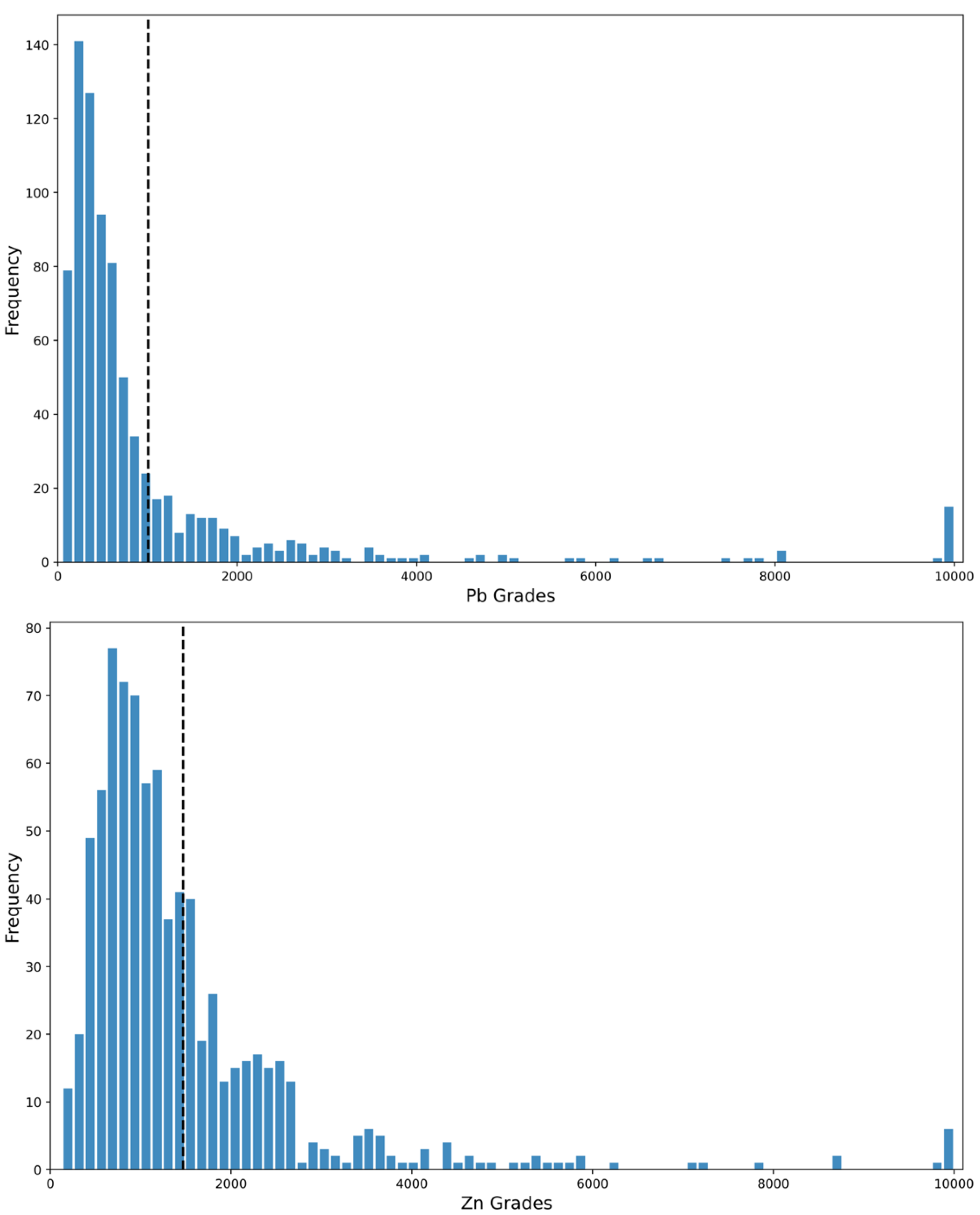
3.1. Dataset

All the models have been trained using Scikit-learn as one of the most common Python packages for ML algorithms [68]. For this study, the dataset compromised 804 in situ samples. A rectangular grid with about 40-m intervals and 200-m length has been designed at the northern part of IMD for Pb-Zn geochemical exploration. Then, 804 samples were selected from in situ soil samples in this grid for further geochemical analyses. Three to five samples located within the 5 to 10-m range were chosen as one individual specimen to send to the laboratory. All samples were taken from the B horizon at a depth varying from 20 to 30 cm to avoid the possible effects of contamination, such as mining activities or human pollution. The sampling lines were designed to intersect with the site, mining activities, mineralization zones, open pits, faults, fracture zones, and tailing sites. After sampling, all the samples were submitted to ALS Chemex in Canada for 35 elements analysis by ICP-MS conducting microwave digestion with a 1:1 nitric-hydrochloric acid mixture. The precision varied from ±0.1% to ±10% at the 95% confidence level. The statistical parameters summary of the datasets is shown in

Table 1. Statistical properties of Pb and Zn for all instances [unit: %].

Elements	Count	Mean	Std. 1	Minimum	25%	50%	75%	Maximum
Pb	804	0.01008	1672	0.0047	0.0279	0.0487	0.0912	1
Zn	804	0.147	1343	0.0134	0.0725	0.1092	0.1703	1

¹ Standard Deviation.

.

The histograms for Pb and Zn are represented in Figure 2. Both Pb and Zn grade values have positive skewness. Few spots are rich in Pb or Zn. In geochemical exploration, the determination of multiple cell dimensions within the 2D model is substantial. For this purpose, a general approach has been proposed for the operation according to the sampling models and ore deposit type. Accordingly, cell sizes are equal to 40 m × 40 m for X and Y, respectively [69].

Another step in geochemical exploration studies is outlier identification, an essential task in the statistical analysis of geochemical data, especially the separation of anomalies from the background. The outliers are the abnormal data that deviate from the usual data range. Outliers often are indications for mineral deposit explorations because high anomalies were shown [70]. Thus, recognition and decisions for correcting or removing them are significant during preprocessing data. Many methods have been proposed for the signification of the outlier data. The Dorffel method is used to distinguish the outlier data in which appropriate data replaced the outlier data.

3.2. K-Nearest Neighbor (KNN)

The KNN model is one of the most efficient and straightforward ML algorithms. This technique has been used in different regression and classification models ever since Cover and Hart [71] have proposed this method. The KNN model has some strengths, such as performing well without needing many adjustments; therefore, it can be a good baseline as it is an understandable method before employing advanced and complex techniques [72,73]. The main idea of this method is to use the neighborhood between the independent variable of the predictors and calculate this variable in the historical dataset to obtain the best estimators for the predictor [74]. The algorithm finds out the nearest neighbors’ point in the training dataset for the given dataset. Therefore, the KNN algorithm mainly depends on the distance and voting function of the selected optimal value of K [75].

For the KNN algorithm, a large and small k-value could result in overfitting and noise, respectively [76]. Therefore, the hyperparameters such as n-neighbor, leaf-size, and metrics have been adjusted to obtain the best performance of the KNN model in this study, and the optimal hyperparameters for this technique have been shown in (

Table 2. Optimal hyperparameters for the applied ML models.

Model	Hyperparameters	Model Parameters
KNN	N_neighbor	11
	Leaf_size	10
	Metric	‘Euclidean’
SVM	Kernel	‘sigmoid’
	Gamma	‘scale’
	C	1
GBR	N_estimator	500
	Max_depth	5
	Learning_rate	0.1
RFR	N_estimator	400
	Max_depth	10
	Max_features	log2

). The Chebyshev, Euclidean, Manhattan, and Minkowski have been tested for length metric. The Euclidean metric has shown the best result among other parameters. To find the optimal value for n-neighbor and leaf-size, the grid search method has been applied.

3.3. Support Vector Machine (SVM)

This technique has become a popular approach for solving classification, regression, and anomaly detection problems [77]. The methodology of the SVM has been proposed by Cortes and Vapnik [78]. The SVM method is designed for classification, and the sparse solution and reasonable generalization of SVM lend themselves to adaption to regression. The SVM is called support vector regression (SVR) for application in regression analysis [79]. The optimal value of kernel, gamma, and C (Table 2) for the SVR model was estimated through the grid method [80]. For more explanation about the SVM model, readers are referred to the literature [81,82].

3.4. Random Forest (RF)

The RF technique was initially introduced by Ho [83] and developed by Breiman [84] around twenty years ago. Currently, it is among the most popular existing supervised methods of ML research [85] and is very effective for most regression analyses. The method connects the concept of bagging, which was introduced by [84], and random feature selection, which was first proposed by [83]. The RF method is principally a gathering of multiple decision tree predictors, where each tree is unique and dissimilar to the others. The total number of predictors and trees are used to control the node split between the model, which affects the complexity of the model [86]. Because of building many trees, the results have been calculated as the average value of all the regression trees [79]. The aim of RF is to collect the computed results from different trees as a “weak learner” and build the algorithm; for this purpose, many decision trees are required. The other steps of random forest have been explained in detail by [87]. The random forest gets its name by implanting randomness in the trees to make sure each one of them is unique and different [37]. In addition, the rigorous mathematics relative to this technique can be found in [84,85,86,87,88].

This method has various advantages such as its use for both numerical and categorical datasets, adaptability to both regression and classification problems, and its capability of handling non-linear variables [89,90,91,92]. It does not require any specific assumptions for the statistical distribution of the data. Hyperparameters for this algorithm (Table 2) include n_estimator as the number of trees in the forest, max_features, which is splitting the nodes, and max_depth as the pre-pruning parameter [79,80,81,82,83,84,85,86,87,88,89,90,91]. As the other technique, the optimal hyperparameters have been obtained using the grid search method.

3.5. Gradient Boosting Regression (GBR)

The GBR is an efficient and accurate model, which can use for both regression and classification. In this technique, adding different trees is required to obtain an optimal model; however, weak generalization can occur when the model is trained too well on the input training data [93]. The error or residual can be defined as the loss function in the ML terminology [94]. The main framework of this technique is boosting, and the fundamental aim is minimizing the loss function. In the gradient boosting algorithm, different loss functions can be defined based on the problem [95,96]. The primary point of employing the GBR is its ability to use fewer computational resources for the objective function [93,94,95,96,97].

The steps involved in this algorithm are as follows [95,96,97,98]:

• A loss function is required, and it should be differentiable; therefore, the entire processing can be focused on minimizing this function.
• Generating the decision tree as the weak learner for predicting values.
• To add the weak learners and minimize the loss function, an addictive model is required.

In principle, the GBR model’s hyperparameters (Table 2) are identical to the RF model, which are n_estimator, max_depth, and learning_rate, and these are not present in the RF model [99]. A detailed mathematical explanation of this method for further study can be found in the related literature [100,101,102].

3.6. Hybrid Regression Models

This study developed two hybrid regression models SVM-KNN-RFR(SKR) and SVM-KNN-GBR(SKG) to improve the ore grade prediction. As indicated in the introduction, the individual regression methods are good and popular for ore grade predictions and mineral exploration. However, these techniques do not perform efficiently enough when the dataset is small [103]. Therefore, a hybrid model that combines both methods has been developed to overcome this obstacle and improve the model performance. The result of this hybrid model can be expressed as follows [79]:

$$\mathsf{\mu }\left(\mathrm{X}\right)=\frac{1}{\mathrm{N}}\sum _{\mathrm{n}=1}^{\mathrm{N}}{\mathsf{\omega }}_{\mathrm{n}}{\mathrm{P}}_{\mathrm{n}}\left(\mathrm{X}\right)$$

(1)

where $\mathsf{\mu }\left(\mathrm{X}\right)$ is the weighted average result of the model, ${\mathsf{\omega }}_{\mathrm{n}}$ is the weight assigned to the n^th regressor, ${\mathrm{P}}_{\mathrm{n}}\left(\mathrm{X}\right)$ is the prediction related to the n^th model, and X is the sample data. This hybrid model can enhance the results by controlling the variance considering the tiny dataset and avoiding the generalization error [104]. The workflow of the models is illustrated in Figure 3.

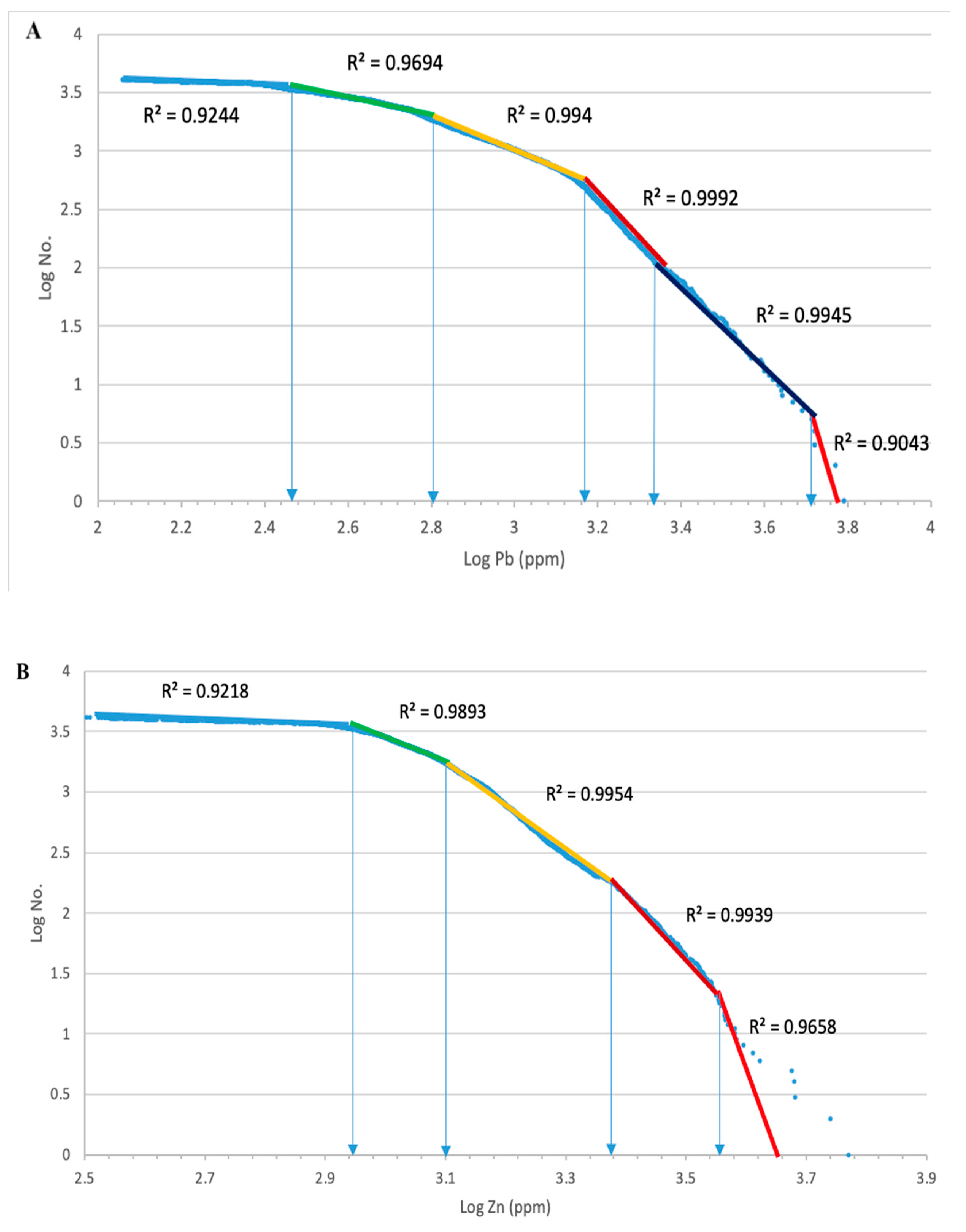
3.7. Concentration-Area (C-A) Fractal Method

The C-A is based on a reverse relationship between ore elemental concentrations and their occupied areas proposed by Cheng et al. (1994) for the first time [7]. This method has been used to interpret geochemical data and classify geochemical anomalies based on stream sediments, rock samples, and in situ soil samples [50,105,106]. This model is based on gridding interpolation data derived via geostatistical estimation/simulation. The C-A log-log plot is essential to define geochemical background and anomalies, and mineralized zones in different case studies. A reverse relationship between ore grades and their cumulative occupied areas can provide a better interpretation for geochemical populations [14,107,108]. Operation of this model is related to the interpolation model because it is essential and effective in detecting boundaries between different anomalies. General estimation methods such as (inverse distance weighted) IDW and kriging package are used for in situ rock and soil samples [109].

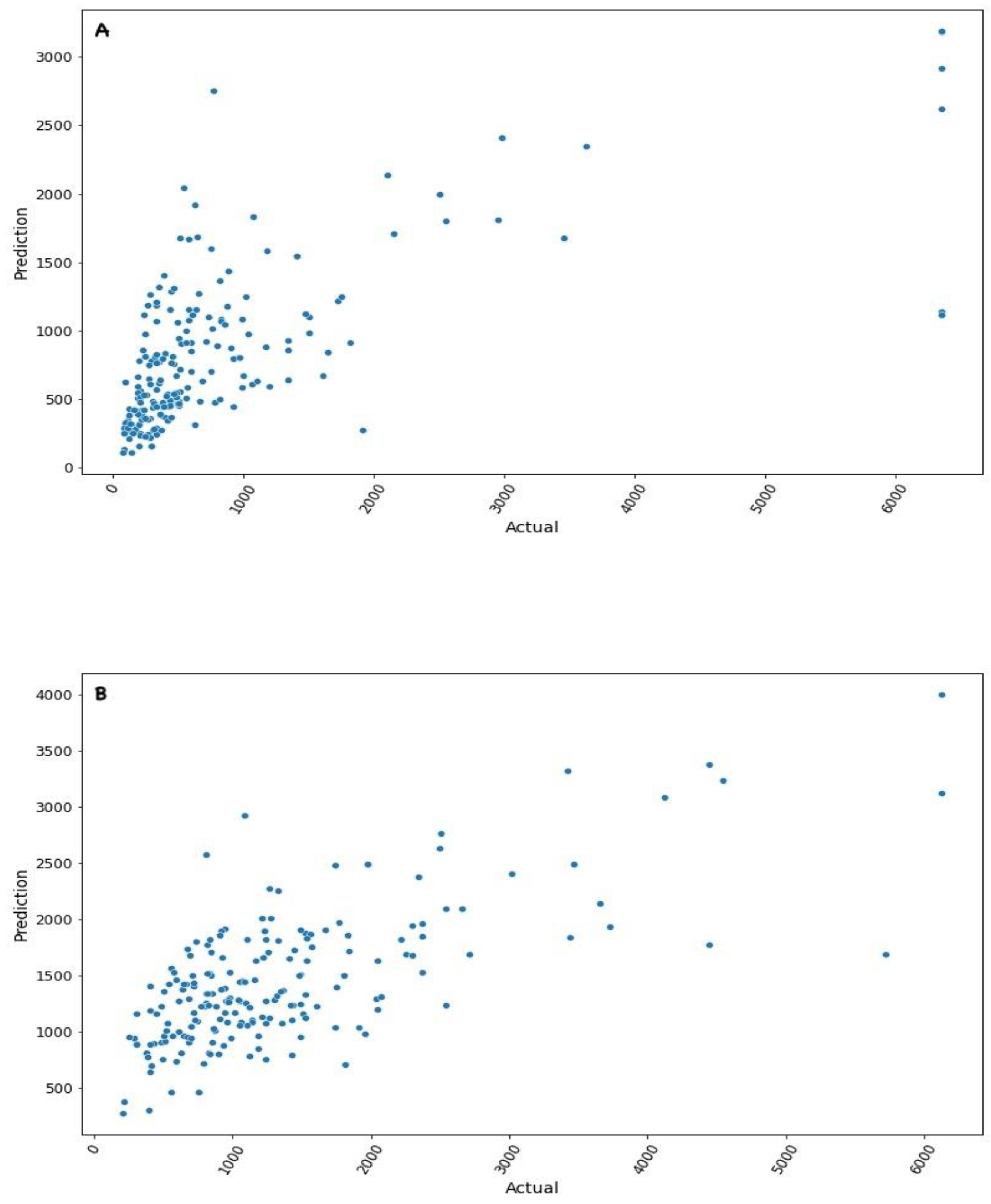
4. Results

The selected hyperparameters for each ML model are listed in Table 2. Moreover, the selected models have been compared by different metrics, including correlation coefficients, mean absolute error, and mean squared error, and the final results are shown in

Table 3. Comparison between estimated and raw data based on the ML models by correlation coefficient.

Elements	Metrics	KNN	SVM	GBR	RFR	Hybrid (SKG)	Hybrid (SKR)
Pb	Correlation Coefficient	+0.65%	+0.56%	+0.73%	+0.66	0.74	0.71
	Mean Absolute Error	607.10	508.30	395.20	580.70	338.90	380.10
	Mean Squared Error	1039.20	1130.80	766.80	992.40	754.70	760.50
Zn	Correlation Coefficient	+0.60	+0.45	+0.65	+0.62	+0.66	+0.63
	Mean Absolute Error	487.20	589.50	470.10	475.10	451.40	472.50
	Mean Squared Error	797.50	920.10	768.90	722.20	667.40	716.80

. The correlation plot for the SKG hybrid model for Pb and Zn is shown in Figure 4.

The C-A log-log plots, generated for Pb and Zn, are based on the results obtained by the SKG hybrid model, as depicted in Figure 5. There are five populations for Zn and Pb, and the multifractal nature exists in the output plots, and lastly, the anomaly distribution was all generated by GIS, as shown in Figure 6.

To show the relationship between the Pb and Zn data predicted by the machine learning method and the results of borehole studies, the two plot diagrams between these data have been drawn in the next step. For this reason, each borehole data is compared with the near cell predicted by the ML method (Figure 7). As observed, there are positive correlations, +0.34 and +0.46 for Pb and Zn, respectively. These results indicate a proper statistical validation for this methodology.

5. Discussion

5.1. Machine Learning

In total, 4116 cells were estimated by the final selected method. In this study, the two hybrid regression models have been built, and the outputs have been compared with four regression ML techniques. The ML models have been employed to predict the ore grade of Pb and Zn in the IMD, Central Iran. In this model, 80% of the data has been considered for the training and validation process, and the remaining 20% has been used for the model testing. Optimal hyperparameters are required to make an accurate and robust model, greatly depending on the specific dataset [110,111]. For this purpose, the k-fold (K-10) cross-validation methodology has been set in the proposed algorithms; thus, there are ten different training set portions [112]. Moreover, the performance of each model is computed on the testing dataset. To evaluate the performance of each model, means square error (MSE), mean absolute error (MAE), and the correlation coefficient were chosen.

The results demonstrate that the GBR has the most accurate outcomes among the individual regression models (Table 3). Both hybrid models outperform all other regression models and provide acceptable results. However, the SKG hybrid model depicts the best performance among all other models with the correlation coefficient values of 0.74 and 0.66 for Pb and Zn, respectively, as shown in Figure 4. Consequently, the results were derived via this hybrid model selected for fractal modeling. SVM has the worst performance among all the applied models, with the lowest correlation coefficient of 0.56 and 0.45 for Pb and Zn. In this study, four different ML regression and two hybrid models have been utilized to estimate the concentrations of Pb and Zn. The testing dataset has evaluated the performance of each model. Consequently, the predictive potential of the Hybrid regression models was examined, and the results were compared with the other models’ analysis based on the different metric values.

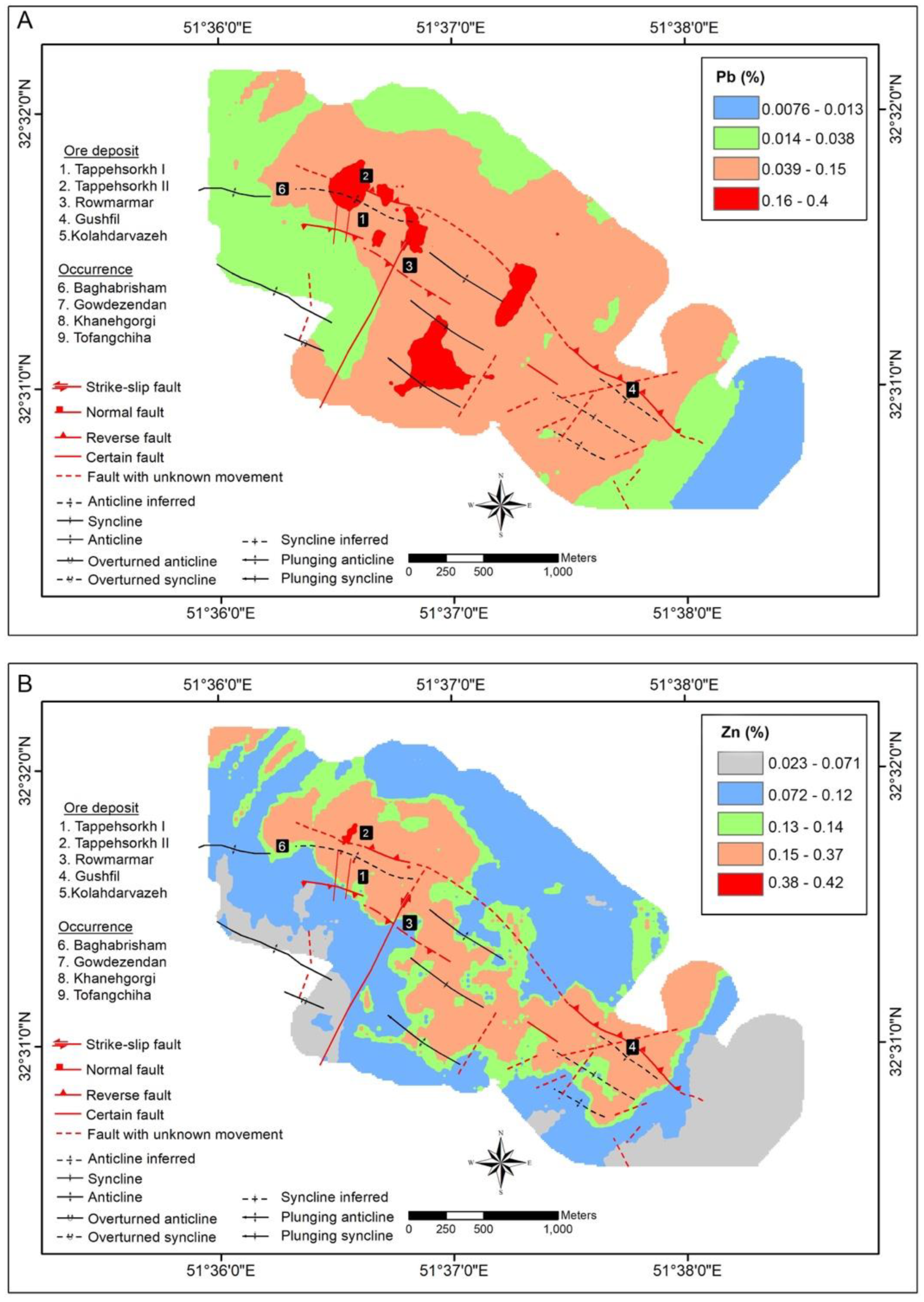
5.2. Fractal Modeling

The log-log plots (Figure 5) have been generated by the output results of the SKG hybrid model for both Pb and Zn. Based on the resulted fractal domains, the anomaly distribution maps of these elements were generated at GIS (Figure 6). The lowest Pb values vary from 0.0076 to 0.013 %, demonstrating the background population, as observed in Figure 6. Next populations have 0.014 to 0.038 % (upper background) and 0.039 to 0.15 % (third class anomaly), respectively. The highest Pb values with 0.16 to 0.4 % domain show the first-class anomaly in the IMD.

The Zn populations commence with 0.023 to 0.071 % for background values (Figure 6). It is followed by 0.072 to 0.12 % (upper background) and 0.13 to 0.14 % (third class anomaly). The next group ranges from 0.15 to 0.37 %, the second-class Zn anomaly. The highest Zn grades with 0.38 to 0.42 % are considered a first-class Zn anomaly at the IMD. Thus, it is concluded that the main Pb and Zn begin from 0.64% and 0.48%, respectively. Furthermore, backgrounds for Pb and Zn are lower than 0.013% and 0.0234%, correspondingly, based on these log-log plots. Major Pb anomalies occur in the north west, central and southern parts of this area (Figure 6). In addition, high extensive anomalous parts of Zn (First and second class) occur in the NW-SE trending at IMD (Figure 6).

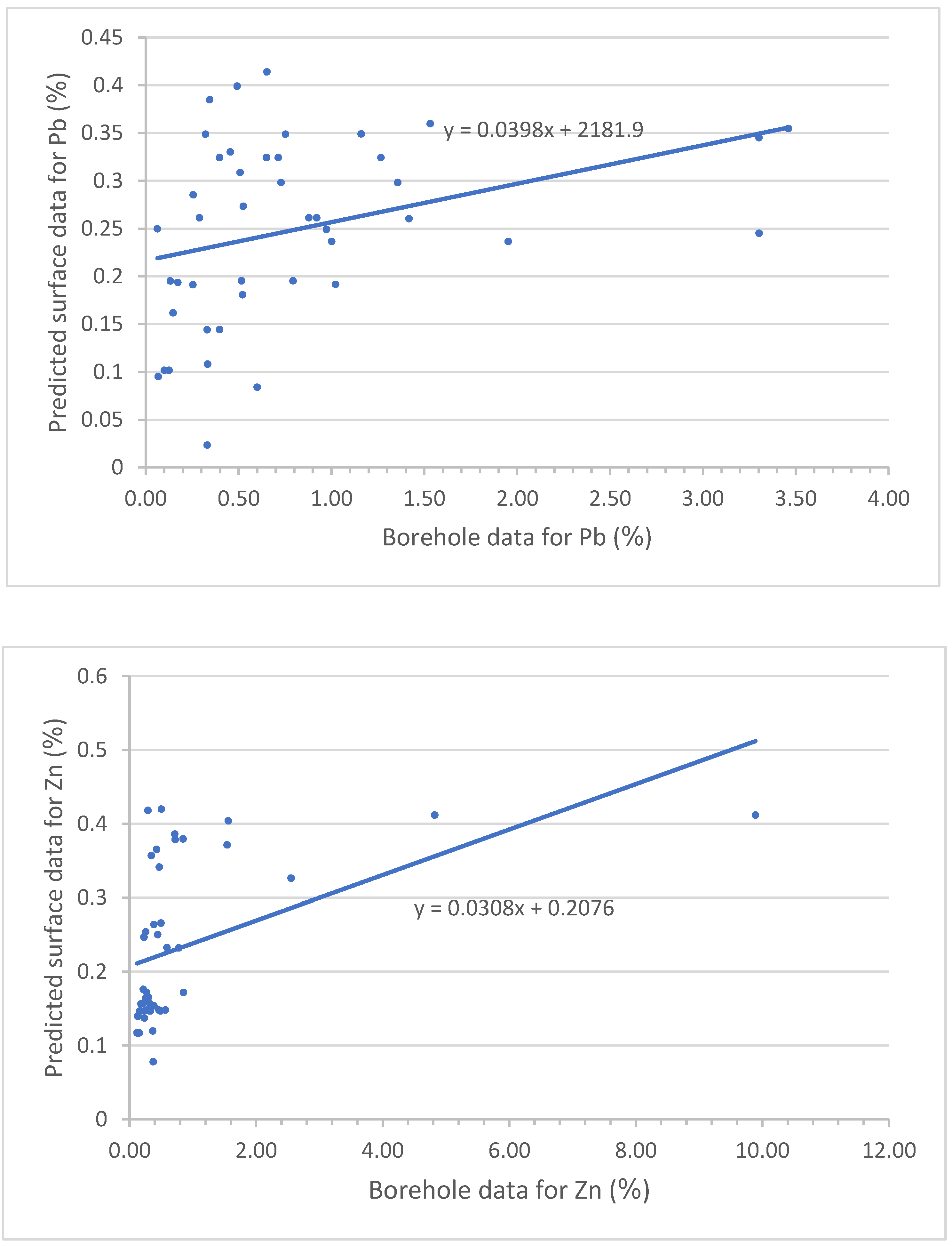
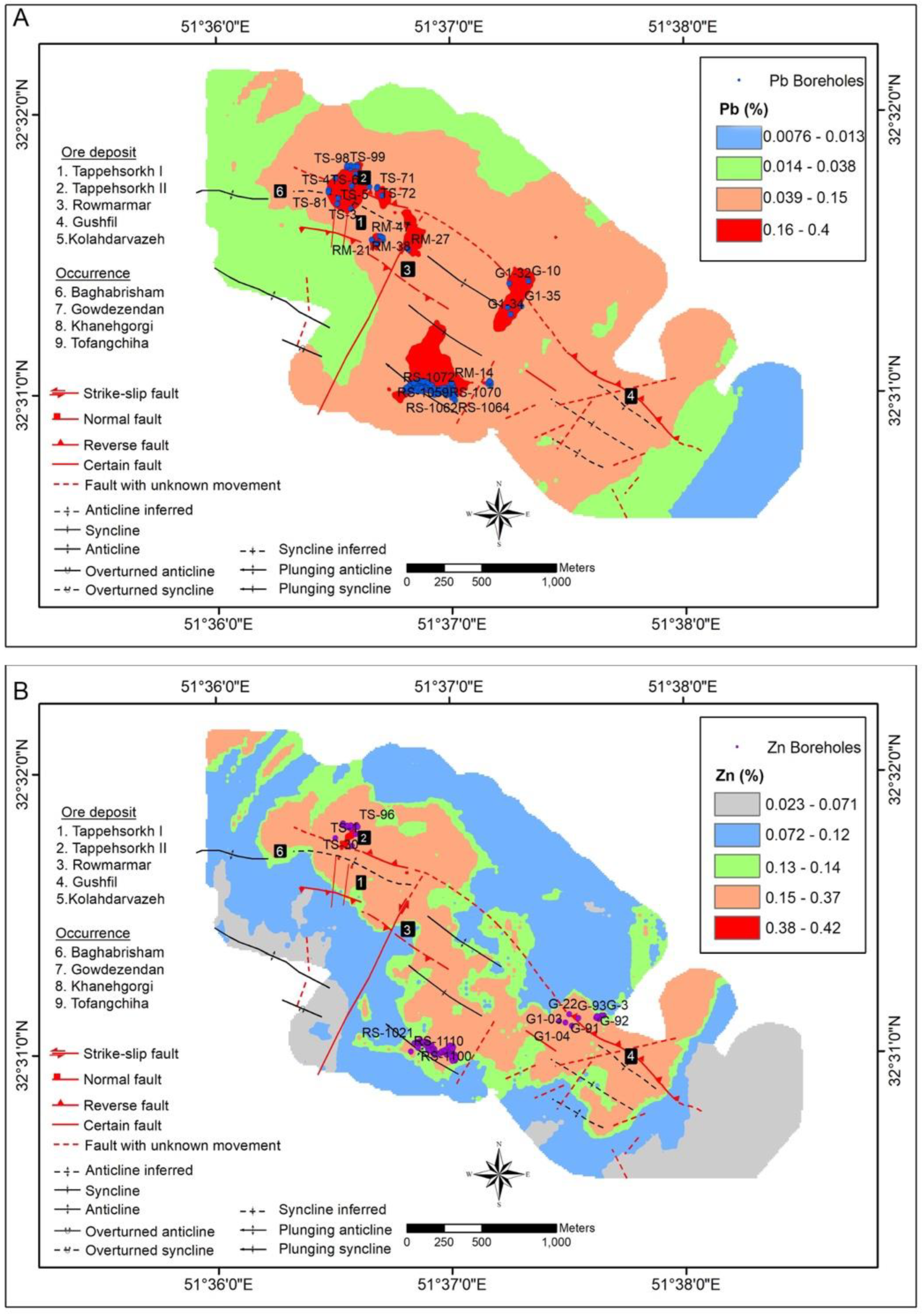
5.3. Validation by Core Drilling Data

The outputs were compared with mining activities’ location and borehole Pb-Zn averages to evaluate results derived via the ML and fractal methods. The Pb anomalies in the IMD are classified into four groups based on the values taken from the C-A fractal analysis (Figure 6). These results of Pb values could be considered a first-class anomaly (0.16–0.4 %). Pb anomalies are located on the sulfide orebodies from the Tappehsorkh deposit to the Rowmarmar deposit, which are now under mining, as depicted in Figure 6. One accumulation of Pb anomaly was placed in an area between Rowmarmar and Gushfil deposits, which could be essential for later exploration planning. It should be noted that the second class of Pb anomaly with about 0.039 to 0.15 % is also important due to the high values of Pb (greater than background values). This anomaly class is distributed at almost the whole area between mining exploration sites, which emphasizes that the amount of Pb is higher than the background grades in these regions. Zn concentrations are classified into five groups based on the fractal analysis. The first and second classes of anomalies are compiled with 0.38 to 0.42 % and 0.15 to 0.37 %, respectively. The Zn anomalies are well distributed where the Tappehsorkh, Rowmarmar and Gushfil deposits are getting mined now (Figure 8). Other Zn anomalies are located where whole deposits and occurrences formed. It is spatially extending among and around the mining site, which confirms high Zn distribution values in soil sampling from this area. It could also be due to Zn mobilization affinity in the rock unit and later redistribution. It is necessary to note that major anomalies of Pb and Zn are located in the regionally dolomitized K3l orbitolina limestone, which is called as the K3d dolostone unit (Figure 1).

There are many exploratory boreholes in the IMD investigating the trend of sulfide orebodies throughout the exploration area. As shown in Figure 8, some of them were drilled on the Pb and Zn anomalies resulting from the fractal analysis. Some of the drilled boreholes are well located at the first and second classes resulting in Zn and Pb anomalies. As demonstrated in

Table A1. Pb and Zn grades of boreholes correlated with the Pb fractal analysis results.

Row	BHs Name	Min		Max		Mean		Median
		Total Pb	Total Zn	Total Pb	Total Zn	Total Pb	Total Zn	Total Pb	Total Zn
1	G-10	0.00	0.02	0.10	1.50	0.05	0.14	0.06	0.02
2	RM14	0.04	0.08	9.80	1.77	0.77	0.72	0.38	0.67
3	RM15	0.02	0.06	13.60	13.00	0.56	1.63	0.12	0.79
4	RM16	0.02	0.05	10.00	9.00	0.12	0.39	0.12	0.39
5	RM17	0.02	0.07	31.00	8.10	2.70	1.00	0.16	0.32
6	RM18	0.02	0.06	7.24	33.00	0.41	2.50	0.14	1.26
7	RM19	0.02	0.07	12.00	30.00	0.43	1.77	0.12	0.55
8	RM21	0.02	0.08	6.00	23.50	0.24	1.42	0.08	0.55
9	RM27	0.02	0.02	0.16	0.15	0.10	0.08	0.11	0.07
10	RM29	0.02	0.06	14.60	8.10	0.38	0.73	0.10	0.41
11	RM38	0.04	0.06	24.00	6.50	0.98	0.54	0.20	0.29
12	RM47	0.02	0.03	18.00	8.00	0.36	0.65	0.04	0.36
13	TS1	0.02	0.02	1.36	22.50	0.13	0.85	0.04	0.17
14	TS3	0.04	0.02	22.00	18.50	1.82	1.73	0.36	0.38
15	TS4	0.02	0.05	50.00	11.00	2.97	1.07	0.40	0.40
16	TS5	0.04	0.02	35.00	24.25	0.30	0.63	0.30	0.63
17	TS6	0.02	0.02	12.40	21.20	0.63	0.81	0.10	0.20
18	TS21	0.02	0.05	1.88	18.50	0.24	1.11	0.14	0.50
19	TS23	0.02	0.05	18.40	3.40	0.33	0.34	0.08	0.21
20	TS26	0.02	0.07	5.70	5.25	0.51	0.47	0.14	0.20
21	TS28	0.04	0.04	2.60	12.50	0.16	0.64	0.04	0.11
22	TS29	0.02	0.03	4.10	1.50	0.25	0.38	0.04	0.27
23	TS30	0.04	0.04	5.70	3.50	0.97	0.45	0.16	0.18
24	TS37	0.02	0.05	26.00	8.00	0.62	0.88	0.12	0.25
25	TS59	0.08	0.05	25.60	10.50	6.55	0.85	2.24	0.20
26	TS60	0.04	0.02	0.52	1.01	0.15	0.15	0.08	0.04
27	TS63	0.08	0.02	46.10	2.93	9.49	0.35	0.70	0.08
28	TS65	0.04	0.07	0.16	0.44	0.08	0.21	0.08	0.16
29	TS70	0.02	0.03	14.80	16.35	0.61	0.69	0.04	0.08
30	TS71	0.08	0.05	0.20	0.50	0.11	0.24	0.09	0.16
31	TS72	0.02	0.03	22.00	5.50	0.99	0.83	0.12	0.20
32	TS80	0.04	0.07	35.60	2.00	2.57	0.64	0.14	0.61
33	TS81	0.04	0.04	23.60	1.52	2.03	0.51	0.10	0.30
34	TS96	0.02	0.19	0.16	1.15	0.06	0.59	0.04	0.53
35	TS97	0.02	0.01	17.00	21.00	0.40	1.54	0.04	0.12
36	TS98	0.02	0.03	26.00	2.35	1.42	0.29	0.04	0.16
37	TS99	0.02	0.02	4.44	8.90	0.52	0.72	0.06	0.15
38	TS101	0.14	0.12	11.20	35.60	3.30	9.89	2.45	5.35
39	TS102	0.02	0.04	18.40	22.00	3.30	4.82	1.72	0.97
40	TS103	0.02	0.01	5.60	9.15	0.33	0.78	0.04	0.11
41	TS104	0.02	0.01	20.40	5.50	1.02	0.43	0.08	0.19
42	G1-32	0.02	0.01	7.30	0.84	0.63	0.13	0.08	0.08
43	G1-33	0.01	0.01	3.04	6.85	0.12	0.35	0.02	0.08
44	G1-34	0.02	0.08	6.70	8.30	0.43	0.48	0.12	0.23
45	G1-35	0.02	0.01	1.34	4.30	0.26	0.20	0.16	0.15
46	RS-1012	0.02	0.09	6.68	1.59	1.27	0.33	0.18	0.21
47	RS-1013	0.06	0.02	1.34	1.95	0.33	0.38	0.14	0.13
48	RS-1014	0.14	0.08	4.50	1.75	0.92	0.57	0.31	0.33
49	RS-1015	0.02	0.08	1.56	0.68	0.29	0.28	0.16	0.27
50	RS-1016	0.02	0.08	6.34	1.65	0.88	0.47	0.20	0.26
51	RS-1017	0.24	0.10	9.00	0.68	1.95	0.31	1.50	0.30
52	RS-1018	0.04	0.04	5.10	0.41	1.00	0.16	0.66	0.14
53	RS-1019	0.02	0.08	5.00	0.44	0.65	0.18	0.16	0.16
54	RS-1020	0.10	0.03	4.40	0.70	0.75	0.25	0.40	0.21
55	RS-1021	0.02	0.03	0.38	0.41	0.13	0.12	0.12	0.09
56	RS-1022	0.02	0.06	0.46	0.66	0.07	0.15	0.04	0.11
57	RS-1023	0.02	0.03	1.86	0.96	0.35	0.26	0.14	0.19
58	RS-1024	0.02	0.04	0.22	0.42	0.10	0.13	0.06	0.08
59	RS-1025	0.02	0.09	2.40	0.91	0.26	0.30	0.07	0.23
60	RS-1026	0.10	0.06	2.12	0.54	0.33	0.22	0.16	0.14
61	RS-1027	0.06	0.17	2.44	1.27	0.32	0.38	0.14	0.31
62	RS-1028	0.04	0.08	2.70	2.30	0.49	0.50	0.12	0.29
63	RS-1029	0.02	0.09	3.76	0.77	0.40	0.23	0.10	0.16
64	RS-1030	0.08	0.16	11.00	2.50	1.36	0.85	0.79	0.69
65	RS-1031	0.02	0.10	4.28	0.81	0.73	0.27	0.14	0.21
66	RS-1032	0.10	0.15	3.90	1.10	0.71	0.49	0.20	0.49
67	RS-1033	0.04	0.15	3.46	0.36	0.53	0.23	0.28	0.22
68	RS-1034	0.08	0.05	4.40	0.60	0.52	0.18	0.20	0.13
69	RS-1035	0.02	0.11	10.20	0.95	0.79	0.33	0.20	0.27
70	RS-1036	0.02	0.11	1.86	0.69	0.17	0.34	0.04	0.36
71	RS-1037	0.02	0.09	1.28	0.95	0.15	0.22	0.06	0.15
72	RS-1038	0.02	0.11	3.12	2.49	0.65	0.72	0.18	0.63
73	RS-1039	0.06	0.10	4.06	1.68	0.46	0.50	0.22	0.32
74	RS-1040	0.06	0.09	2.44	2.77	0.44	0.67	0.26	0.39
75	RS-1041	0.08	0.17	3.46	1.50	0.59	0.45	0.30	0.35
76	RS-1042	0.02	0.10	1.66	0.86	0.25	0.28	0.10	0.21
77	RS-1043	0.02	0.08	0.60	0.83	0.15	0.26	0.14	0.15
78	RS-1044	0.10	0.23	1.24	0.54	0.53	0.36	0.28	0.28
79	RS-1045	0.06	0.23	5.40	1.76	0.87	0.62	0.56	0.59
80	RS-1046	0.02	0.18	0.32	2.00	0.15	1.04	0.16	1.20
81	RS-1047	0.02	0.20	1.40	1.80	0.20	0.49	0.12	0.41
82	RS-1048	0.02	0.11	4.00	0.90	0.81	0.38	0.30	0.34
83	RS-1049	0.02	0.03	0.40	0.62	0.13	0.16	0.08	0.15
84	RS-1050	0.30	0.36	12.80	0.91	3.48	0.66	1.44	0.75
85	RS-1051	0.02	0.06	1.08	0.65	0.21	0.26	0.08	0.17
86	RS-1052	0.02	0.07	2.72	1.41	0.55	0.32	0.08	0.21
87	RS-1053	0.02	0.05	0.52	0.42	0.10	0.16	0.04	0.13
88	RS-1054	0.02	0.04	1.34	0.91	0.18	0.21	0.04	0.16
89	RS-1055	0.06	0.07	1.60	0.88	0.48	0.36	0.35	0.25
90	RS-1056	0.02	0.10	0.36	0.70	0.08	0.20	0.04	0.13
91	RS-1057	0.02	0.02	0.16	0.45	0.05	0.12	0.04	0.09
92	RS-1058	0.02	0.02	0.10	0.61	0.05	0.16	0.04	0.15
93	RS-1059	0.02	0.03	0.30	0.28	0.09	0.11	0.06	0.08
94	RS-1060	0.02	0.05	0.84	0.28	0.08	0.14	0.04	0.13
95	RS-1062	0.08	0.21	2.00	1.15	0.39	0.57	0.22	0.49
96	RS-1063	0.02	0.13	1.56	1.57	0.23	0.44	0.10	0.34
97	RS-1064	0.02	0.05	0.72	1.16	0.11	0.36	0.06	0.32
98	RS-1069	0.02	0.04	2.16	0.93	0.25	0.24	0.04	0.16
99	RS-1070	0.02	0.05	0.48	2.22	0.12	0.34	0.06	0.11
100	RS-1071	0.02	0.07	3.04	1.50	0.30	0.29	0.14	0.23
101	RS-1072	0.02	0.07	3.04	1.50	0.30	0.29	0.14	0.23
102	RS-1074	0.02	0.03	0.52	0.83	0.15	0.24	0.10	0.21
103	RS-1075	0.02	0.07	0.68	2.00	0.16	0.39	0.08	0.23
104	RS-1081	0.12	0.05	4.76	0.73	0.60	0.27	0.32	0.20
105	RS-1085	0.08	0.05	2.14	0.51	0.74	0.27	0.70	0.25
106	RS-1086	0.12	0.05	0.60	0.42	0.25	0.22	0.23	0.22
107	RS-1087	0.08	0.14	2.00	0.52	0.61	0.29	0.46	0.30
108	RS-1088	0.04	0.07	1.52	0.55	0.33	0.26	0.18	0.26
109	RS-1089	0.10	0.12	0.90	0.57	0.49	0.32	0.47	0.35
110	RS-1090	0.02	0.09	1.70	0.46	0.19	0.26	0.10	0.24
111	RS-1091	0.20	0.30	1.14	0.70	0.45	0.43	0.37	0.37
112	RS-1092	0.02	0.09	3.32	0.63	0.48	0.21	1.00	0.38
113	RS-1093	0.10	0.22	1.72	0.55	0.43	0.34	0.28	0.32
114	RS-1094	0.06	0.11	2.96	0.54	0.54	0.23	0.25	0.21
115	RS-1095	0.10	0.13	1.60	0.65	0.58	0.35	0.56	0.30
116	RS-1096	0.04	0.11	1.96	0.56	0.48	0.32	0.40	0.31
117	RS-1097	0.08	0.11	1.16	0.66	0.44	0.30	0.37	0.29
118	RS-1098	0.06	0.08	1.72	0.61	0.45	0.33	0.48	0.31
119	RS-1099	0.04	0.30	0.44	0.45	0.25	0.37	0.26	0.37
120	RS-1100	0.16	0.20	4.06	0.81	1.16	0.37	0.84	0.32
121	RS-1101	0.16	0.16	0.72	0.57	0.36	0.31	0.32	0.29
122	RS-1102	0.10	0.17	0.88	0.43	0.34	0.28	0.30	0.27
123	RS-1103	0.02	0.08	0.16	0.47	0.05	0.25	0.04	0.24
124	RS-1104	0.16	0.10	1.24	0.45	0.47	0.29	0.40	0.28
125	RS-1105	0.02	0.18	0.58	0.63	0.26	0.33	0.26	0.32
126	RS-1107	0.02	0.07	0.16	0.70	0.07	0.15	0.08	0.11
127	RS-1108	0.02	0.10	0.08	0.33	0.04	0.19	0.04	0.17
128	RS-1109	0.02	0.07	1.06	0.92	0.15	0.25	0.04	0.22
129	RS-1110	0.08	0.07	1.06	0.38	0.60	0.24	0.64	0.27
130	RS-1112	0.02	0.07	0.16	0.32	0.06	0.15	0.06	0.14
131	RS-1114	0.10	0.02	0.48	0.26	0.27	0.12	0.28	0.10
132	RS-1116	0.06	0.08	1.08	0.36	0.22	0.18	0.14	0.19
133	RS-1118	0.06	0.02	0.96	0.41	0.28	0.16	0.15	0.16
134	RS-1120	0.04	0.01	1.64	0.67	0.25	0.22	0.12	0.23
135	RS-1122	0.12	0.02	2.56	0.46	0.62	0.20	0.36	0.23
136	RS-1163	0.02	0.08	6.88	1.41	0.61	0.46	0.22	0.44
137	RS-1166	0.08	0.39	1.40	0.85	0.37	0.69	0.24	0.70
138	RS-1177	0.02	0.13	1.04	1.22	0.34	0.67	0.20	0.61
139	RS-1179	0.02	0.15	0.60	1.18	0.20	0.48	0.18	0.42
140	RS-1181	0.02	0.04	0.50	0.96	0.16	0.23	0.10	0.17

Pb has an average of 0.03 to 9.48% in Pb fractal anomaly domains, whereas the Zn average ranged from 0.07 to 9.89% in this domain. Maximum values of Pb and Zn in this anomaly are about 50% in the TS04 borehole and 35.6% in the TS101 borehole (Table A1). The mean values of Pb and Zn located in the Zn anomaly area are about 0.045 to 4.48% and 0.1 to 9.89%, respectively (

Table A2. Pb and Zn grades of boreholes correlated based on the Zn fractal analysis results.

Row	BHs Name	Min		Max		Mean		Median
		Total Pb	Total Zn	Total Pb	Total Zn	Total Pb	Total Zn	Total Pb	Total Zn
1	TS1	0.02	0.02	1.36	22.50	0.13	0.85	0.04	0.17
2	TS26	0.02	0.07	5.70	5.25	0.51	0.47	0.14	0.20
3	TS29	0.02	0.03	4.10	1.50	0.25	0.38	0.04	0.27
4	TS30	0.04	0.04	5.70	3.50	0.97	0.45	0.16	0.18
5	TS96	0.02	0.19	0.16	1.15	0.06	0.59	0.04	0.53
6	TS97	0.02	0.01	17.00	21.00	0.40	1.54	0.04	0.12
7	TS98	0.02	0.03	26.00	2.35	1.42	0.29	0.04	0.16
8	TS99	0.02	0.02	4.44	8.90	0.52	0.72	0.06	0.15
9	TS100	0.02	0.01	40.60	32.70	3.46	1.56	0.10	0.12
10	TS101	0.14	0.12	11.20	35.60	3.30	9.89	2.45	5.35
11	TS102	0.02	0.04	18.40	22.00	3.30	4.82	1.72	0.97
12	TS103	0.02	0.01	5.60	9.15	0.33	0.78	0.04	0.11
13	TS104	0.02	0.01	20.40	5.50	1.02	0.43	0.08	0.19
14	TS105	0.02	0.05	28.80	26.00	1.53	2.55	0.15	0.38
15	G1-01	0.02	0.05	2.00	14.00	0.35	1.86	0.20	1.27
16	G1-03	0.01	0.10	1.00	20.75	0.12	1.00	0.08	0.60
17	G1-04	0.02	0.11	1.56	1.87	0.17	0.77	0.12	0.69
18	G1-07	0.06	0.19	2.16	23.30	0.35	3.15	0.16	1.48
19	G3	0.01	0.10	1.00	20.75	0.12	1.00	0.08	0.60
20	G22	0.04	0.06	6.72	32.00	0.66	2.41	0.26	1.22
21	G37	0.01	0.01	30.00	3.75	4.48	1.90	2.25	2.70
22	G67	0.04	0.10	3.70	12.50	0.50	2.38	0.20	0.90
23	G68	0.01	0.01	1.60	3.50	0.08	0.37	0.04	0.25
24	G88	0.01	0.01	3.60	19.40	0.55	3.70	0.21	1.07
25	G89	0.01	0.01	13.20	22.40	1.45	4.31	0.16	0.82
26	G90	0.01	0.01	0.10	0.80	0.05	0.25	0.04	0.10
27	G91	0.08	0.37	19.00	23.30	3.40	7.53	1.50	2.76
28	G92	0.02	0.08	6.60	13.70	0.80	3.27	0.08	0.95
29	G93	0.01	0.01	4.96	15.60	1.01	3.69	0.40	2.23
30	RS-1012	0.02	0.09	6.68	1.59	1.27	0.33	0.18	0.21
31	RS-1013	0.06	0.02	1.34	1.95	0.33	0.38	0.14	0.13
32	RS-1014	0.14	0.08	4.50	1.75	0.92	0.57	0.31	0.33
33	RS-1015	0.02	0.08	1.56	0.68	0.29	0.28	0.16	0.27
34	RS-1016	0.02	0.08	6.34	1.65	0.88	0.47	0.20	0.26
35	RS-1017	0.24	0.10	9.00	0.68	1.95	0.31	1.50	0.30
36	RS-1018	0.04	0.04	5.10	0.41	1.00	0.16	0.66	0.14
37	RS-1019	0.02	0.08	5.00	0.44	0.65	0.18	0.16	0.16
38	RS-1020	0.10	0.03	4.40	0.70	0.75	0.25	0.40	0.21
39	RS-1021	0.02	0.03	0.38	0.41	0.13	0.12	0.12	0.09
40	RS-1022	0.02	0.06	0.46	0.66	0.07	0.15	0.04	0.11
41	RS-1023	0.02	0.03	1.86	0.96	0.35	0.26	0.14	0.19
42	RS-1024	0.02	0.04	0.22	0.42	0.10	0.13	0.06	0.08
43	RS-1025	0.02	0.09	2.40	0.91	0.26	0.30	0.07	0.23
44	RS-1026	0.10	0.06	2.12	0.54	0.33	0.22	0.16	0.14
45	RS-1027	0.06	0.17	2.44	1.27	0.32	0.38	0.14	0.31
46	RS-1028	0.04	0.08	2.70	2.30	0.49	0.50	0.12	0.29
47	RS-1029	0.02	0.09	3.76	0.77	0.40	0.23	0.10	0.16
48	RS-1030	0.08	0.16	11.00	2.50	1.36	0.85	0.79	0.69
49	RS-1031	0.02	0.10	4.28	0.81	0.73	0.27	0.14	0.21
50	RS-1032	0.10	0.15	3.90	1.10	0.71	0.49	0.20	0.49
51	RS-1033	0.04	0.15	3.46	0.36	0.53	0.23	0.28	0.22
52	RS-1034	0.08	0.05	4.40	0.60	0.52	0.18	0.20	0.13
53	RS-1035	0.02	0.11	10.20	0.95	0.79	0.33	0.20	0.27
54	RS-1036	0.02	0.11	1.86	0.69	0.17	0.34	0.04	0.36
55	RS-1037	0.02	0.09	1.28	0.95	0.15	0.22	0.06	0.15
56	RS-1038	0.02	0.11	3.12	2.49	0.65	0.72	0.18	0.63
57	RS-1039	0.06	0.10	4.06	1.68	0.46	0.50	0.22	0.32
58	RS-1040	0.06	0.09	2.44	2.77	0.44	0.67	0.26	0.39
59	RS-1041	0.08	0.17	3.46	1.50	0.59	0.45	0.30	0.35
60	RS-1042	0.02	0.10	1.66	0.86	0.25	0.28	0.10	0.21
61	RS-1043	0.02	0.08	0.60	0.83	0.15	0.26	0.14	0.15
62	RS-1044	0.10	0.23	1.24	0.54	0.53	0.36	0.28	0.28
63	RS-1045	0.06	0.23	5.40	1.76	0.87	0.62	0.56	0.59
64	RS-1046	0.02	0.18	0.32	2.00	0.15	1.04	0.16	1.20
65	RS-1047	0.02	0.20	1.40	1.80	0.20	0.49	0.12	0.41
66	RS-1048	0.02	0.11	4.00	0.90	0.81	0.38	0.30	0.34
67	RS-1049	0.02	0.03	0.40	0.62	0.13	0.16	0.08	0.15
68	RS-1050	0.30	0.36	12.80	0.91	3.48	0.66	1.44	0.75
69	RS-1051	0.02	0.06	1.08	0.65	0.21	0.26	0.08	0.17
70	RS-1052	0.02	0.07	2.72	1.41	0.55	0.32	0.08	0.21
71	RS-1053	0.02	0.05	0.52	0.42	0.10	0.16	0.04	0.13
72	RS-1054	0.02	0.04	1.34	0.91	0.18	0.21	0.04	0.16
73	RS-1055	0.06	0.07	1.60	0.88	0.48	0.36	0.35	0.25
74	RS-1056	0.02	0.10	0.36	0.70	0.08	0.20	0.04	0.13
75	RS-1057	0.02	0.02	0.16	0.45	0.05	0.12	0.04	0.09
76	RS-1058	0.02	0.02	0.10	0.61	0.05	0.16	0.04	0.15
77	RS-1059	0.02	0.03	0.30	0.28	0.09	0.11	0.06	0.08
78	RS-1060	0.02	0.05	0.84	0.28	0.08	0.14	0.04	0.13
79	RS-1061	0.10	0.08	1.30	0.80	0.43	0.35	0.32	0.25
80	RS-1062	0.08	0.21	2.00	1.15	0.39	0.57	0.22	0.49
81	RS-1063	0.02	0.13	1.56	1.57	0.23	0.44	0.10	0.34
82	RS-1064	0.02	0.05	0.72	1.16	0.11	0.36	0.06	0.32
83	RS-1065	0.02	0.03	0.60	0.50	0.06	0.21	0.02	0.20
84	RS-1066	0.04	0.04	0.60	1.46	0.16	0.37	0.12	0.25
85	RS-1067	0.02	0.07	1.70	0.94	0.23	0.22	0.08	0.18
86	RS-1068	0.04	0.06	0.80	1.22	0.18	0.34	0.12	0.24
87	RS-1069	0.02	0.04	2.16	0.93	0.25	0.24	0.04	0.16
88	RS-1070	0.02	0.05	0.48	2.22	0.12	0.34	0.06	0.11
89	RS-1100	0.16	0.20	4.06	0.81	1.16	0.37	0.84	0.32
90	RS-1110	0.08	0.07	1.06	0.38	0.60	0.24	0.64	0.27

). The highest amount of Pb is about 40.6 % in the TS-100 borehole, and the highest value of Zn is about 35.6% in the TS-101 borehole (Table A2). Based on this correlation, the highest Pb and Zn grades are developed on the highest degrees of Pb and Zn anomaly resulting from the fractal analysis. Based on this correlation, it could be concluded that other Pb and Zn anomalies derived from fractal analysis, and especially those located between the Rowmarmar and Gushfil and Gushfil-e-Bala mining areas (Figure 8) could be suggested as prospects for detailed exploration in the IMD.

6. Conclusions

Precise grade estimation is substantial in geochemical exploration projects, affecting decision-making progress. In the present study, the analysis is carried out to determine if the combination of regression and ensemble models can improve the performance to build a more precise ore grade estimation. Therefore, two hybrid approaches (SKG and SKR) have been introduced. Three metrics have been selected to evaluate models, including correlation coefficients, MAE, and MSE. Although the introduced regression algorithms can solve problems as single, non-complex, and robust regression models, the hybrid technique can be used for the ore grade estimation with better performance. Our proposed hybrid regression model performed as the best ML model among all other introduced regression and ensemble models. The results are used to classify Pb and Zn anomalies by the C-A fractal model. This hybrid model based on ML and fractal modeling can be used in many geochemical exploration cases especially based on in situ rock and soil samples. In this case, a combination of fractal analysis of soil samples (surface sampling) and boreholes samples correlates with the location of mining activities in IMD. It could also have proposed potential targets for further exploration in future specially at the location between Rowmaramr and Gushfil mines (Figure 6 and Figure 8). The ML methods can be prepared suitable input for fractal models, especially the C-A fractal model. Considering the potential of ML techniques, integrating these methods and geostatistical simulation would be interesting for future research with more available data.

References

- Jafrasteh, B.; Fathianpour, N.; Suárez, A. Comparison of machine learning methods for copper ore grade estimation. Comput. Geosci. 2018, 22, 1371–1388. [Google Scholar] [CrossRef]
- Sinclair, A.J. Selection of threshold values in geochemical data using probability graphs. J. Geochem. Explor. 1974, 3, 129–149. [Google Scholar] [CrossRef]
- Sinclair, A.J. A fundamental approach to threshold estimation in exploration geochemistry: Probability plots revisited. J. Geochem. Explor. 1991, 41, 1–22. [Google Scholar] [CrossRef]
- Cheng, Q.; Agterberg, F.P.; Bonham-Carter, G.F. A spatial analysis method for geochemical anomaly separation. J. Geochem. Explor. 1996, 56, 183–195. [Google Scholar] [CrossRef]
- Zhang, C.; Manheim, F.T.; Hinde, J.; Grossman, J.N. Statistical characterization of a large geochemical database and effect of sample size. Appl. Geochem. 2005, 20, 1857–1874. [Google Scholar] [CrossRef]
- Luz, F.; Mateus, A.; Matos, J.X.; Gonçalves, M.A. Cu- and Zn-Soil Anomalies in the NE Border of the South Portuguese Zone (Iberian Variscides, Portugal) Identified by Multifractal and Geostatistical Analyses. Nat. Resour. Res. 2014, 23, 195–215. [Google Scholar] [CrossRef] [Green Version]
- Cheng, Q.; Agterberg, F.P.; Ballantyne, S.B. The separation of geochemical anomalies from background by fractal methods. J. Geochem. Explor. 1994, 51, 109–130. [Google Scholar] [CrossRef]
- Agterberg, F.P. Multifractal Modeling of the Sizes and Grades of Giant and Supergiant Deposits. Int. Geol. Rev. 1995, 37, 1–8. [Google Scholar] [CrossRef]
- Zuo, R.; Cheng, Q.; Xia, Q. Application of fractal models to characterization of vertical distribution of geochemical element concentration. J. Geochem. Explor. 2009, 102, 37–43. [Google Scholar] [CrossRef]
- Zuo, R.; Wang, J. Fractal/multifractal modeling of geochemical data: A review. J. Geochem. Explor. 2016, 164, 33–41. [Google Scholar] [CrossRef]
- Shahbazi, S.; Ghaderi, M.; Afzal, P. Prognosis of of gold mineralization phases by multifractal modeling in the Zehabad epithermal deposit NW Iran. Iran. J. Earth Sci. 2021, 13, 31–40. [Google Scholar] [CrossRef]
- Heidari, S.M.; Afzal, P.; Ghaderi, M.; Sadeghi, B. Detection of mineralization stages using zonality and multifractal modeling based on geological and geochemical data in the Au-(Cu) intrusion-related Gouzal-Bolagh deposit, NW Iran. Ore Geol. Rev. 2021, 139, 104561. [Google Scholar] [CrossRef]
- Sadeghi, B. Simulated-multifractal models: A futuristic review of multifractal modeling in geochemical anomaly classification. Ore Geol. Rev. 2021, 139, 104511. [Google Scholar] [CrossRef]
- Sadeghi, B.; Cohen, D.R. Category-based fractal modelling: A novel model to integrate the geology into the data for more effective processing and interpretation. J. Geochem. Explor. 2021, 226, 106783. [Google Scholar] [CrossRef]
- Sadeghi, B.; Cohen, D.R. Concentration-distance from centroids (C-DC) multifractal modeling: A novel approach to characterizing geochemical patterns based on sample distance from mineralization. Ore Geol. Rev. 2021, 137, 104302. [Google Scholar] [CrossRef]
- Zissimos, A.M.; Cohen, D.R.; Christoforou, I.C.; Sadeghi, B.; Rutherford, N.F. Controls on soil geochemistry fractal characteristics in Lemesos (Limassol), Cyprus. J. Geochem. Explor. 2021, 220, 106682. [Google Scholar] [CrossRef]
- Zuo, R.; Carranza, E.J.M.; Wang, J. Spatial analysis and visualization of exploration geochemical data. Earth-Sci. Rev. 2016, 158, 9–18. [Google Scholar] [CrossRef]
- Yu, X.; Xiao, F.; Zhou, Y.; Wang, Y.; Wang, K. Application of hierarchical clustering, singularity mapping, and Kohonen neural network to identify Ag-Au-Pb-Zn polymetallic mineralization associated geochemical anomaly in Pangxidong district. J. Geochem. Explor. 2019, 203, 87–95. [Google Scholar] [CrossRef]
- Xiao, F.; Chen, W.; Wang, J.; Erten, O. A Hybrid Logistic Regression: Gene Expression Programming Model and Its Application to Mineral Prospectivity Mapping. Nat. Resour. Res. 2021, 1–24. [Google Scholar] [CrossRef]
- Wang, H.; Yuan, Z.; Cheng, Q.; Zhang, S.; Sadeghi, B. Geochemical anomaly definition using stream sediments landscape modeling. Ore Geol. Rev. 2022, 142, 104715. [Google Scholar] [CrossRef]
- Zuo, R.; Xiong, Y.; Wang, J.; Carranza, E.J.M. Deep learning and its application in geochemical mapping. Earth-Sci. Rev. 2019, 192, 1–14. [Google Scholar] [CrossRef]
- Gonbadi, A.M.; Tabatabaei, S.H.; Carranza, E.J.M. Supervised geochemical anomaly detection by pattern recognition. J. Geochem. Explor. 2015, 157, 81–91. [Google Scholar] [CrossRef]
- Pati, Y.C.; Rezaiifar, R.; Krishnaprasad, P.S. Orthogonal matching pursuit: Recursive function approximation with applications to wavelet decomposition. In Proceedings of the 27th Asilomar Conference on Signals, Systems and Computers, Pacific Grove, CA, USA, 1–3 November 1993; IEEE Comput. Soc. Press: Pacific Grove, CA, USA, 1993; pp. 40–44. [Google Scholar] [CrossRef] [Green Version]
- Zhao, J.; Chen, S.; Zuo, R. Identifying geochemical anomalies associated with Au–Cu mineralization using multifractal and artificial neural network models in the Ningqiang district, Shaanxi, China. J. Geochem. Explor. 2016, 164, 54–64. [Google Scholar] [CrossRef]
- Zaremotlagh, S.; Hezarkhani, A. The use of decision tree induction and artificial neural networks for recognizing the geochemical distribution patterns of LREE in the Choghart deposit, Central Iran. J. Afr. Earth Sci. 2017, 128, 37–46. [Google Scholar] [CrossRef]
- Zhang, C.; Zuo, R.; Xiong, Y. Detection of the multivariate geochemical anomalies associated with mineralization using a deep convolutional neural network and a pixel-pair feature method. Appl. Geochem. 2021, 130, 104994. [Google Scholar] [CrossRef]
- Chen, Y.; Zhao, Q.; Lu, L. Combining the outputs of various k-nearest neighbor anomaly detectors to form a robust ensemble model for high-dimensional geochemical anomaly detection. J. Geochem. Explor. 2021, 231, 106875. [Google Scholar] [CrossRef]
- Saljoughi, B.S. A comparative analysis of artificial neural network (ANN), wavelet neural network (WNN), and support vector machine (SVM) data-driven models to mineral potential mapping for copper mineralizations in the Shahr-e-Babak region, Kerman, Iran. Appl. Geomat. 2018, 28, 229–256. [Google Scholar] [CrossRef]
- Li, T.; Zuo, R.; Xiong, Y.; Peng, Y. Random-Drop Data Augmentation of Deep Convolutional Neural Network for Mineral Prospectivity Mapping. Nat. Resour. Res. 2020, 30, 27–38. [Google Scholar] [CrossRef]
- Wang, J.; Zuo, R.; Xiong, Y. Mapping Mineral Prospectivity via Semi-supervised Random Forest. Nat. Resour. Res. 2020, 29, 189–202. [Google Scholar] [CrossRef]
- Wang, Z.; Zuo, R.; Jing, L. Fusion of Geochemical and Remote-Sensing Data for Lithological Mapping Using Random Forest Metric Learning. Math. Geosci. 2020, 53, 1125–1145. [Google Scholar] [CrossRef]
- Zhang, S.; Carranza, E.J.M.; Xiao, K.; Wei, H.; Yang, F.; Chen, Z.; Li, N.; Xiang, J. Mineral Prospectivity Mapping based on Isolation Forest and Random Forest: Implication for the Existence of Spatial Signature of Mineralization in Outliers. Nat. Resour. Res. 2021, 1–19. [Google Scholar] [CrossRef]
- Ibrahim, B.; Majeed, F.; Ewusi, A.; Ahenkorah, I. Residual geochemical gold grade prediction using extreme gradient boosting. Environ. Chall. 2022, 6, 100421. [Google Scholar] [CrossRef]
- Bédard, É.; De Bronac de Vazelhes, V.; Beaudoin, G. Performance of predictive supervised classification models of trace elements in magnetite for mineral exploration. J. Geochem. Explor. 2022, 236, 106959. [Google Scholar] [CrossRef]
- Kaplan, U.E.; Topal, E. A New Ore Grade Estimation Using Combine Machine Learning Algorithms. Minerals 2020, 10, 847. [Google Scholar] [CrossRef]
- Jordan, M.I.; Mitchell, T.M. Machine learning: Trends, perspectives, and prospects. Science 2015, 349, 255–260. [Google Scholar] [CrossRef] [PubMed]
- Muller, A.C.; Guido, S. Introduction to Machine Learning with Python: A Guide for Data Scientists; O’Reilly Media, Inc.: Newton, MA, USA, 2016. [Google Scholar]
- Luo, Z.; Xiong, Y.; Zuo, R. Recognition of geochemical anomalies using a deep variational autoencoder network. Appl. Geochem. 2020, 122, 104710. [Google Scholar] [CrossRef]
- Zuo, R.; Wang, J.; Xiong, Y.; Wang, Z. The processing methods of geochemical exploration data: Past, present, and future. Appl. Geochem. 2021, 132, 105072. [Google Scholar] [CrossRef]
- Prasad, A.M.; Iverson, L.R.; Liaw, A. Newer classification and regression tree techniques: Bagging and random forests for ecological prediction. Ecosystems 2006, 9, 181–199. [Google Scholar] [CrossRef]
- Dramsch, J.S. 70 years of machine learning in geoscience in review. In Advances in Geophysics; Elsevier: Amsterdam, The Netherlands, 2020; Volume 61, pp. 1–55. ISBN 978-0-12-821669-9. [Google Scholar] [CrossRef]
- Richter-Laskowska, M.; Trybek, P.; Bednarczyk, P.; Wawrzkiewicz-Jałowiecka, A. Application of Machine-Learning Methods to Recognize mitoBK Channels from Different Cell Types Based on the Experimental Patch-Clamp Results. Int. J. Mol. Sci. 2021, 22, 840. [Google Scholar] [CrossRef]
- Zhou, Q.; Jiayi, Y.; Weiyue, L.; Dongmei, C.; Qing, Y.; Baolong, F.; Yinghua, Z.; Yutang, W. Various machine learning approaches coupled with molecule simulation in the screening of natural compounds with xanthine oxidase inhibitory activity. Food Funct. 2021, 12, 1580–1589. [Google Scholar] [CrossRef]
- Murphy, K.P. Machine Learning: A Probabilistic Perspective; Adaptive Computation and Machine Learning Series; MIT Press: Cambridge, MA, USA, 2012; ISBN 978-0-262-01802-9. [Google Scholar]
- Burkov, A. The Hundred-Page Machine Learning Book; Polen: Quebec City, QC, Canada, 2019; ISBN 978-1-9995795-0-0. [Google Scholar]
- Géron, A. Hands-On Machine Learning with Scikit-Learn, Keras, and TensorFlow: Concepts, Tools, and Techniques to Build Intelligent Systems, 2nd ed.; O’Reilly Media, Inc.: Sebastopol, CA, USA, 2019; ISBN 978-1-4920-3264-9. [Google Scholar]
- Hastie, T.; Tibshirani, R.; Friedman, J.H. The Elements of Statistical Learning: Data Mining, Inference, and Prediction, 2nd ed.; Springer series in statistics; Springer: New York, NY, USA, 2009; ISBN 978-0-387-84857-0. [Google Scholar]
- Afzal, P.; Ahmadi, K.; Rahbar, K. Application of fractal-wavelet analysis for separation of geochemical anomalies. J. Afr. Earth Sci. 2017, 128, 27–36. [Google Scholar] [CrossRef]
- Saadati, H.; Afzal, P.; Torshizian, H.; Solgi, A. Geochemical exploration for lithium in NE Iran using the geochemical mapping prospectivity index, staged factor analysis, and a fractal model. Geochem. Explor. Environ. Anal. 2020, 20, 461–472. [Google Scholar] [CrossRef]
- Sadeghi, B. Concentration-concentration fractal modelling: A novel insight for correlation between variables in response to changes in the underlying controlling geological-geochemical processes. Ore Geol. Rev. 2021, 128, 103875. [Google Scholar] [CrossRef]
- Cheng, Q. The perimeter-area fractal model and its application to geology. Math. Geol. 1995, 27, 69–82. [Google Scholar] [CrossRef]
- Cheng, Q. Spatial and scaling modelling for geochemical anomaly separation. J. Geochem. Explor. 1999, 65, 175–194. [Google Scholar] [CrossRef]
- Afzal, P.; Harati, H.; Fadakar Alghalandis, Y.; Yasrebi, A.B. Application of spectrum–area fractal model to identify of geochemical anomalies based on soil data in Kahang porphyry-type Cu deposit, Iran. Geochemistry 2013, 73, 533–543. [Google Scholar] [CrossRef]
- Mohamed, I.M.; Mohamed, S.; Mazher, I.; Chester, P. Formation Lithology Classification: Insights into Machine Learning Methods. In Proceedings of the SPE Annual Technical Conference and Exhibition, Calgary, AB, Canada, 1 October 2019; SPE: Calgary, AB, Canada, 2019; p. D021S033R005. [Google Scholar] [CrossRef]
- Kouhestani, H.; Ghaderi, M.; Afzal, P.; Zaw, K. Classification of pyrite types using fractal and stepwise factor analyses in the Chah Zard gold-silver epithermal deposit, Central Iran. Geochem. Explor. Environ. Anal. 2020, 20, 496–508. [Google Scholar] [CrossRef]
- Pourgholam, M.M.; Afzal, P.; Yasrebi, A.B.; Gholinejad, M.; Wetherelt, A. Detection of geochemical anomalies using a fractal-wavelet model in Ipack area, Central Iran. J. Geochem. Explor. 2021, 220, 106675. [Google Scholar] [CrossRef]
- Alavi, M. Tectonics of the zagros orogenic belt of iran: New data and interpretations. Tectonophysics 1994, 229, 211–238. [Google Scholar] [CrossRef]
- Ghasemi, A.; Talbot, C.J. A new tectonic scenario for the Sanandaj–Sirjan Zone (Iran). J. Asian Earth Sci. 2006, 26, 683–693. [Google Scholar] [CrossRef]
- Mahmoodi, P.; Rastad, E.; Rajabi, A.; Peter, J.M. Ore facies, mineral chemical and fluid inclusion characteristics of the Hossein-Abad and Western Haft-Savaran sediment-hosted Zn-Pb deposits, Arak Mining District, Iran. Ore Geol. Rev. 2018, 95, 342–365. [Google Scholar] [CrossRef]
- Yarmohammadi, A.; Rastad, E.; Rajabi, A. Geochemistry, fluid inclusion study and genesis of the sediment-hosted Zn-Pb (± Ag ± Cu) deposits of the Tiran basin, NW of Esfahan, Iran. J. Mineral. Geochem. 2016, 193, 183–203. [Google Scholar] [CrossRef]
- Nakini, A.; Mohajjel, M.; Rastad, E.; Boveiri Konari, M. Folding and Faulting in Irankuh Mine Area, Isfahan. Geology New Findings. Kharazmi J. Earth Sci. 2015, 1, 235–255. [Google Scholar] [CrossRef]
- Boveiri Konari, M.; Rastad, E.; Peter, J.M. A sub-seafloor hydrothermal syn-sedimentary to early diagenetic origin for the Gushfil Zn-Pb-(Ag-Ba) deposi. Mineral. Geochem. J. 2017, 194, 61–90. [Google Scholar] [CrossRef]
- Boveiri Konari, M.; Rastad, E. Nature and origin of dolomitization associated with sulphide mineralization: New insights from the Tappehsorkh Zn-Pb (-Ag-Ba) deposit, Irankuh Mining District, Iran. Geol. J. 2018, 53, 1–21. [Google Scholar] [CrossRef]
- Boveiri Konari, M.; Rastad, E.; Peter, J.M.; Choulet, F.; Kalender, L.; Nakini, A. Sulfide ore facies, fluid inclusion and sulfur isotope characteristics of the Tappehsorkh Zn-Pb (± Ag-Ba) deposit, South Esfahan, Iran. Geochemistry 2020, 80, 125600. [Google Scholar] [CrossRef]
- Karimpour, M.H.; Sadeghi, M. Dehydration of hot oceanic slab at depth 30–50 km: KEY to formation of Irankuh-Emarat Pb Zn MVT belt, Central Iran. J. Geochem. Explor. 2018, 194, 88–103. [Google Scholar] [CrossRef]
- Karimpour, M.H.; Sadeghi, M. Reply to comments on “Dehydration of hot oceanic slab at depth 30–50 km: Key to formation of Irankuh-Emarat Pb-Zn MVT belt, Central Iran” by Mohammad Hassan Karimpour and Martiya Sadeghi” by. J. Geochem. Explor. 2020, 210, 106455. [Google Scholar] [CrossRef]
- Karimpour, M.H.; Malekzadeh Shafaroudi, A.; Esmaeili Sevieri, A.; Shabani, S.; Allaz, J.M.; Stern, C.R. Geology, mineralization, mineral chemistry, and chemistry and source of ore- fluid of Irankuh Pb-Zn mining district, south of Isfahan. J. Econ. Geol. 2017, 9, 27–28. [Google Scholar]
- Pedregosa, F.; Varoquaux, G.; Gramfort, A.; Michel, V.; Thirion, B.; Grisel, O.; Blondel, M.; Müller, A.; Nothman, J.; Louppe, G.; et al. Scikit-learn: Machine Learning in Python. arXiv 2018, arXiv:1201.0490. [Google Scholar]
- Rezaie, M.; Afzal, P. The effect of estimation methods on fractal modeling for anomalies’ detection in the Irankuh area, Central Iran. Geopersia 2016, 6, 105–116. [Google Scholar]
- Filzmoser, P.; Garrett, R.G.; Reimann, C. Multivariate outlier detection in exploration geochemistry. Comput. Geosci. 2005, 31, 579–587. [Google Scholar] [CrossRef]
- Cover, T.; Hart, P. Nearest neighbor pattern classification. IEEE Trans. Inform. Theory 1967, 13, 21–27. [Google Scholar] [CrossRef]
- Song, Y.; Liang, J.; Lu, J.; Zhao, X. An efficient instance selection algorithm for k nearest neighbor regression. Neurocomputing 2017, 251, 26–34. [Google Scholar] [CrossRef]
- Biau, G.; Scornet, E.; Welbl, J. Neural Random Forests. Sankhya A 2019, 81, 347–386. [Google Scholar] [CrossRef]
- Li, W.; Kong, D.; Wu, J. A Novel Hybrid Model Based on Extreme Learning Machine, k-Nearest Neighbor Regression and Wavelet Denoising Applied to Short-Term Electric Load Forecasting. Energies 2017, 10, 694. [Google Scholar] [CrossRef] [Green Version]
- Phyo, P.-P.; Byun, Y.-C.; Park, N. Short-Term Energy Forecasting Using Machine-Learning-Based Ensemble Voting Regression. Symmetry 2022, 14, 160. [Google Scholar] [CrossRef]
- Deng, B. Machine learning on density and elastic property of oxide glasses driven by large dataset. J. Non-Cryst. Solids 2020, 529, 119768. [Google Scholar] [CrossRef]
- Abedi, M.; Norouzi, G.-H.; Bahroudi, A. Support vector machine for multi-classification of mineral prospectivity areas. Comput. Geosci. 2012, 46, 272–283. [Google Scholar] [CrossRef]
- Cortes, C.; Vapnik, V. Support-vector networks. Mach. Learn. 1995, 20, 273–297. [Google Scholar] [CrossRef]
- Kombo, O.H.; Kumaran, S.; Sheikh, Y.H.; Bovim, A.; Jayavel, K. Long-Term Groundwater Level Prediction Model Based on Hybrid KNN-RF Technique. Hydrology 2020, 7, 59. [Google Scholar] [CrossRef]
- Twarakavi, N.K.C.; Misra, D.; Bandopadhyay, S. Prediction of Arsenic in Bedrock Derived Stream Sediments at a Gold Mine Site Under Conditions of Sparse Data. Nat. Resour. Res. 2006, 15, 15–26. [Google Scholar] [CrossRef]
- Vapnik, V. The Support Vector Method of Function Estimationin; Springer: Boston, CA, USA, 1998. [Google Scholar]
- Schölkopf, B.; Smola, A.J.; Williamson, R.C.; Bartlett, P.L. New Support Vector Algorithms. Neural. Comput. 2000, 12, 1207–1245. [Google Scholar] [CrossRef] [PubMed]
- Ho, T.K. The random subspace method for constructing decision forests. IEEE Trans. Pattern Anal. Mach. Intell. 1998, 20, 832–844. [Google Scholar] [CrossRef] [Green Version]
- Breiman, L. Random forests. Mach. Learn. 2001, 45, 5–32. [Google Scholar] [CrossRef] [Green Version]
- Wang, Y.; Xia, S.-T.; Tang, Q.; Wu, J.; Zhu, X. A Novel Consistent Random Forest Framework: Bernoulli Random Forests. IEEE Trans. Neural Netw. Learn. Syst. 2018, 29, 3510–3523. [Google Scholar] [CrossRef]
- Vorpahl, P.; Elsenbeer, H.; Märker, M.; Schröder, B. How can statistical models help to determine driving factors of landslides? Ecol. Model. 2012, 239, 27–39. [Google Scholar] [CrossRef]
- Shang, Q.; Tan, D.; Gao, S.; Feng, L. A Hybrid Method for Traffic Incident Duration Prediction Using BOA-Optimized Random Forest Combined with Neighborhood Components Analysis. J. Adv. Transp. 2019, 2019, 4202735. [Google Scholar] [CrossRef] [Green Version]
- Breiman, L.; Friedman, J.H.; Stone, C.J.; Olshen, R.A. Classification Algorithms and Regression Trees; Routledge: New York, NY, USA, 1984. [Google Scholar] [CrossRef]
- Aertsen, W.; Kint, V.; van Orshoven, J.; Özkan, K.; Muys, B. Comparison and ranking of different modelling techniques for prediction of site index in Mediterranean mountain forests. Ecol. Model. 2010, 221, 1119–1130. [Google Scholar] [CrossRef]
- Catani, F.; Lagomarsino, D.; Segoni, S.; Tofani, V. Landslide susceptibility estimation by random forests technique: Sensitivity and scaling issues. Nat. Hazards Earth Syst. Sci. 2013, 13, 2815–2831. [Google Scholar] [CrossRef] [Green Version]
- Lagomarsino, D.; Tofani, V.; Segoni, S.; Catani, F.; Casagli, N. A Tool for Classification and Regression Using Random Forest Methodology: Applications to Landslide Susceptibility Mapping and Soil Thickness Modeling. Environ. Model. Assess. 2017, 22, 201–214. [Google Scholar] [CrossRef]
- Mentch, L.; Zhou, S. Randomization as Regularization: A Degrees of Freedom Explanation for Random Forest Success. J. Mach. Learn. Res. 2020, 21, 36. [Google Scholar]
- Kaloop, M.R.; Kumar, D.; Samui, P.; Hu, J.W.; Kim, D. Compressive strength prediction of high-performance concrete using gradient tree boosting machine. Constr. Build. Mater. 2020, 264, 120198. [Google Scholar] [CrossRef]
- Zhang, Z.; Zhao, Y.; Canes, A.; Steinberg, D.; Lyashevska, O. Predictive analytics with gradient boosting in clinical medicine. Ann. Transl. Med. 2019, 7, 152. [Google Scholar] [CrossRef] [PubMed]
- Qi, C.; Fourie, A.; Ma, G.; Tang, X.; Du, X. Comparative Study of Hybrid Artificial Intelligence Approaches for Predicting Hangingwall Stability. J. Comput. Civ. Eng. 2018, 32, 04017086. [Google Scholar] [CrossRef]
- Ju, X.; Salibián-Barrera, M. Robust boosting for regression problems. Comput. Stat. Data Anal. 2021, 153, 107065. [Google Scholar] [CrossRef]
- Bühlmann, P.; Hothorn, T. Boosting Algorithms: Regularization, Prediction and Model Fitting. Statist. Sci. 2007, 22, 477–505. [Google Scholar] [CrossRef]
- Ogutu, J.O.; Piepho, H.-P.; Schulz-Streeck, T. A comparison of random forests, boosting and support vector machines for genomic selection. BMC Proc. 2011, 5, S11. [Google Scholar] [CrossRef] [Green Version]
- Torres-Barrán, A.; Alonso, Á.; Dorronsoro, J.R. Regression tree ensembles for wind energy and solar radiation prediction. Neurocomputing 2019, 326, 151–160. [Google Scholar] [CrossRef]
- Friedman, J.H. Stochastic gradient boosting. Comput. Stat. Data Anal. 2002, 38, 367–378. [Google Scholar] [CrossRef]
- Friedman, J.H. Greedy function approximation: A gradient boosting machine. Ann. Stat. 1999, 29, 1189–1232. [Google Scholar] [CrossRef]
- Zemel, R.S.; Pitassi, T. A Gradient-Based Boosting Algorithm for Regression Problems. Adv. Neural Inf. Process. Syst. 2001, 13, 7. [Google Scholar]
- Golkarian, A.; Naghibi, S.A.; Kalantar, B.; Pradhan, B. Groundwater potential mapping using C5.0, random forest, and multivariate adaptive regression spline models in GIS. Environ. Monit. Assess. 2018, 190, 149. [Google Scholar] [CrossRef] [PubMed]
- Dietterich, T.G. Ensemble Methods in Machine Learning. In Multiple Classifier Systems; Lecture Notes in Computer Science; Springer: Berlin/Heidelberg, Germany, 2000; Volume 1857, pp. 1–15. ISBN 978-3-540-67704-8. [Google Scholar] [CrossRef] [Green Version]
- Alipour Shahsavari, M.; Afzal, P.; Hekmatnejad, A. Identification of Geochemical Anomalies Using Fractal and LOLIMOT Neuro-Fuzzy modeling in Mial Area, Central Iran. J. Min. Environ. 2020, 11, 99–117. [Google Scholar] [CrossRef]
- Aliyari, F.; Afzal, P.; Lotfi, M.; Shokri, S.; Feizi, H. Delineation of geochemical haloes using the developed zonality index model by multivariate and fractal analysis in the Cu–Mo porphyry deposits. Appl. Geochem. 2020, 121, 104694. [Google Scholar] [CrossRef]
- Shamseddin Meigooni, M.; Lotfi, M.; Afzal, P.; Nezafati, N.; Razi, M.K. Application of multivariate geostatistical simulation and fractal analysis for detection of rare-earth element geochemical anomalies in the Esfordi phosphate mine, Central Iran. Geochem. Explor. Environ. Anal. 2021, 21, geochem2020-035. [Google Scholar] [CrossRef]
- Sadeghi, B.; Afzal, P.; Moarefvand, P.; Yazdi, N. Application of Concentration-Area fractal Method for Determination of Fe Geochemical Anomalies and the Background in Zaghia Area, Central Iran, In Proceedings of the 34th International Geological Congress (IGC), Brisbane, Australia, 5–10 August 2012.
- Shamseddin Meigooni, M.; Lotfi, M.; Afzal, P.; Nezafati, N.; Kargar Razi, M. Detection of rare earth element anomalies in Esfordi phosphate deposit of Central Iran, using geostatistical-fractal simulation. Geopersia 2020, 11, 115–130. [Google Scholar] [CrossRef]
- Wang, B.; Gong, N.Z. Stealing Hyperparameters in Machine Learning. In Proceedings of the 2018 IEEE Symposium on Security and Privacy (SP), San Francisco, CA, USA, 20–24 May 2018; IEEE: San Francisco, CA, USA, 2018; pp. 36–52. [Google Scholar] [CrossRef] [Green Version]
- Schratz, P.; Muenchow, J.; Iturritxa, E.; Richter, J.; Brenning, A. Hyperparameter tuning and performance assessment of statistical and machine-learning algorithms using spatial data. Ecol. Model. 2019, 406, 109–120. [Google Scholar] [CrossRef] [Green Version]
- Fushiki, T. Estimation of prediction error by using K-fold cross-validation. Stat. Comput. 2011, 21, 137–146. [Google Scholar] [CrossRef]