Elastic Impedance Simultaneous Inversion for Multiple Partial Angle Stack Seismic Data with Joint Sparse Constraint

Abstract

Elastic impedance (EI) inversion for partial angle stack seismic data is a key technology in seismic reservoir prediction within the oil and gas industry. EI inversion provides a consistent framework to invert partial angle stack seismic data, just as the AI inversion does for post-stack data. The commonly used EI inversion process is angle by angle. Hence, the inverted EI for different angles may be nonconforming, especially for the seismic data with a low signal-to-noise ratio. This paper proposes to simultaneously invert multiple partial angle stack seismic data to obtain EI for different angles at once. To obtain conformable EI, we used the joint sparse constraint on the reflection coefficients for different angles. Then, the objective function for simultaneous EI inversion was constructed. Next, synthetic seismic data profiles with three different angles were used to show the superiority of the proposed EI inversion method compared to the conventional method. At last, a real seismic data line was used to test the feasibility of the proposed method in practice. The inversion results of synthetic data and real data showed that it provides an effective new alternative method to estimate EI from partial stack seismic data.

1. Introduction

In order to solve the problem of pre-stack seismic data inversion within the framework of the relatively mature post-stack acoustic impedance (AI) inversion method, Connolly proposed the concept of elastic impedance (EI) [1]. It combines the S-wave velocity with the P-wave velocity and density to construct an indicator for discriminating hydrocarbon reservoirs [2]. Since EI is defined as the wave impedance with respect to the variable incidence angle, it generalizes the AI inversion for post-stack zero-offset seismic data to the pre-stack nonzero offset seismic data. Hence, EI inversion provides a consistent framework to invert partial angle stack seismic data, just as the AI inversion does for post-stack data.

From the original concept of EI proposed by Connolly, many researchers have completed a lot of studies to further extend it and its inversion method for different problems.

The order of magnitudes of the original EI formula would change strongly with the incident angle. To overcome this problem, Verwest et al. defined an EI formula expressed by ray parameters based on Snell’s law with P-wave velocity and S-wave velocity [3]. Then, Savic et al. used this EI formula to realize EI inversion in the ray parameter domain and obtained the elastic parameters of the underground medium from the inverted EI profiles [4]. In addition, Whitcombe adopted the normalization to define the normalized elastic impedance (NEI) based on the background elastic parameters for this magnitude problem [5].

Additionally, the original EI defined by Connolly can only be used at small incident angles. Whitcombe et al. proposed the concept of extended elastic impedance (EEI) [6]. Martins studied the potential of EI inversion in practical seismic data based on the EEI formula and further derived the EI formula for anisotropy media based on Thomsen’s weak anisotropy hypothesis [7,8]. Ma and Morozov proposed the generalized elastic impedance (GEI) formula based on the original EI formula for small incident angles and then further proposed the concept of accurate elastic impedance (AEI) based on the accurate reflection coefficient solution of the Zoeppritz equation [9,10,11]. Lu and Mcmechan studied the numerical variation rule of EI based on different incident angles and proposed a stable EI inversion method with partial angle stack seismic data [12].

In addition, based on different model parameterizations, EI formulas with different model parameters have also been proposed. For example, Wang et al. proposed the GEI formula with Lame’s parameters [13]. With this formula, the Lame’s parameters can be directly estimated from pre-stack seismic data to reduce the cumulative errors from indirect calculations. Zhang et al. proposed the EI formula with Gassmann’s fluid term and realized its direct extraction [14,15].

In recent years, EI inversion methods have been further extended and applied in the industry. Zong et al. extended the EI formula to a frequency-dependent EI formula by taking a partial derivative into the frequency [16]. With this formula as the forward solver, a frequency-dependent EI inversion approach can be implemented, which makes full use of the frequency information of EI, and the frequency dispersion EI also presents an efficiency hydrocarbon indication. Sharifi et al. evaluated an innovative application of EEI to integrate seismic and geomechanics for the geomechanical interpretation of hydrocarbon reservoirs [17]. They used EEI to extract the geomechanical parameters and rock–physical parameters. The application of this method in seismic geomechanics can bring about significant progress. Maurya et al. used real seismic data from Penobscot field, Canada to demonstrate the capability of EI inversion to estimate subsurface elastic properties [18]. They showed that the inverted EI for different partial stack data may have unconformity in some cases, especially for the far offset stack or large angle stack seismic data with a low signal-to-noise ratio. Sun et al. used the EI inversion method to directly invert the rock elastic parameters in unconventional shale oil and gas exploration [19]. Then, they used the inverted rock elastic parameters to predict the rock brittleness index.

At present, almost all of the existing EI inversion methods are performed angle by angle, separately. The commonly used ways are as follows. After implementing seismic migration in the pre-stack domain to produce common reflection point (CRP) gathers, the CRP gathers are stacked into two or three partial angles or offset stack seismic data profiles or volumes. For example, near, middle and far offset stack profiles or small, medium and large angle stack profiles can be obtained. Then, one can use the relatively mature post-stack AI inversion method to invert each partial stack profile or volume to obtain the EI for the corresponding angle, just as the AI inversion does for post-stack data [2]. A problem with this angle-by-angle inversion process is that the inverted EI for different angles may have nonconformity, especially for the seismic data with a low signal-to-noise ratio. This is because the inversion convergence points and the amount of regularization may be different when each partial stack profile is separately inverted.

To overcome this problem, we propose to complete EI inversion simultaneously for multiple partial angle stack seismic data. To couple the EI for different angles, we use a joint sparse constraint on the reflection coefficients for different angles to impose conformity between different EI. Based on the regularized least square inverse theory, we construct the objective function for EI simultaneous inversion. Next, synthetic seismic data profiles with three different angles are used to show the superiority of the proposed EI inversion method compared to the conventional method. At last, a real seismic data line is used to test the feasibility of the proposed method in practice. The inversion results of the synthetic data and real data show that it provides an effective new alternative method to estimate EI from partial stack seismic data.

2. Methodology

From Whitcombe’s definition [5], the NEI formula is given by:

$$EI\left(\theta \right)={\alpha }_0{\rho }_0{\left(\frac{\alpha }{{\alpha }_0}\right)}^{1+{\tan }^2\theta }{\left(\frac{\beta }{{\beta }_0}\right)}^{-8k{\sin }^2\theta }{\left(\frac{\rho }{{\rho }_0}\right)}^{1-4k{\sin }^2\theta }$$

(1)

where θ is the incident angle; α is the P-wave velocity; β is the S-wave velocity; ρ is the density and $k={\beta }^2/{\alpha }^2$; α₀, β₀ and ρ₀ are the reference P-wave velocity, S-wave velocity and density for normalization to resolve the problem of the strong change of the order of magnitude of EI with the incident angle.

From the derivation process of EI, the relationship between the EI and angle reflection coefficients is given by:

$$r{(\theta )}_i=\frac{EI{(\theta )}_{i+1}-EI{(\theta )}_i}{EI{(\theta )}_{i+1}+EI{(\theta )}_i}$$

(2)

where r(θ)_i is the reflection coefficient of angle θ at sample i.

In seismology, we think the observed seismic data is the convolution result between reflection coefficients, i.e.,

$$d(\theta )=W(\theta )r(\theta )$$

(3)

where d(θ) is the observed seismic data vector of angle θ, W(θ) is the wavelet convolution operator matrix of angle θ and r(θ) is the reflection coefficient vector of angle θ.

Hence, based on the regularized least square inverse theory, the objective function for the conventional EI inversion methods is given by:

$$\min f(r(\theta ))={\Vert d(\theta )-W(\theta )r(\theta )\Vert }_2^2+\lambda {\Vert r(\theta )\Vert }_1+\mu {\Vert L(\theta )-Cr(\theta )\Vert }_2^2$$

(4)

where L(θ) is the logarithmic EI vector from the a priori EI model, and C is the integral operator matrix. The first term is the misfit between observed data and synthetic data. The second term is the so-called L1-norm sparse constraint to impose the inverted reflection coefficient with a sparse spike shape [20]. Hence, λ is the regularization parameter of the sparse constraint. The third term is the a priori model constraint to compensate for the lack of low-frequency components in the original seismic data [20]. Hence, μ is the regularization parameter.

With the above objective function, the process of conventional EI inversion methods is performed angle by angle, separately. That is, one can use the relatively mature post-stack AI inversion method to invert each partial angle stack seismic data to obtain the EI for the corresponding angle, just as the AI inversion does for the post-stack data. Hence, having solved the objective function (4) from a variant of Equation (2), a simple exponential transformation can give the inverted EI for different angles [21,22].

However, the inversion convergence points and the amount of regularization may be different when each partial stack profile is separately inverted. Hence, the inverted EI for different angles may have nonconformity, especially for the large angle stack seismic data with a low signal-to-noise ratio.

Hence, we propose to complete EI inversion simultaneously for multiple partial angle stack seismic data. We use three partial angle stack data for the example. To couple the EI for different angle, we use a joint sparse constraint on the reflection coefficients for different angles to impose conformity between different EI. Based on the regularized least squares inverse theory, the objective function for EI simultaneous inversion is given by:

$$\min f(r)=f_1(r)+\lambda f_2(r)+\mu f_3(r)$$

(5)

where r is a huge vector, including reflection coefficients with different angles, i.e.,

$$r={\left[r^T({\theta }_1),r^T({\theta }_2),r^T({\theta }_3)\right]}^T$$

(6)

In the above objective function (5), f₁(r) is the data misfit, i.e.,

$$f_1(r)={\displaystyle \sum _{n=1}^3{\Vert d({\theta }_n)-W({\theta }_n)r({\theta }_n)\Vert }_2^2}$$

(7)

f₂(r) is the joint sparse constraint regularization, i.e.,

$$f_2(r)={\displaystyle \sum _i{r}_i^T{C}_M^{-1}{r}_i}$$

(8)

where C_M is the covariance matrix between reflection coefficients with different angles, and r_i is a vector including reflection coefficients with different angles at sample i. Hence, r_is is the rearrangement of vector r, i.e.,

$$r_i={\left[r{({\theta }_1)}_i,r{({\theta }_2)}_i,r{({\theta }_3)}_i\right]}^T$$

(9)

f₃(r) is the a priori model constraint, i.e.,

$$f_3(r)={\displaystyle \sum _{n=1}^3{\Vert L({\theta }_n)-Cr({\theta }_n)\Vert }_2^2}$$

(10)

The joint sparse constraint is initially proposed based on the similarity of multiple signals in the theory of sparse signal representation and compressed sensing recovery [23,24]. It aims to reconstruct multiple unknown signals from a small number of observations that share a common observation operator and the same or similar support sets. In other words, when multiple signals have a joint sparse structure, their non-zero elements occupy the same or similar positions.

In EI simultaneous inversion, the multiple reflection coefficients for different angles originate from similar underground geological mediums. Hence, we can think they have similar support sets. In the above objective function, the second term is served as the joint sparse constraint on the reflection coefficients for different angles. It can impose conformity between different EI obtained from the inverted reflection coefficients for different angles.

With the objective function (5), we use the modified iterative soft thresholding algorithm (MISTA) to solve it [23]. The details of the MISTA are provided in the following.

Recall the objective function for EI simultaneous inversion, i.e., Equation (5), and rewrite it as:

$$\min f(r)={\Vert d-Gr\Vert }_2^2+\lambda {\displaystyle \sum _i{r}_i^T{C}_M^{-1}{r}_i}$$

(11)

where

$$d={\left[d^T({\theta }_1),d^T({\theta }_2),d^T({\theta }_3),\sqrt{\mu }{L}^T({\theta }_1),\sqrt{\mu }{L}^T({\theta }_2),\sqrt{\mu }{L}^T({\theta }_3)\right]}^T$$

(12)

$$G=\left[\begin{array}{ccc}W({\theta }_1)& & \\ & W({\theta }_2)& \\ & & W({\theta }_3)\\ \sqrt{\mu }C& & \\ & \sqrt{\mu }C& \\ & & \sqrt{\mu }C\end{array}\right]$$

(13)

From the principle of proximal objective function optimization [25,26,27], the minimization of Equation (11) with the gradient decent method in the kth iteration is equivalent to the following formulation:

$$r=\mathrm{argmin}\{{\Vert r-a^k\Vert }_2^2+\frac{\lambda }{\nu }{\displaystyle \sum _i{r}_i^T{C}_M^{-1}{r}_i}\}$$

(14)

where ν is the largest eigenvalue of G^TG and

$$a^k=r^{k-1}+\frac{1}{\nu }{G}^T(d-G{r}^{k-1})$$

(15)

To get the solution of Equation (14), one can use the modified soft thresholding algorithm (MSTA) [23]. First, rearrange vector a^k to get vector a_i, including three elements of a^k with different angles at sample i, i.e.,

$$a_i={\left[a{({\theta }_1)}_i,a{({\theta }_2)}_i,a{({\theta }_3)}_i\right]}^T$$

(16)

Then, perform MSTA on vector a_i to get the updated vector r_i, i.e.,

$$r_i=\{\begin{array}{l}0,\begin{array}{cc}& if\begin{array}{c}\end{array}{a}_i^T{C}_M^{-1}{a}_i<\frac{\lambda }{\nu }\end{array}\\ \mathrm{sign}(a_i\left)\right\{|a_i|-\sqrt{\frac{\lambda }{\nu }}\sigma \},\begin{array}{c}\end{array}if\begin{array}{c}\end{array}{a}_i^T{C}_M^{-1}{a}_i\ge \frac{\lambda }{\nu }\end{array}$$

(17)

where 0 is a vector with all of the elements equal to zero, sign(.) is a sign function and σ is a vector with elements equal to the standard deviation of the reflection coefficients with different angles, i.e.,

$$\sigma ={\left[\sigma ({\theta }_1),\sigma ({\theta }_2),\sigma ({\theta }_3)\right]}^T$$

(18)

The soft thresholding shrinkage calculation in Equation (17) is performed element by element. At last, rearrange the vectors r_is to get the updated reflection coefficients vector r. Combining the iteration of the proximal objective function optimization and MSTA, we can get to the so-called MISTA.

Based on the above contents, the workflow of EISI is as follows:

Input: The seismic data d(θ_j), the logarithmic EI model L(θ_j) from the a priori EI model, the wavelet convolution operator matrix W(θ_j), j = 1,2,…, the integral operator matrix C, the covariance matrix C_M, two regularization parameters λ and μ, the initial reflection coefficients model r⁰, the maximum number of iterations N_max and a small tolerance value ε:

(1)

Calculate the largest eigenvalue ν and set k = 1;

(2)

Calculate $a^k=r^{k-1}+\frac{1}{\nu }{G}^T(d-G{r}^{k-1})$;

(3)

Calculate the updated reflection coefficients r^k with Equation (17), i.e., MSTA;

(4)

If the following criterion is satisfied, stop the iteration;

$$\frac{\Vert r^k-r^{k-1}\Vert }{\Vert r^k\Vert }<\epsilon ,\mathrm{or} k\ge N_{\max }$$

(19)

Otherwise, set k = k+1 and return to step 2 to perform the next iteration.

(5)

Output the final reflection coefficients.

In the workflow of EISI, we use generalized Stein’s unbiased risk method to select the regularization parameters [28]. In addition, we use the a priori EI model to serve as the initial model, i.e., the initial reflection coefficients model r⁰ is calculated from the a priori EI model. The a priori EI model must contain the low-frequency component, which is lacking in the original seismic data. The common approach to construct the a priori model in the inversion of the actual seismic data is as follows: first, interpolate the well log data by the Kriging estimate, and then, filter the interpolation model for the bandwidth of interest. In the following synthetic data tests, we directly filter the true EI models to serve as the a priori EI model. Having solved the objective function (5), a simple exponential transformation can give the final inverted EI for different angles in the same way as the conventional EI inversion method [21,22].

3. Synthetic Seismic Data Tests

First, we use three synthetic seismic data profiles with different incident angles to test the feasibility and superiority of the proposed EI simultaneous inversion method compared to the conventional EI separate inversion method. The three angles are 15°, 25° and 35°. The synthetic seismic data profiles have been added into the zero-mean Gaussian random noise. Here, we do not consider the spatial correlation between the seismic noise in different traces. Normally, the signal-to-noise ratios of different angles or offset seismic data are different. It is due to data acquisition and processing. For example, the large offset seismic data has low-intensity illumination and may be suffering from NMO correction stretching. Hence, usually, the signal-to-noise ratio of large angles or far offset seismic data is very low. Considering this situation, the noise level for different angle seismic data is different. The noise level for the seismic data of 15° is 10%, the noise level for the seismic data of 25° is 20% and the noise level for the seismic data of 35° is 30%. 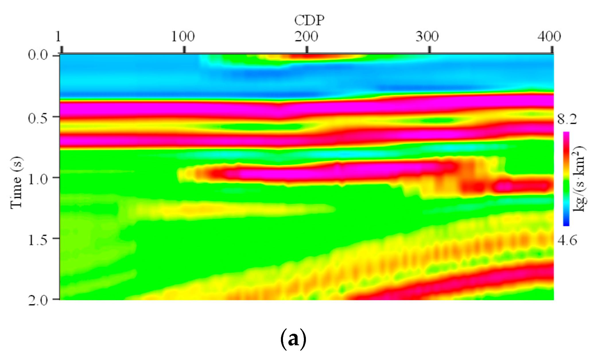The noise-tainted synthetic seismic data profiles are shown in Figure 1, where Figure 1a–c show the 15°, 25° and 35° profiles, respectively. The corresponding true EI model profiles for different angles are shown in Figure 2, where Figure 2a–c show the 15°, 25° and 35° profiles, respectively. From Figure 2, we can see that the true EI models contain thick layers, thin-bedded layers and some lenticular bodies.

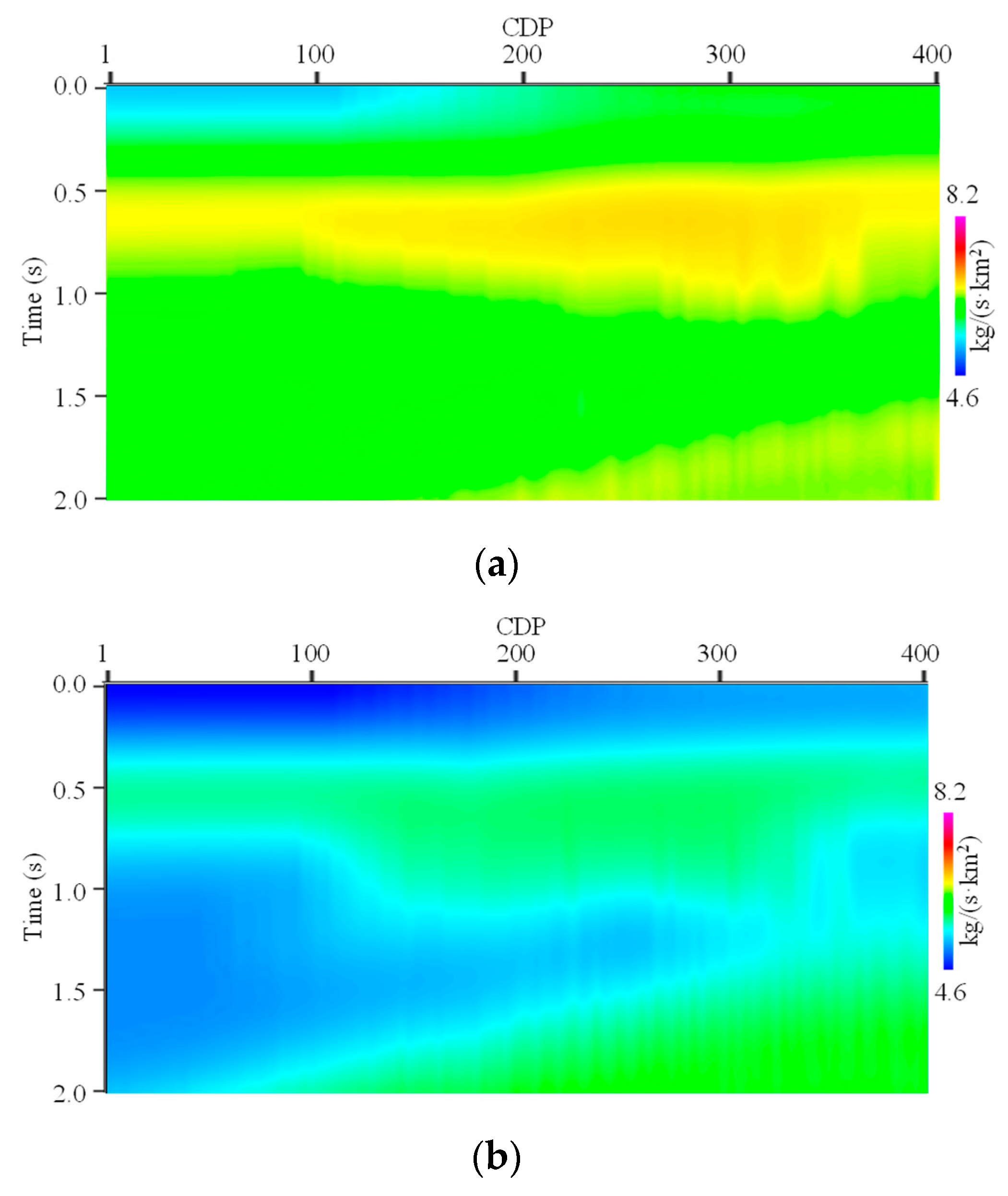
Next, a 15-Hz low-pass filter is carried out the true EI models. Figure 3 shows the low-frequency EI models for different angles, where Figure 3a–c show the 15°, 25° and 35° profiles, respectively. Then, the proposed EI simultaneous inversion (EISI) is carried out on the synthetic seismic data with the low-frequency EI models to serve as the a priori EI model. In this synthetic seismic data test, we set N_max = 100, λ = 0.1, μ = 0.1 and ε = 0.001. 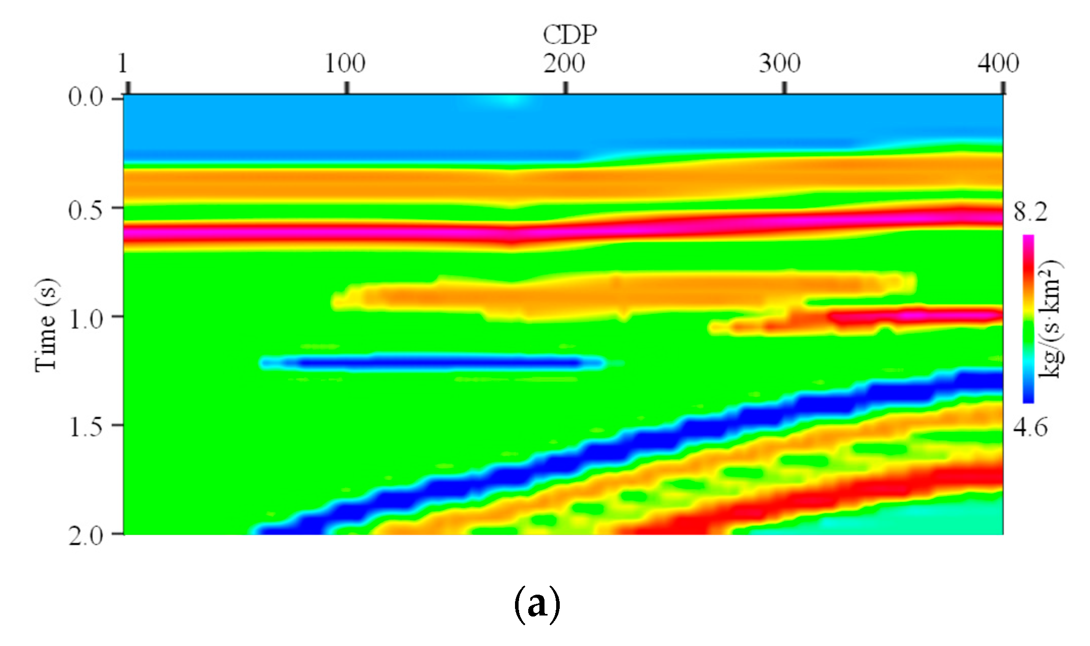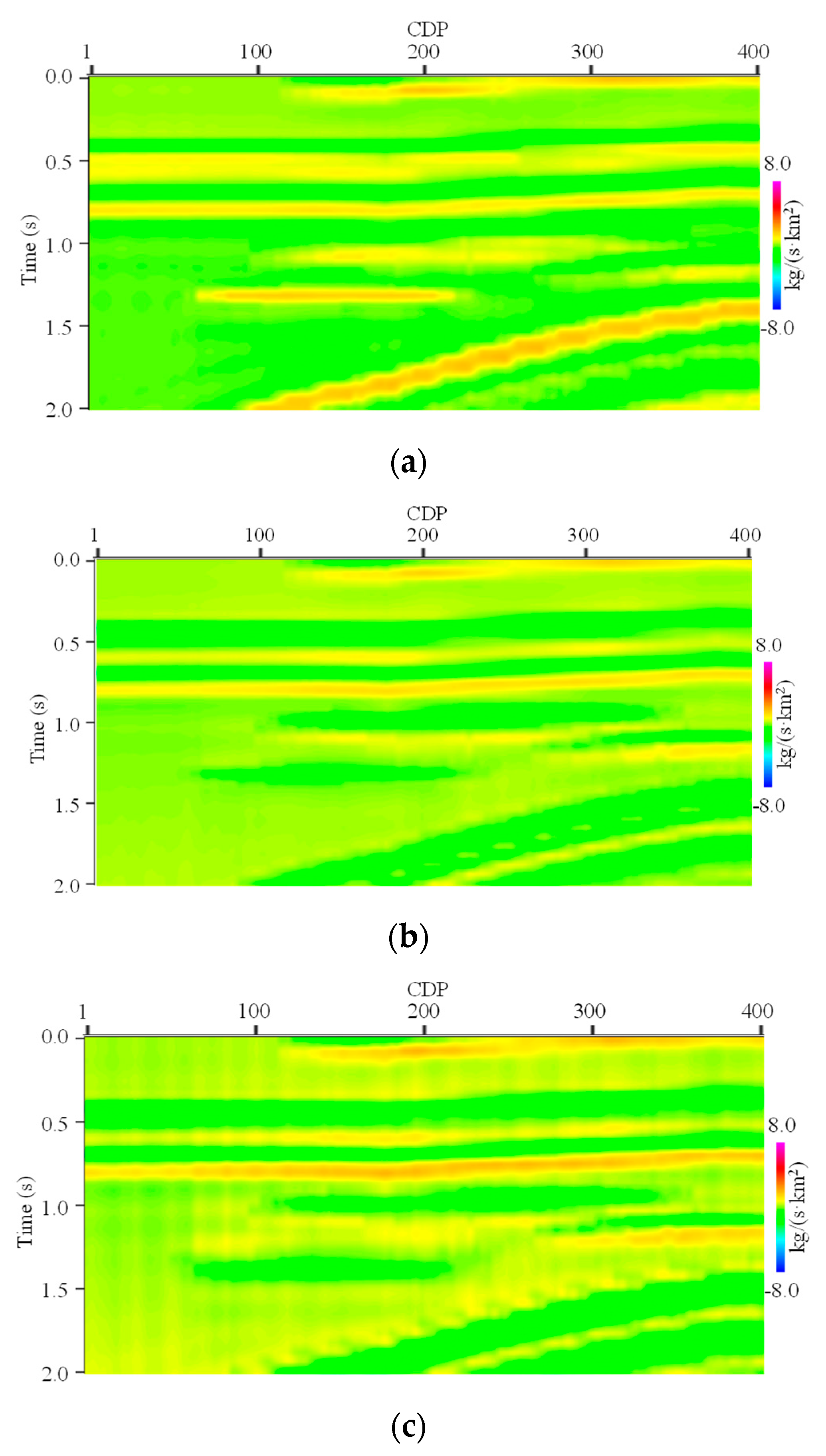Figure 4 shows the inverted EI models by EISI, where Figure 4a–c show the 15°, 25° and 35° profiles, respectively. From the comparison between Figure 2 and Figure 4, we can see that the inverted EI models by EISI faithfully match with the true EI models. The difference is small. The vertical boundaries of different strata in the inverted EI models are very clear. It is due to the sparse regularization constraint’s effect. In addition, there is conformity between different inverted EI models. The edges of the lenticular bodies in the inverted EI models are both very clear. The lateral distribution characteristics of both layers are also very clear.

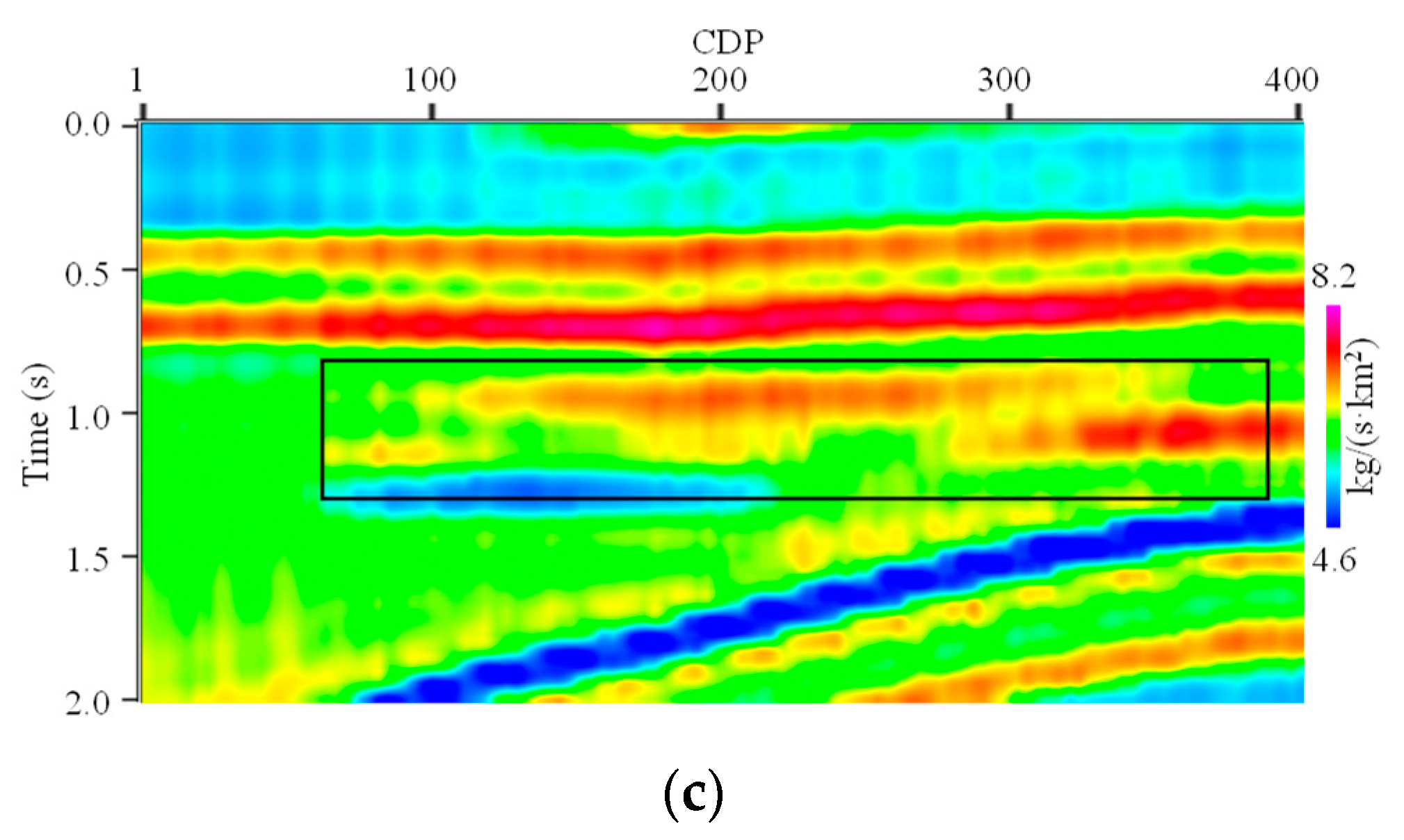
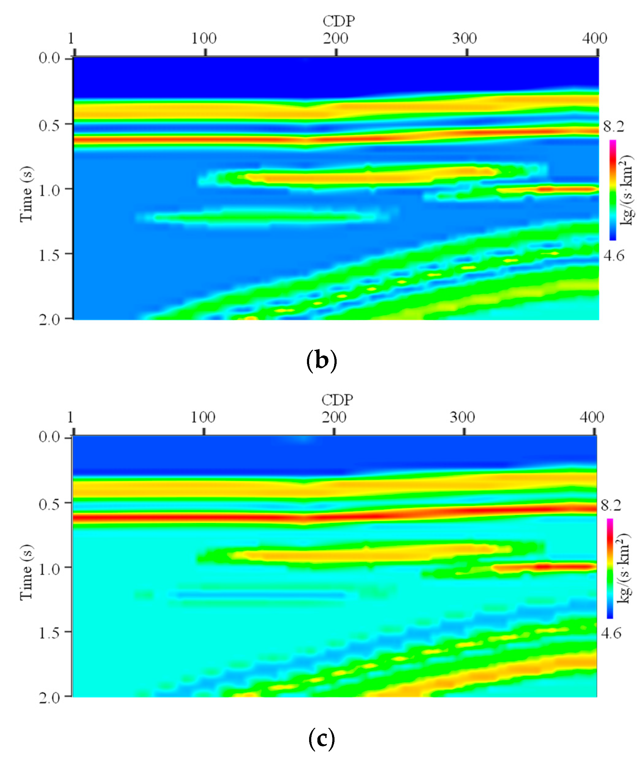
To show the superiority of EISI in conformity, conventional sparse regularization constraint EI separate inversion (CEI) is carried out on the synthetic seismic data with the same low-frequency EI models to serve as the a priori EI model. Figure 5 shows the inverted EI models by CEI, where Figure 5a–c show the 15°, 25° and 35° profiles, respectively. From the comparison between Figure 2 and Figure 5, we can see that the inverted EI models by CEI can also match with the true EI models. The vertical boundaries of different strata in the inverted EI models for small and medium angles are also clear. It is due to the sparse regularization constraint’s effect. However, the conformity between the inverted EI models for different angles is very poor. Especially in Figure 5c, the inverted EI model for a large angle, the vertical resolution, is relatively poor compared to the inverted EI model for a small angle, e.g., the inverted EI located in the black rectangular boxes. The edges of the lenticular bodies and the lateral distribution characteristics of the layers are very indistinct in Figure 5c.

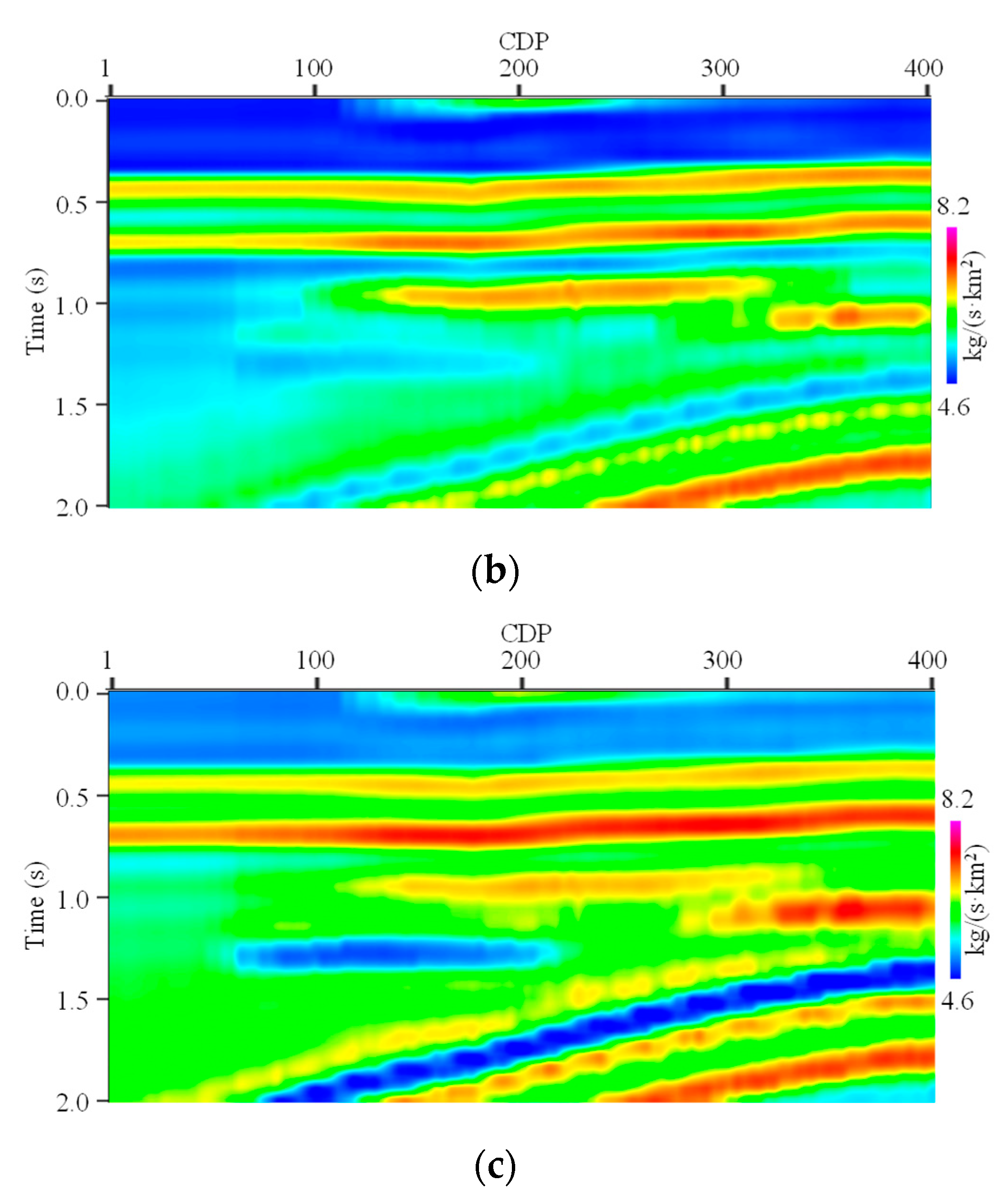
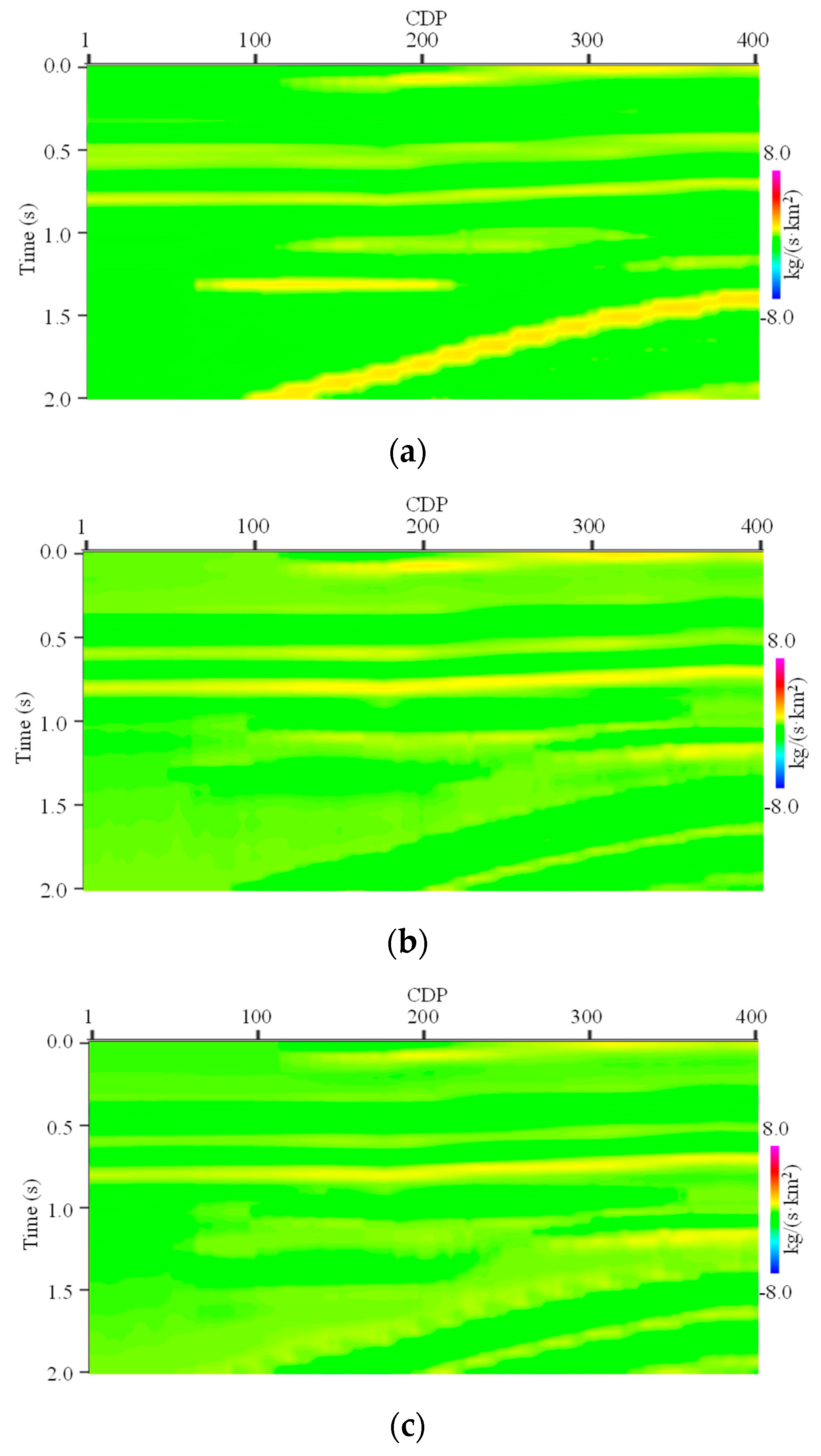
To further show the conformity in the EISI’s inversion results, Figure 6 shows the residue (i.e., misfit) between the inverted EI model by EISI and true EI model, where Figure 6a–c show the 15°, 25° and 35° profiles, respectively. As a contrast, Figure 7 shows the residue between the inverted EI model by CEI and true EI model, where Figure 7a–c show the 15°, 25° and 35° profiles, respectively. We can see that the magnitude of misfit in Figure 6 is significantly smaller than the magnitude of misfit in Figure 7.

To quantitatively compare the quality of the inverted EI models by EISI and CEI, we calculate the relative errors (RE) of the above different inverted EI models compared to the true EI models. The REs are listed in

Table 1. The REs of inverted EI models by different inversion methods.

Inversion Method	RE
EISI	0.0829
CEI	0.1576

. From Table 1, we can see that the REs of the inverted EI models by EISI are well below the REs of the inverted EI models by CEI.

From the test results of the synthetic seismic data, we can see that, compared to the CEI, EISI can not only clearly estimate the vertical boundaries of the different strata but also improve the conformity between the inverted EI models for different angles.

4. Real Seismic Data Applications

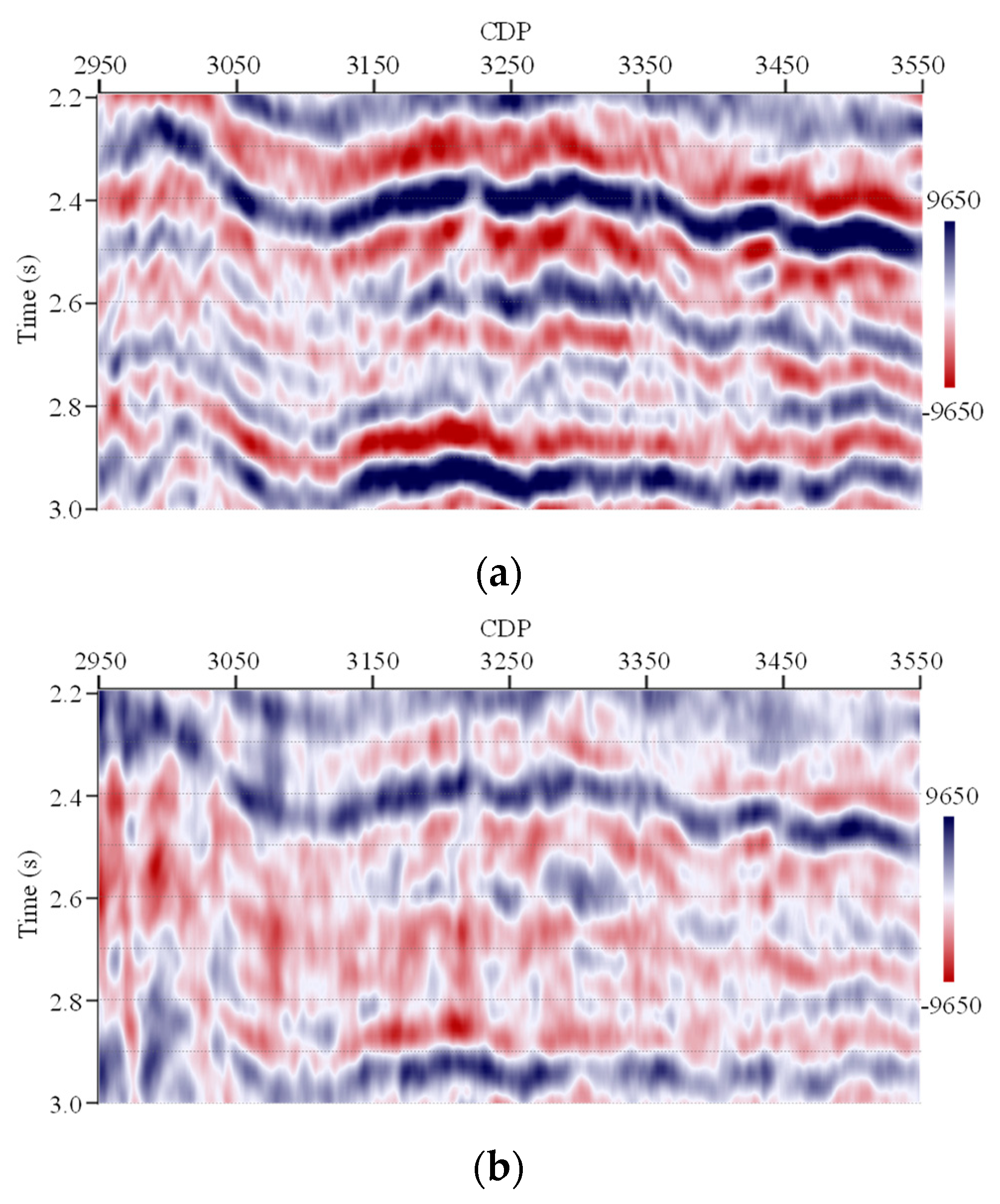
Next, a real seismic data line in Western China is used to test the feasibility of the proposed EISI in practice. This line contains two real partial angle stack seismic data profiles. The partial angle stack ranges are 11−20° and 21−30°, respectively. Figure 8 shows these two real seismic data profiles, where Figure 8a,b show the 11−20° and 21−30° profiles, respectively. These sections show similar tectonic structures but subtle amplitude variations. One can note the low signal-to-noise ratio of the large angle stack seismic data profiles.

Then, Kriging interpolation is used to build two EI models for two different angles with calculated EI well logs from the actual P-wave velocity, S-wave velocity and density well logs based on Formula (1). In the process of Kriging interpolation, the vertical variogram model is estimated from well logs, and the horizontal variogram model is estimated from seismic data. The angles for the calculating EI curves are 15° and 25°, respectively. After that, a 15-Hz low-pass filter is carried out on the interpolation EI models. Next, EISI is carried out on the two real seismic data profiles with the low-frequency models to serve as the a priori EI models. The angles used in the process of inversion are 15° and 25°, i.e., the median of the partial angle stack ranges. In this real seismic data application, we set N_max = 200, λ = 0.15, μ = 0.1 and ε = 0.01. 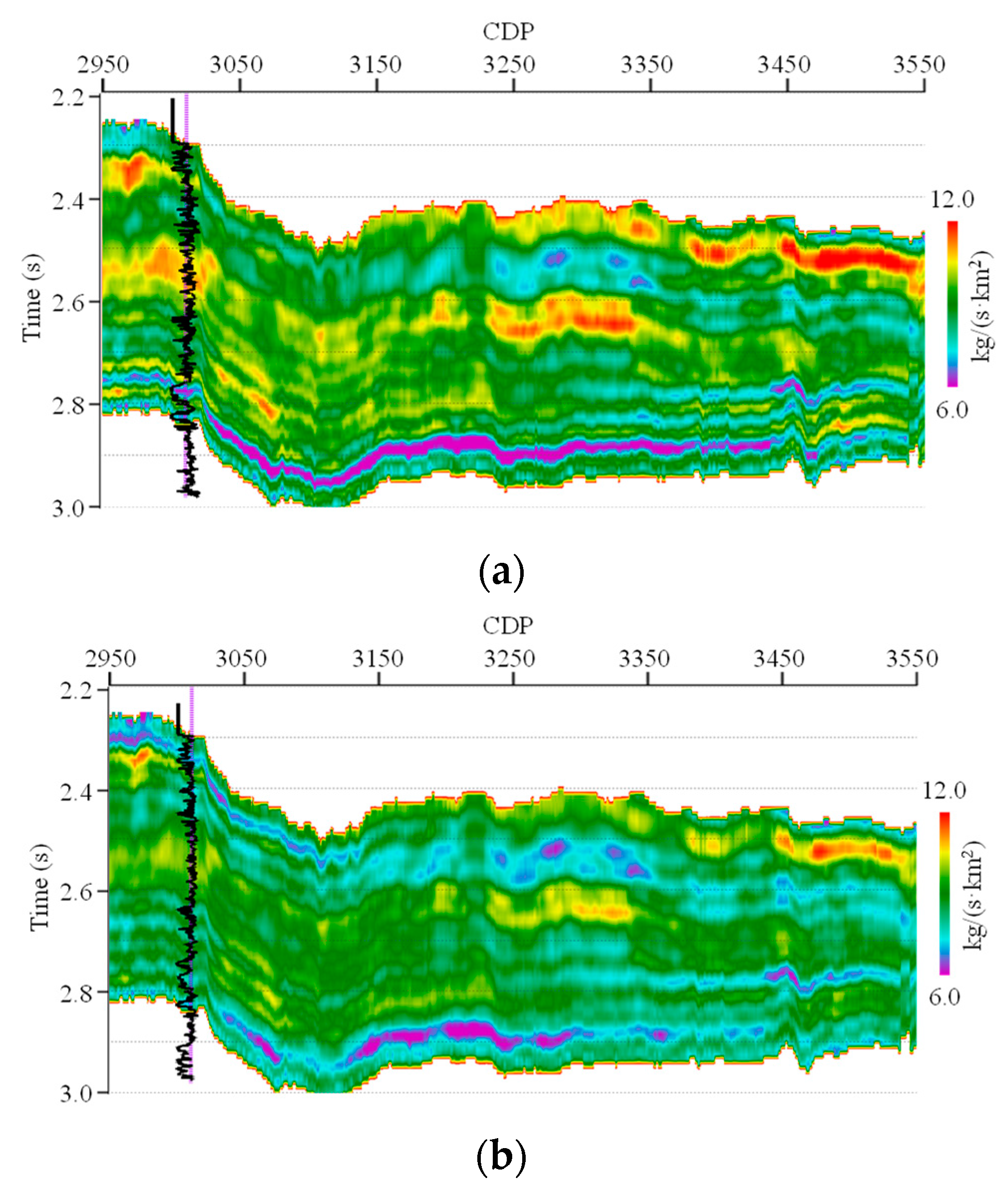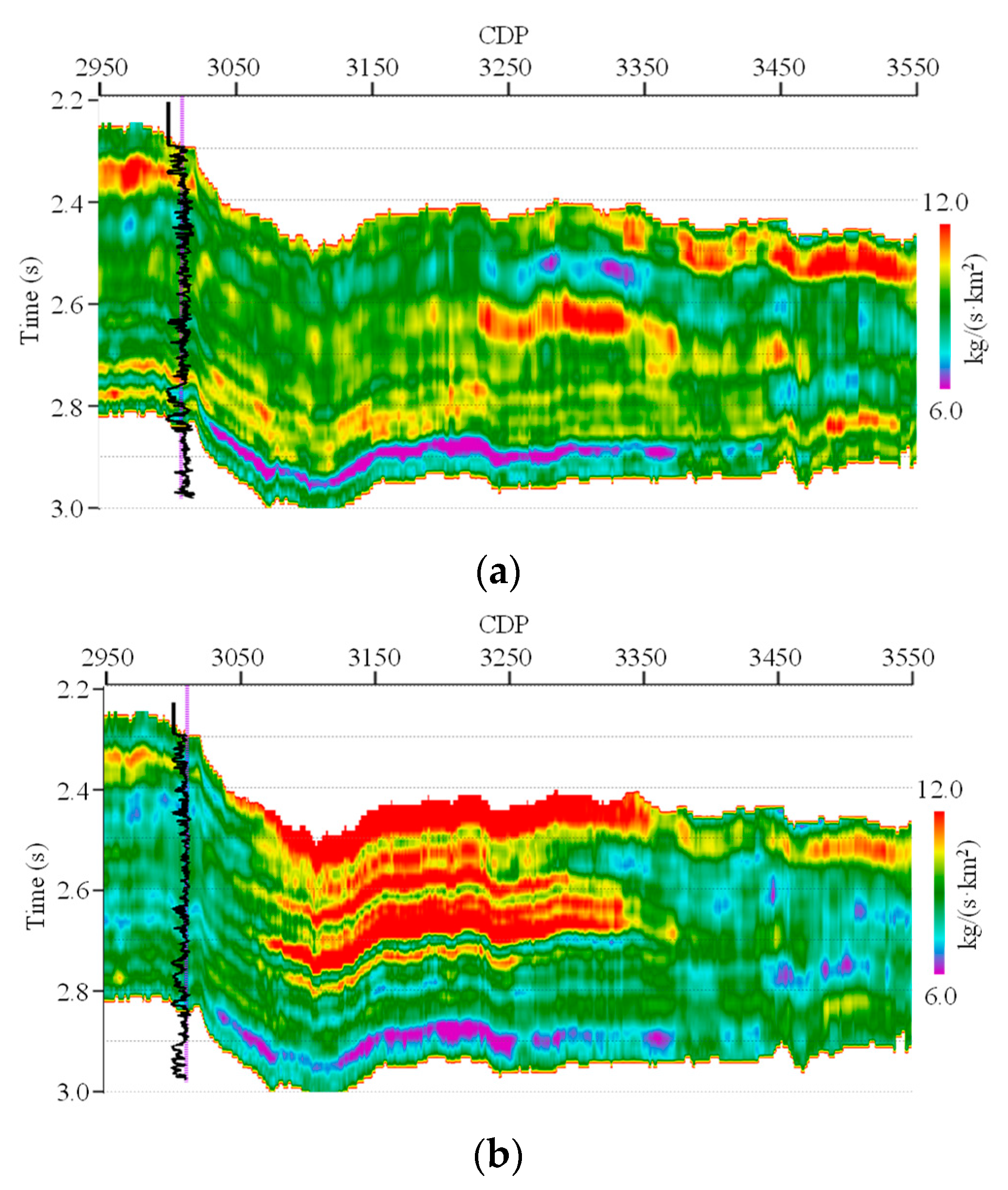Figure 9 shows the inverted EI profiles by EISI, where Figure 9a,b show the 15° and 25° profiles, respectively. We can see that the vertical boundaries of different strata in the inverted EI profiles are both clear, i.e., high vertical resolution. In the lateral direction, both the transverse distribution characteristics of the underground formations and the transverse interfaces of different faults are very clear. Hence, the inverted EI profiles for different angles by EISI also have good conformity.

Then, CEI is also carried out on the real seismic data profiles. Figure 10 shows the inverted EI profiles by CEI, where Figure 10a,b show the 15° and 25° profiles, respectively. We can see that the vertical boundaries of different strata in the inverted EI profiles for small angles by CEI are also clear. The vertical resolution in the inverted EI profile for a large angle by CEI is obviously below the inverted EI profiles for small angles. The conformity between the inverted EI profiles for different angles is poor. In addition, compared to the inverted EI profiles by EISI, the lateral distribution characteristics and the interfaces of the different faults in the inverted EI profiles by CEI are considerably less clear. Hence, the artifact produced by CEI is severe.

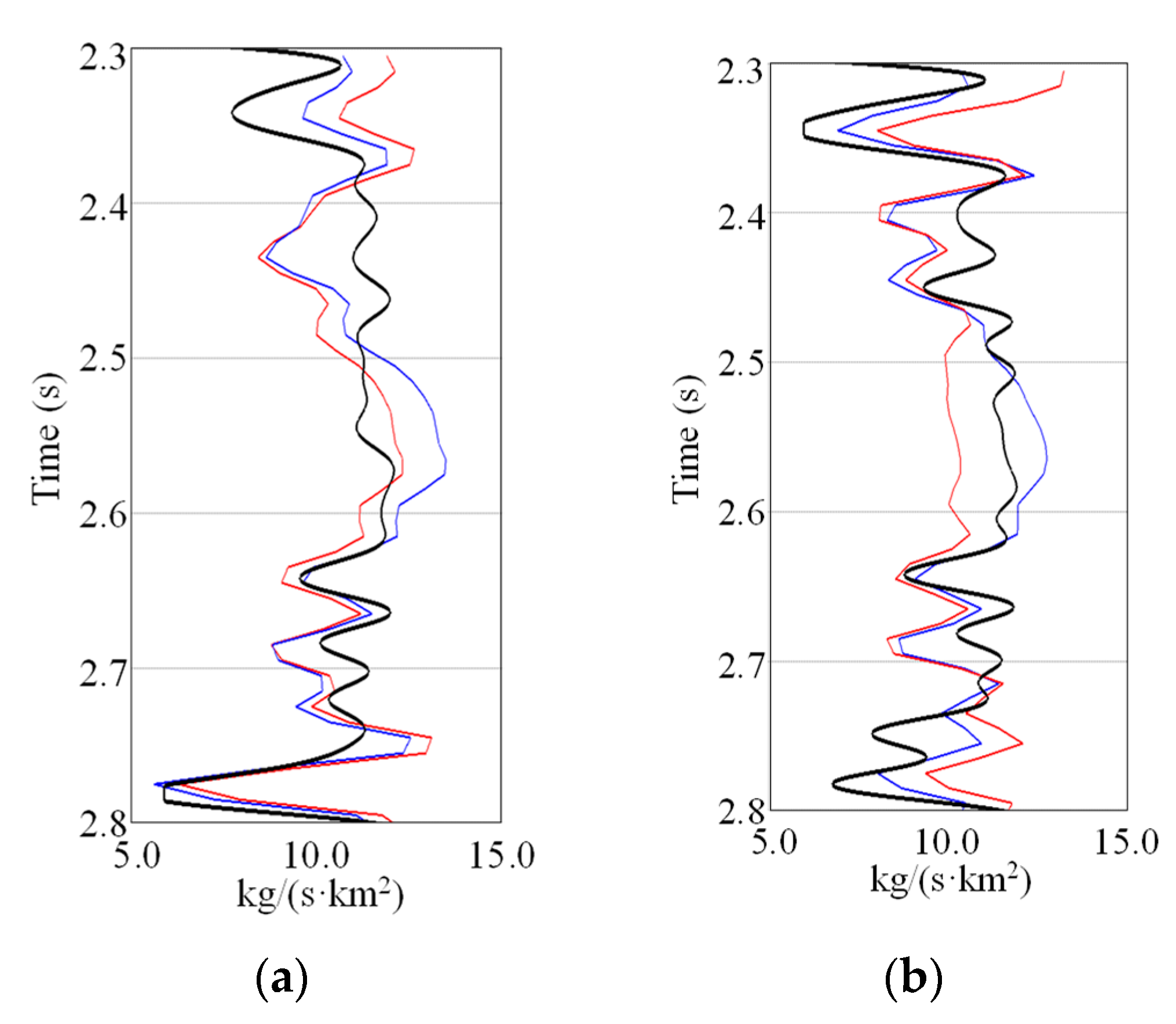
Figure 11 shows the single trace comparison between the well log curves and the inverted EI of the near-well seismic trace to see the values of EI, where Figure 11a,b show the EI curves of 15° and 25°, respectively. In Figure 11, the blue curves are the inverted EI by EISI, the red curves are that of CEI and the black curves are the well log EI. From the comparison, we can see that the values of the inverted EI by both methods can match with the well log EI. That is, the qualities of the inverted EI by the two methods are similar in the vertical direction. However, the conformity between the inverted EI by EISI for different angles is significantly better.

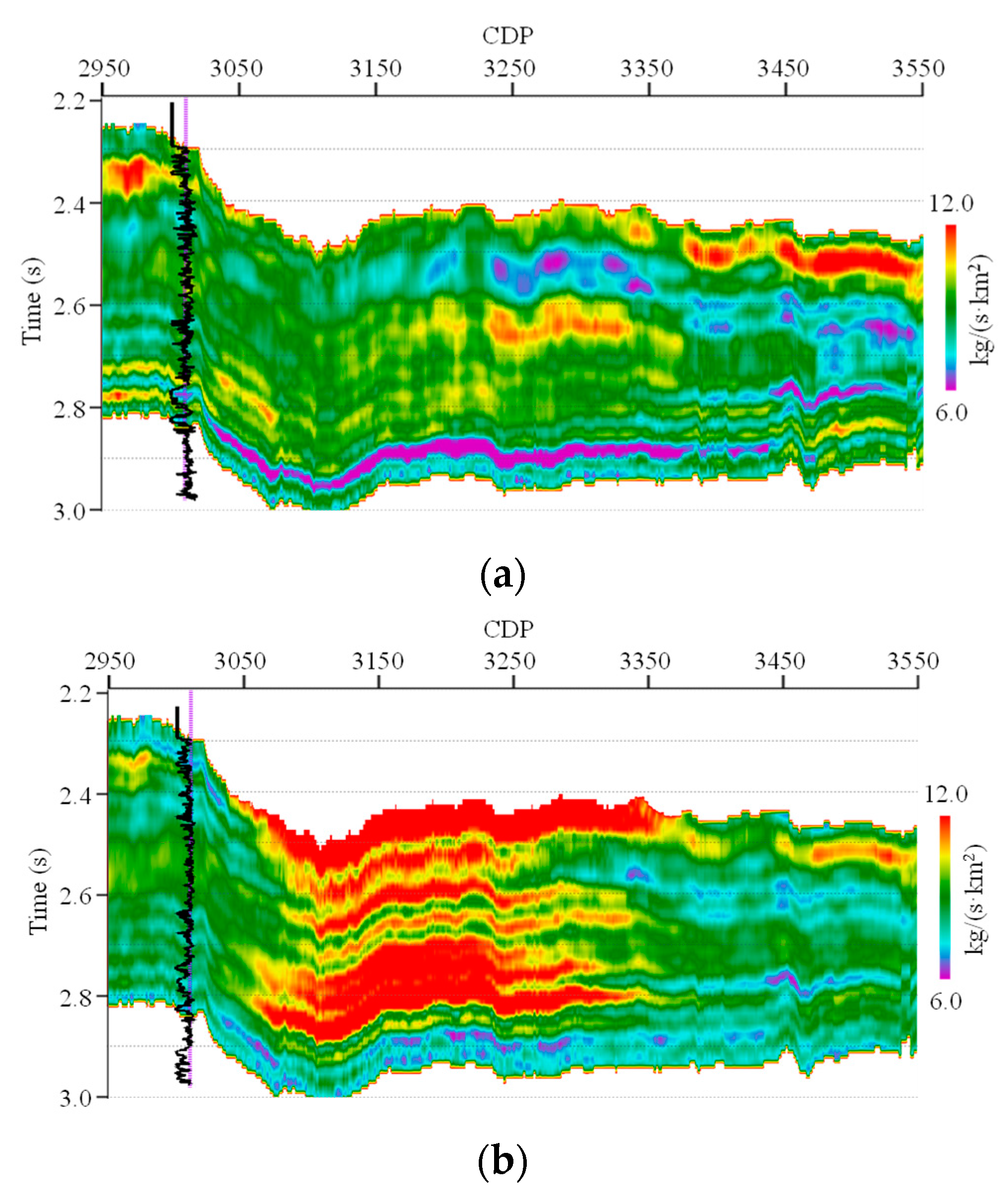
Furthermore, Figure 12 shows the inverted EI profiles by EEI, another existing conventional EI separate inversion method. We can see that the conformity between the inverted EI profiles for different angles is also poor.

From the real seismic data tests, we can also see that, compared to the conventional EI separate inversion, EISI can not only clearly estimate the vertical boundaries of the underground formations but also improve the conformity between the inverted EI models for different angles.

5. Discussions

In the theory of sparse signal representation and compressed sensing recovery, the joint sparse representation is proposed based on the similarity of multiple signals. It aims to reconstruct multiple unknown signals from a small number of observations that share a common observation operator and the same or similar support sets. In other words, when multiple signals have a joint sparse structure, their non-zero elements occupy the same or similar positions. If the multiple singles can be sparsely represented in some basis or dictionaries or through some sparse transforms, their sparse representation coefficients also share the same or similar support sets. If the multiple sparse signals are arranged in a matrix in columns, the matrix will become row-sparse [23,24].

In the existing references, L2,1-norm has been used to measure this row sparsity or joint sparsity [23,24]. For a matrix X, its L2,1-norm is defined as the sum of the L2-norm of the rows [23], i.e.,

$${\Vert X\Vert }_{2,1}={\displaystyle \sum _i{x}_i^T{x}_i}$$

(20)

where x_i is the ith row of X.

From the above exposition, we can see that, if one uses L2,1-norm as the joint sparse constraint in the EI simultaneous inversion, structure conformity of the inverted EI for different angles will exist. That is, the inverted EI for different angles has been imposed on a joint sparse structure, i.e., the non-zero elements in the corresponding reflection coefficients occupy similar positions. This ensures the structural conformity of the inverted EI at different angles. In this paper, we used Equation (8) as the joint sparse constraint. It contains the covariance matrix between reflection coefficients with different angles to consider the statistical correlation between them. It further improves the conformity between the inverted EI for different angles from a statistical point of view, and a statistical correlation certainly exists. The EI for different angles originate from the same underground geological medium and are defined by a set of the same parameters, i.e., P-wave velocity, S-wave velocity and density, except the incident angle.

Hence, there are some key factors that affect the quality of EISI in the process of inversion. First, the covariance matrix between the reflection coefficients with different angles must be effectively estimated. In this paper, we adopt the statistical calculation method, i.e., estimate the statistics from a nearby well control [29]. This is done by transforming the appropriate logs from depth to time and the generating the reflection coefficients with different angles. The covariance matrix is calculated over a time interval similar to the window, which is to be inverted. Second, the two regularization parameters λ and μ also greatly affect the inverted EI models. Here, the quality control method has been adopted to select these two regularization parameters [25]. That is, adjust the parameters to be selected, get the inversion result for each value and choose the one whose inversion result has the best match with the actual well log.

In this paper, EISI is performed on the deterministic inversion framework. Hence, the uncertainty assessment of the inversion result is limited [30]. Within this framework, the uncertainty can only be assessed by linearization around the best-fit inverse solution with a posterior covariance of the model parameters in view of the Bayesian point [30,31]. However, it cannot work in this paper. If one correlates the first term and the other two terms in Equation (5) to the likelihood function of the seismic data and the a priori information of the model parameters, respectively, the posterior covariance cannot be explicitly expressed due to the joint sparse constraint.

The uncertainty can be effectively assessed on the stochastic inversion framework, e.g., Bayesian inversion [30,32], or iterative geostatistical inversion [33,34]. Stochastic inversion defines the inverse solution as a probability density function on the model parameter space [30] and can evaluate multiple uncertainties from different data sources, such as seismic data, well data or geological uncertainty in the a priori model [30,31,35]. The inverse solution is achieved by sampling the model parameter space by Monte Carlo or by using a geostatistical sequential simulation [30,31,32,33,34,35]. The stochastic inversion approaches usually combine with global optimization algorithms to optimize the objective function, such as genetic algorithms [34,36], simulating annealing algorithms [37]. However, when compared with the deterministic inversion methods, these stochastic inversion approaches are normally much more computationally expensive [30].

To effectively evaluate the uncertainty of the inversion results of EISI, one may be able to perform EISI on the stochastic inversion framework. For example, we can use Equation (5) as the objective function of the iterative geostatistical inversion.

In fact, the traditional objective function of the iterative geostatistical inversion is usually based exclusively on the correlation coefficients or misfit between real and synthetic seismic traces [34]. In recent years, Azevedo and Soares proposed a method to explicitly incorporate some regularization constraints used in deterministic inversion into geostatistical inversion, such as the a priori model constraint [34]. In this paper, in addition to the a priori model constraint, we also used a joint sparse constraint. Similar to the method proposed by Azevedo and Soares, one may be able to incorporate the joint sparse constraint into a geostatistical inversion. However, we think that it is outside the scope of this paper. This can be a future research topic.

6. Conclusions

In this paper, we proposed to simultaneously invert multiple partial angle stack seismic data to obtain multiple EI models for different angles. In order to couple these multiple EI models, a joint sparse constraint was used to serve as a regularization term. Based on the regularized least squares inverse theory, we constructed the objective function for EI simultaneous inversion.

On account of performing the inversion angle by angle separately, the conventional sparse regularization constraint EI inversion cannot hold the conformity between the inverted EI models for different angles, especially for the large angle stack seismic data with a low signal-to-noise ratio, whereas the joint sparse regularization not only constrained the sparsity in the vertical direction but also imposed conformity between the inverted EI models for different angles.

From the synthetic data tests and the real seismic data tests, we can conclude that, compared to the CEI, EISI can not only clearly estimate the vertical boundaries of underground formations but also improves the conformity between inverted EI models for different angles. The inversion results of the synthetic data and real data showed that it provides an effective new alternative method to estimate the EI from partial stack seismic data.