Design and Computational Analyses of Nature Inspired Unmanned Amphibious Vehicle for Deep Sea Mining

Abstract

This paper presents the design calculations, implementations, and multi-engineering based computational constructions of an unmanned amphibious vehicle (UAmV) which efficiently travels underwater to detect and collect deep-sea minerals for investigations, as well as creative usage purposes. The UAmV is expected to operate at a 300 m depth from the water surface. The UAmV is deployed above the water surface near to the approximate target location and swims underwater, checking the presence of various mining, then extracts them using a unique mechanism and stores them in an inimitable fuselage location. Since this proposed UAmV survives in deep-sea regions, the design construction of this UAmV is inspired by hydrodynamic efficient design-based fish, i.e., Rhinaancylostoma. Additionally, standard analytical approaches are followed and, subsequently, the inimitable components such as wing, stabilizers, propellers, and mining storage focused fuselage are calculated. The computational analyses such as hydrodynamic investigations and vibrational investigations were carried out with the help of ANSYS Workbench. The hydrodynamic pressures at various deployment regions were estimated and thereafter the vibrational outcomes of UAmVs were captured for various lightweight materials. The computed outcomes were imposed in the analytical approach and thereby the electrical energy generations by the UAmV’s components were calculated. Finally, the hydrodynamic efficient design and best material were picked, which provided a path to further works on the execution of the focused mission. Based on the low drag generating design profile and high electrical energy induction factors, the optimizations were executed on this work, and thus the needful, as well as suitable UAmV, was finalized for targeted real-time applications.

1. Introduction

Unmanned Amphibious Vehicles (UAmVs), also known as underwater drones, are any submersible vehicles that can operate underwater without the presence of a human operator. UAmVs are commonly used in oceanic research for purposes such as measuring current and temperature, mapping the ocean floor, detecting hydrothermal vents, and so on. To carry out the aforementioned applications, the UAmVs rely heavily on digital cameras, magnetic sensors, ultrasonic imagers, seafloor maps, and bathymetry measurements. Remotely Operated Underwater Vehicles (ROUVs) and Autonomous Underwater Vehicles (AUVs) are two types of UAmVs. A ROUV is an unmanned submersible vehicle that is controlled by a person on a surface vessel using a joystick in the same way that a video game is controlled. The ROUV is connected to the ship by a series of cables, or tethers, which send electrical signals back and forth between the operator and the vehicle. Most ROUVs have at least a still camera, a video camera, and lights, allowing them to transfer images and videos back to the ship. To collect samples, vehicles may be outfitted with additional equipment such as a manipulator or cutting arm, water samplers, and instruments that measure parameters such as water clarity and temperature.

An AUV is an unmanned submersible vehicle that operates autonomously because it does not require real-time input or control from a human operator or driver. Before embarking on any complicated missions, the AUVs are generally programmed with instructions and then deployed into the ocean. AUVs can drift, glide, or propel themselves through the water, depending on their design. Propelled AUVs can travel faster and are more manoeuvrable than non-propelled AUVs, but they have less battery life and are typically used on missions lasting several hours to days. Non-propelled AUVs (drifters or gliders) either drift without power or glide up and down in the water column by changing buoyancy, making them much less manoeuvrable. The AUVs do not require a large and complex support system, but they do carry their energy source and thus do not require external power. The lack of external control lowers the operational cost of employing a human operator: Unlike other unmanned vehicles such as ROUVs, AUVs work without control from an operator, which makes it faster, increasing its data-to-signal ratio makes surveys faster and more accurate. The geographical positions to be followed, navigation requirements for following these positions, measures to avoid obstacles, measures to take if any equipment fails, and payload device operation procedures are all predetermined. For these reasons, the AUV is the most appropriate type for detecting and collecting seabed-based mining available up to 300 m below the water’s surface. As a result, this proposed UAmV is classified as an AUV.

1.1. Literature Review

A literature survey is a collection of previously completed and relevant studies that aid the researcher in gaining a complete picture of the short-listed problems, as well as providing the best methodology for solving the problems. It also provides support for implementing the proposed methodology. The literature review for this project is focused on the following themes: UAmV design and components, computational fluid and vibrational analysis procedures, analytical approach for energy extraction, details of suitable materials for UAmV, and mission execution capability and supporting components.

Muhammad et al. [1] showed the dynamic stability of an underwater glider, wherein two different forms of wings such as rectangular and tapered on hydrodynamic characteristics were investigated. They also explained the motion, which was based on six degrees of freedom (DOF). A highly manoeuvrable glider requires dynamic stabilities in both horizontal and vertical directions. The stability was controlled by eternal fixed wings and a rudder. The paper also explained the performance of the glider, i.e., glide ratio, horizontal, vertical, and sink were related to its hydrodynamic characteristics. This also provided steady-state CFD analysis to determine the hydrodynamic characteristics and dynamic stability of a glider. It concluded that the glider with tapered wing forms had a positive relationship between the velocities of the glider at the same angle compared to the rectangular wing. The rectangular wing had better dynamic stability with a high lift force. This shows that the CFD simulation results are important for the dynamic stability of the glider. Additionally, we also confirmed which wing form is suitable for our model based on this paper [1].

Finger [2] investigated the design space for VTOL (Vertical Take-Off and Landing) UAmVs and evaluated the performance by direct comparison with conventional aircraft. The VTOL combines the helicopter’s ability to take-off and land almost anywhere, with the speed range and load-carrying capability of a fixed-wing aircraft. The paper also showed a different VTOL aircraft that uses single and double propulsive units. The scope of this paper was limited to fixed-wing aircraft that use a propeller to convert the propulsion system’s power into thrust power. The endurance performance, mass fraction model, aerodynamic modelling, propulsion system modelling, propeller efficiency, fuel consumption, maximum engine power, etc. for the models were estimated. In this paper, the effects of the VTOL requirement on aircraft performance were assessed and this work showed that, with today’s technology, VTOL UAmVs are certainly feasible. It is clear from the paper that the VTOL aircraft gives better efficiency compared with conventional aircraft. This present work helps design the UAmV and performance of the UAmV. From this paper [2], we have finalized the configurations and design parameters for our work.

Chung et al. [3] defines the design process by defining performance requirements, the wing loading and associated power, the wing area mass and power requirements, motor size, and stability design based on selected material and wing area. The flight duration depends on the energy carried by the UAmV. High-energy fuel density enables lower weight and better performance; therefore, a method was developed by sizing the electric propulsion subsystem. Thus, the performance requirement of an electric-powered UAmV is defined as stall speed, the maximum speed at depth and turning radius, and the absolute ceiling is used to determine the wing load and power load. The UAmV’s wing area and power required can be calculated from weight and loading. The paper also gives a brief description of the conceptual design. The stall speed is a limit to the maximum speed at a safe lift. The cruising speed is 1.15 times the maximum lift-to-drag ratio and the maximum speed is 1.2 times the cruising speed. Then, it also gives the ceiling types and the critical performance. The paper described the weight estimation such as battery weight according to range and endurance, specific payload, and endurance. In aerodynamic configuration and stability design, the wing configuration greatly influences the aircraft’s aerodynamic characteristics and efficiency. It is necessary to understand the wing and aerofoil parameters to ensure that the aircraft has good aerodynamic characteristics under mission requirements. To increase the flying wing UAmV’s lateral stability, its dihedral angle was designed suitably. The manufacturing parameters are also given in this paper. The maximum cruising speed and design for the given payload are designed and reported in this paper. From this paper, the authors can determine the stable hydrodynamic design, the payload which we carry, the absolute ceiling used to determine the depth of the surveillance and energy fuels, and also able to determine its motor size with maximum cruising speed.

The study by Wood [4] focuses on the reasons for using AUV, highlighting its ability to help scientists carry out complex studies, such as the effects of metals, pesticides, and nutrients on fish abundance, reproductive success, and ability to feed, or on contaminants such as chemicals and biological toxins and the effects of plastics offshore. The paper also mentioned that there are currently over 50 types of AUV’s for research and commercial purposes, including gliders, which are vehicles that glide down slowly to a given depth and then return to the surface with a buoyancy effect. Gliders are capable of travelling in a horizontal path and a typical propeller follows saw tooth, which can descend or ascend vertically. There are several types of gliders. Among them are Slocum gliders, optimized for operation in shallow waters in coastal areas, and spray gliders, which are hydrodynamic in shape and give 50% less drag, so their range is up to 4700 km. Deep gliders are made out of a composite pressure hull of thermoset resin and carbon fibre and operate for one year in 4600 km missions. Both sea and deep gliders have been used in the hydraulic system to control their buoyancy. The military has developed an advanced underwater winged glider based on the air force’s flying wing design. The above paper also presents the systems in hybrid AUV-powered gliders, such as active buoyancy and trim control, fluid intake and sample taking system, communication and navigation, etc, highlighting knowledge about gliders and their types. It also provides the use of controlling the buoyancy to steer underwater. With this in mind, we can define the type of model we to use in our ideas in addition to the system required for underwater purposes and the efficient propulsive system for our requirements.

Abdullah et al. [5] highlights the convenience of computational methods for solving fluid flow problems. They give a brief definition of the gliders, in which the AUV dive and return with buoyancy and the gliders are mainly used to collect oceanographic data. The Lattice Boltzmann methodology (LBM) is used for the numerical background in place of meshing because the Meshing process is time-consuming. The paper showed that the bell span-load wing (BSW) shape was applied to the existing glider to improve the efficiency of the glider without considering its yaw and roll motion and, hence, the tail was not removed from the glider. The CAD (Computer-Aided Design) of the BSW-shaped glider and the lattice structures around it has been represented. After several calculations, it was shown that the BSW design generated less drag force than the elliptical span-load wings (ESW) design. In this paper, a wing design form was implemented to the benchmark glider design and the computations were taken, in which it was concluded that the lift and drag forces reduce while the stall angle increases. From this, it was seen that BSW provides less drag and lift forces. The variations in the drag and lift forces with the various AOA showed that the BSW shape design increased the stall angle of the vehicle. As shown in this paper, the BSW wing gives minimum drag compared to the ESW design; hence, it is clear that the BSW design is used to obtain better efficiency compared to the ordinary wing design.

Zihao et al. [6] suggest underwater gliders with low lift-to-drag ratios to solve the targeted problem, developing the flying-wing design. To optimize the shape design using the computational fluid dynamics code, further calculations were undertaken. CFD simulation was performed to investigate the hydrodynamic force at various velocities and angles of attack. It was used to determine the wingspan of the AUV glider. In the flying wing configuration, which was configured to travel farther in horizontal per unit distance and ascend vertically with great gliding efficiency, they used NACA 6 series aerofoil, which provided maximum laminar flow. The reason for selecting laminar flow aerofoil was that the Reynolds’s number of gliders is laminar and the turbulent transition layer in which the winglets under reasonable design can improve glide efficiency. The performance prediction suggested that the flying wing underwater gliders were more suitable for AOA, which was 5 degrees and had a small glide slope angle. The paper concluded that, in the future, further designs of the HFWUG will be carried out. Appendages of the glider, such as a winglet—a flap that can reduce the drag and enhance manoeuvrability—will be developed. It is clear that the flying wing configure improves the performance and is more suitable for big AOA.

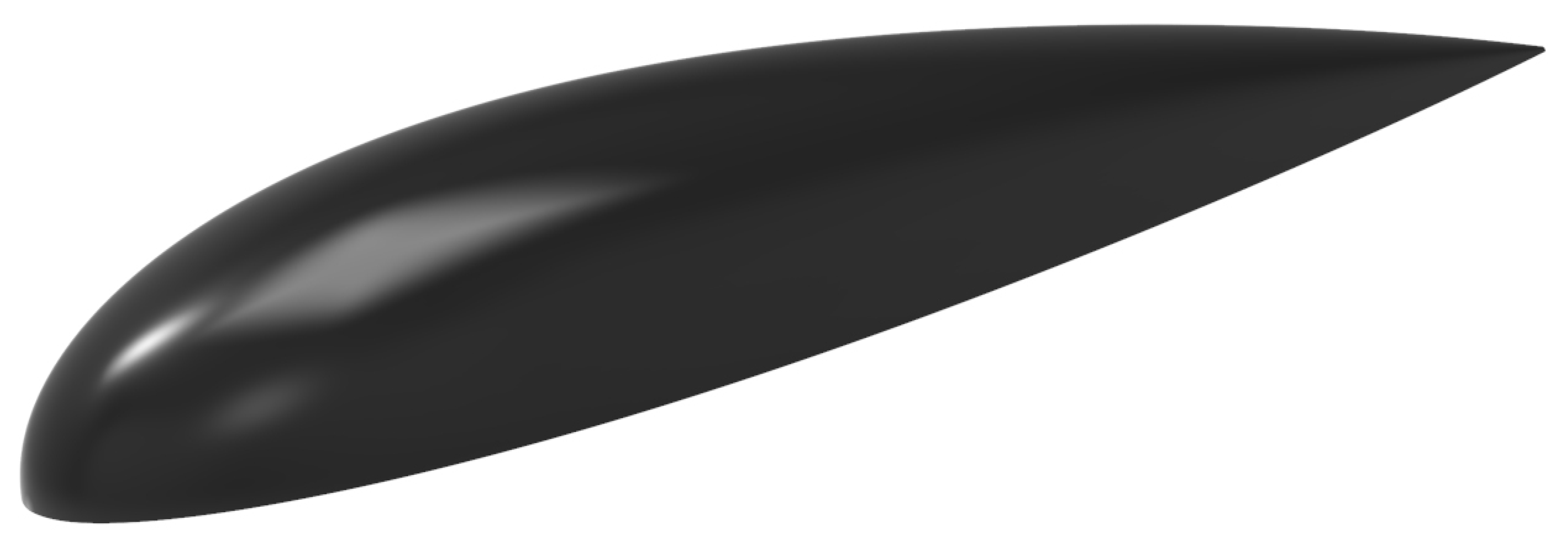
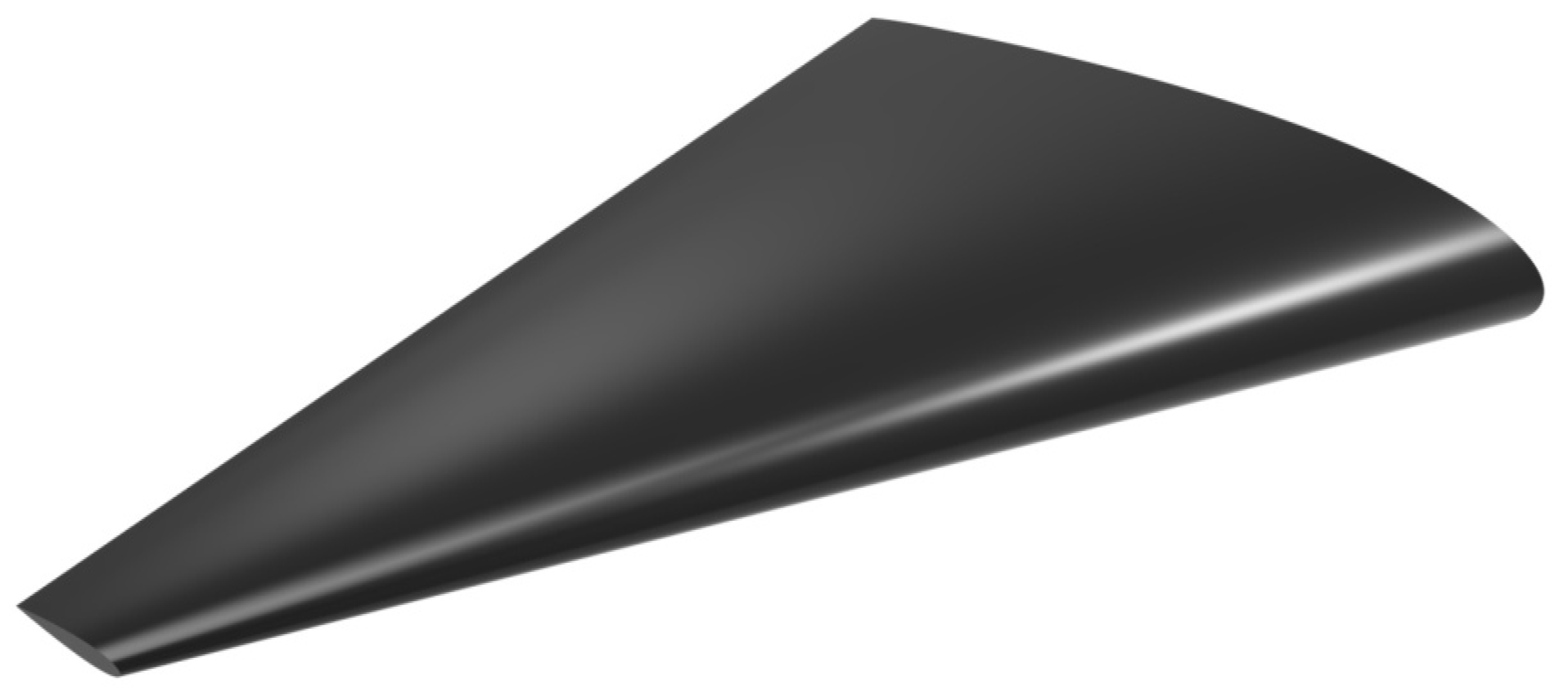
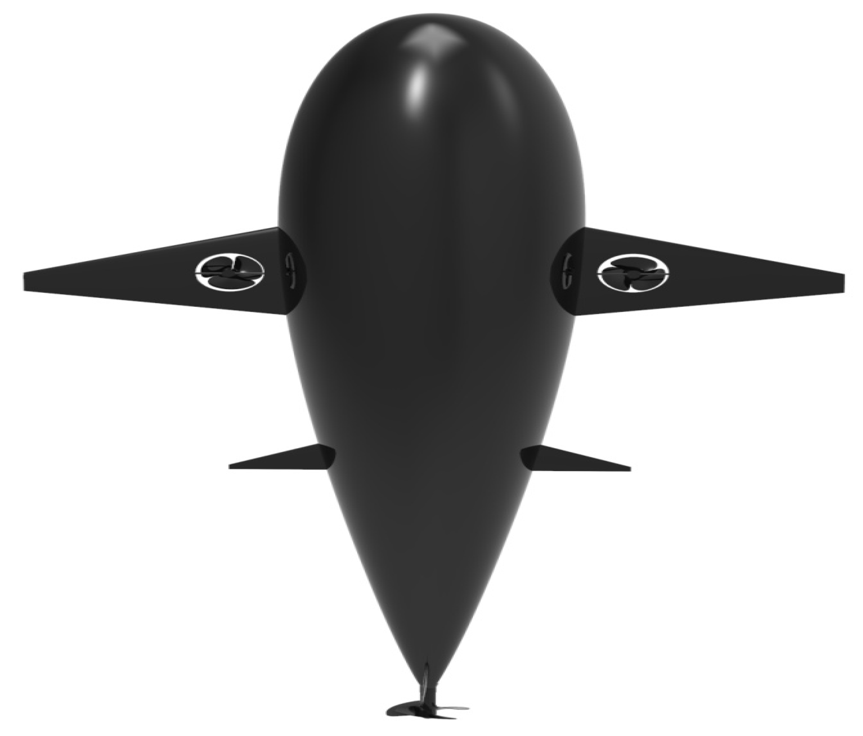
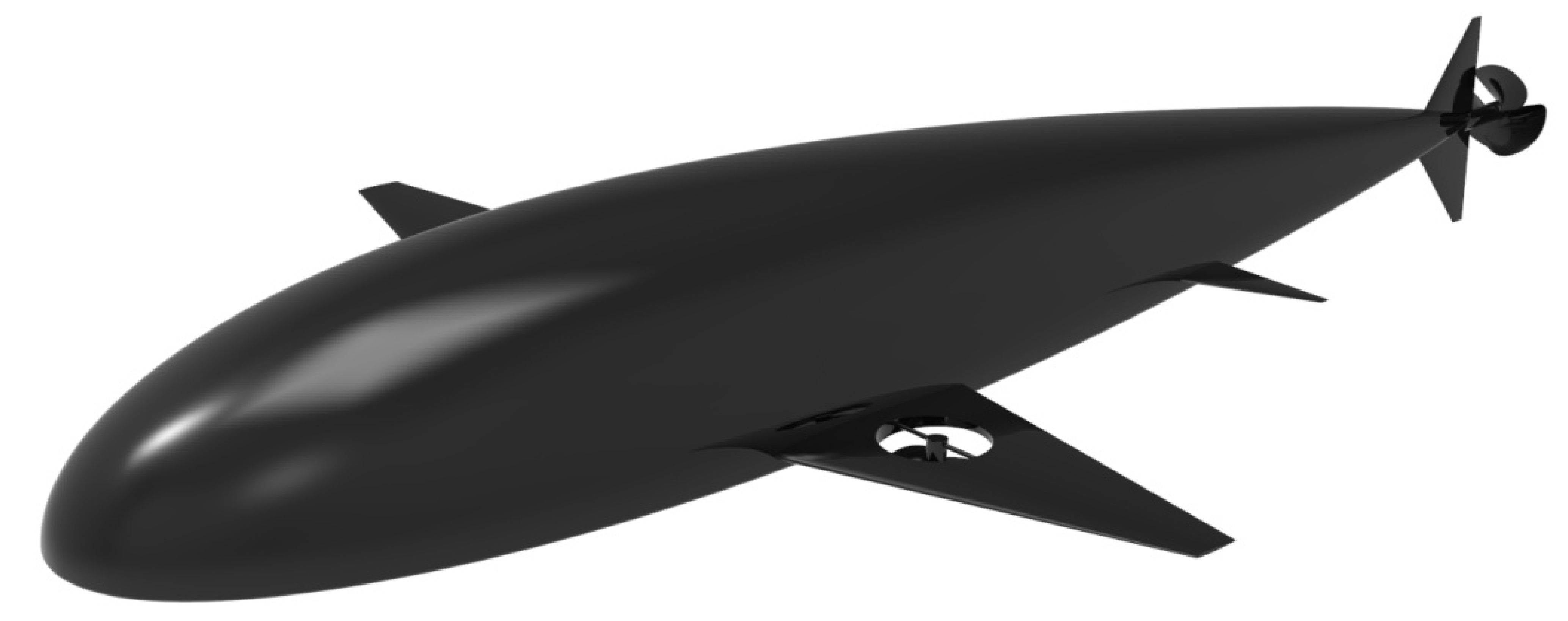
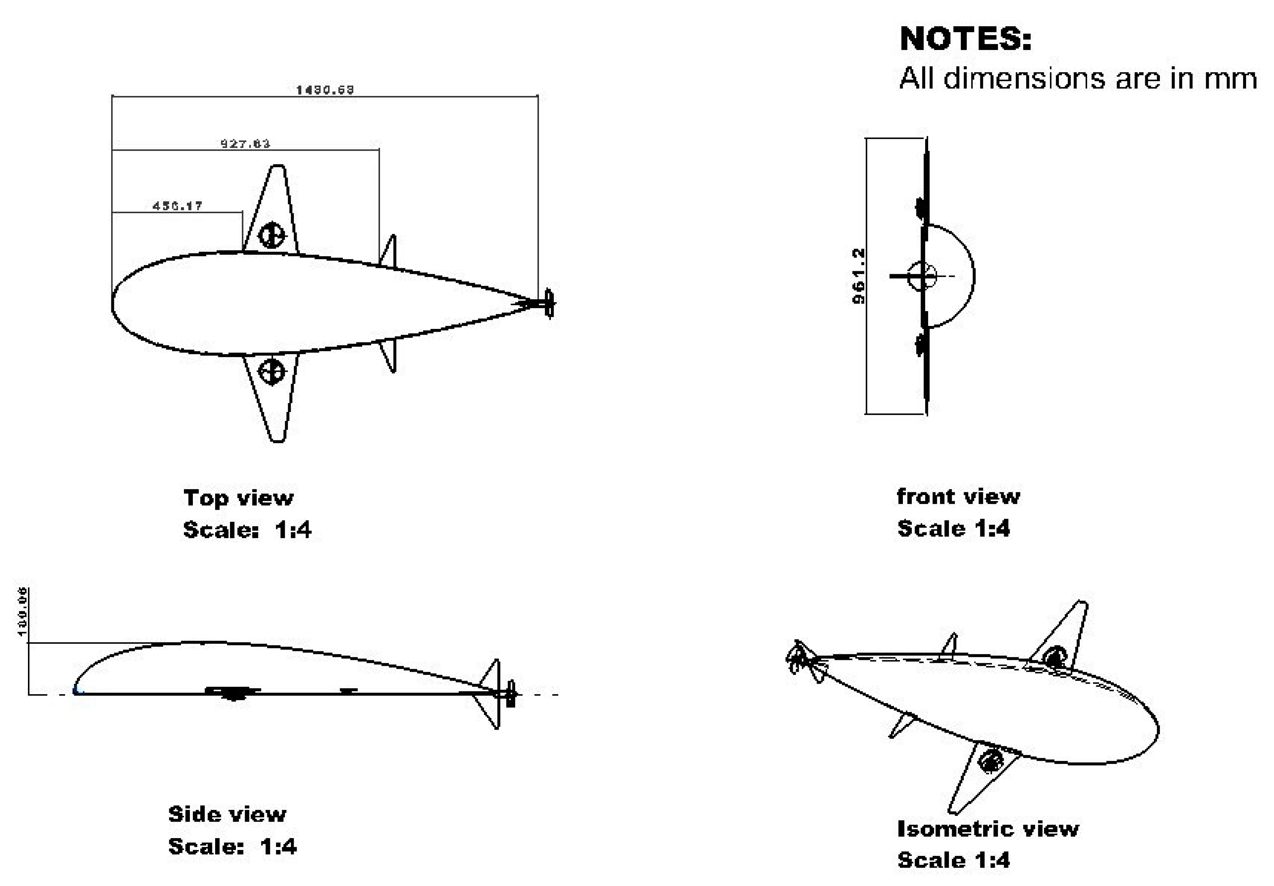
Since the targeted mission location is very dangerous, in order for the UAmV to withstand high hydrodynamic pressures, the need for an efficient, structurally robust, streamlined design is essential. Therefore, this work proposes a design that mimics the appearance and ability of deep-sea fish. 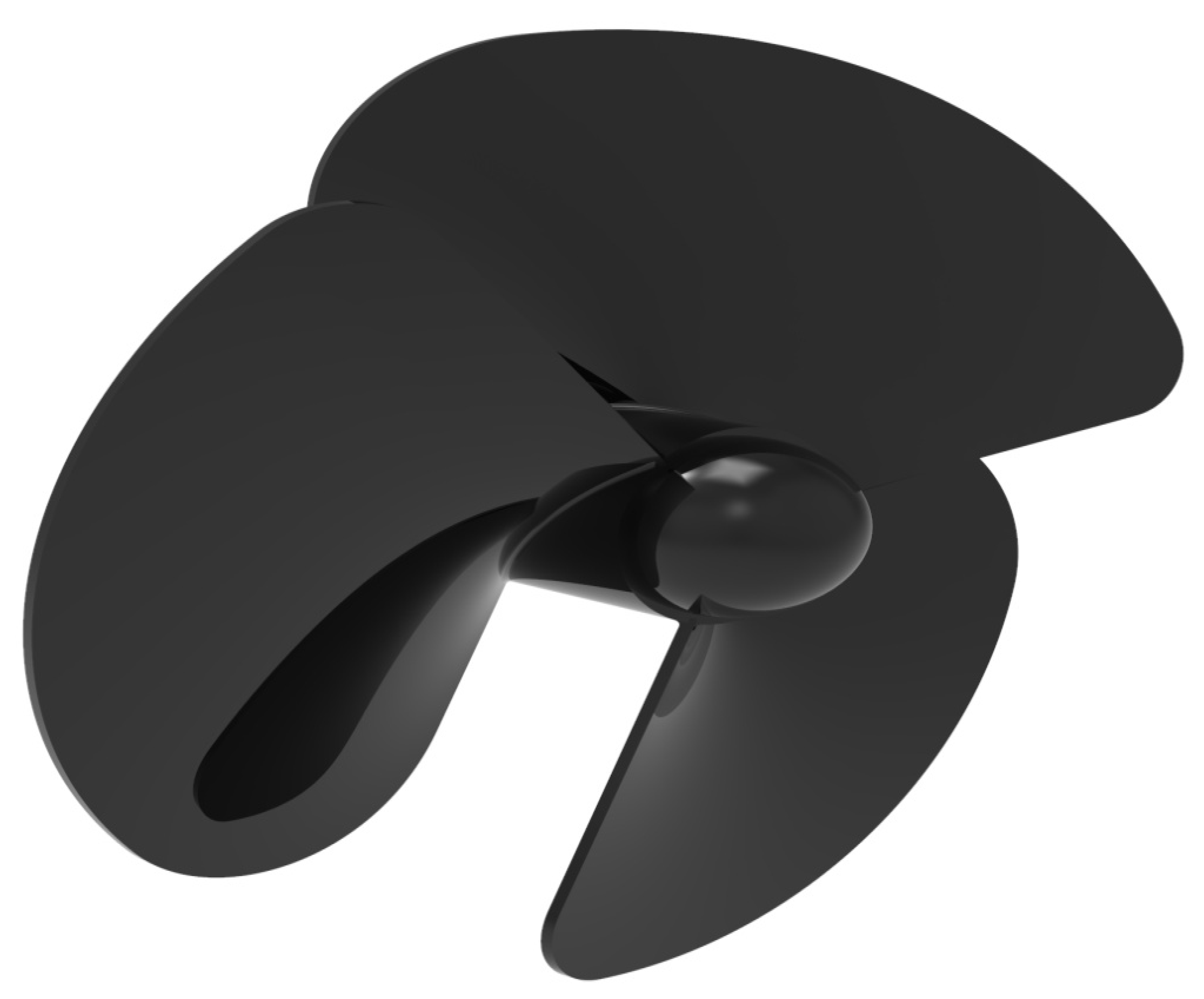According to the data based on the first literature survey, a design based on Rhinaancylostoma was found to be the most suitable to carry out the current investigation [7,8,9,10]. Since the extremities of the UAmV were inspired by Rhinaancylostoma, it was also suggested that the length and breadth of the UAmV also mimic this species. The UAmV was therefore similar in length to Rhinaancylostoma. Additionally, the finalized wing, already introduced in this work, was straight tapered, the finalized horizontal stabilizer shape was straight tapered, and the shortlisted vertical stabilizer design was backward tapered. According to the data based on the second literature survey, conventional analytical approaches were used to design the wings and stabilizers, while the fuselage, forward propeller and vertical propeller were designed following unique analytical approaches [11,12,13,14,15]. When analysing other studies on the development of unmanned marine vehicles and their components, the authors noticed a few problems. The first problem was that the same propulsive system failed to provide a perfect needful thrust for both the aerodynamic and hydrodynamic environments. The second was that in the previous studies, wings were used instead of fins, but these imposed wings produced an additional lift, causing the smooth flight of the UAmV to collapse. Thus, this work predominantly focused on implementing an optimized wing that could not collapse the smooth lift. This is why this proposed configuration is regarded as the best. Additionally, through CFD, the drag and lift forces at various locations were computed, providing the working conditions and handling capabilities of these components of the UAmV.

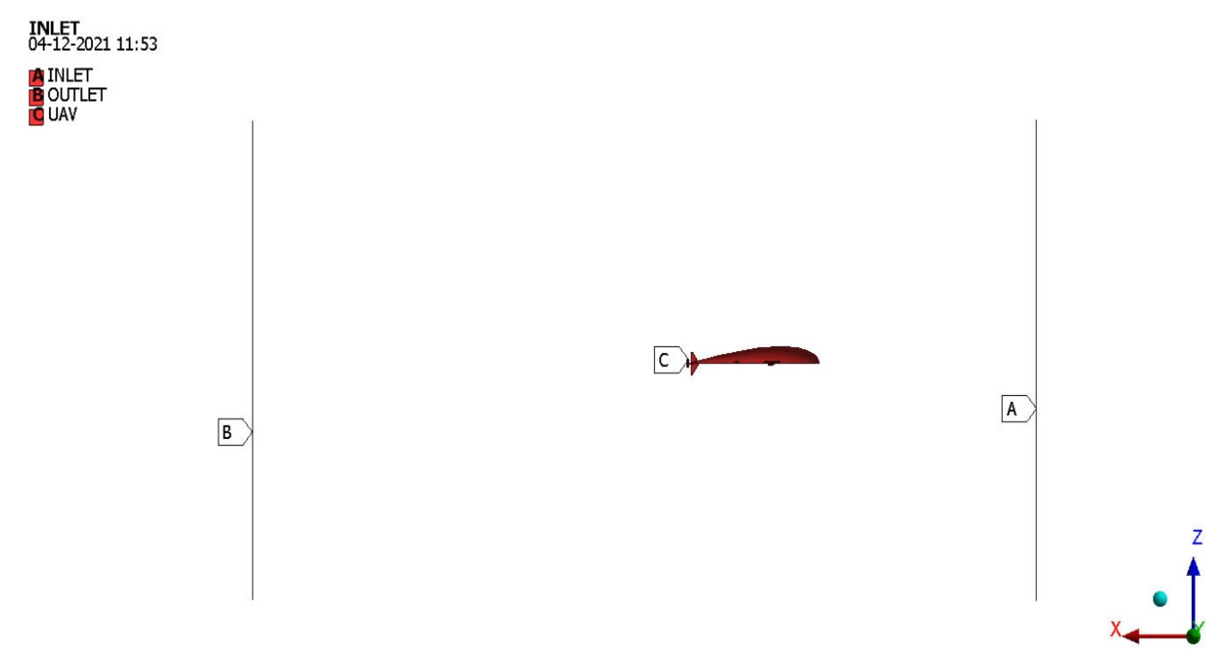
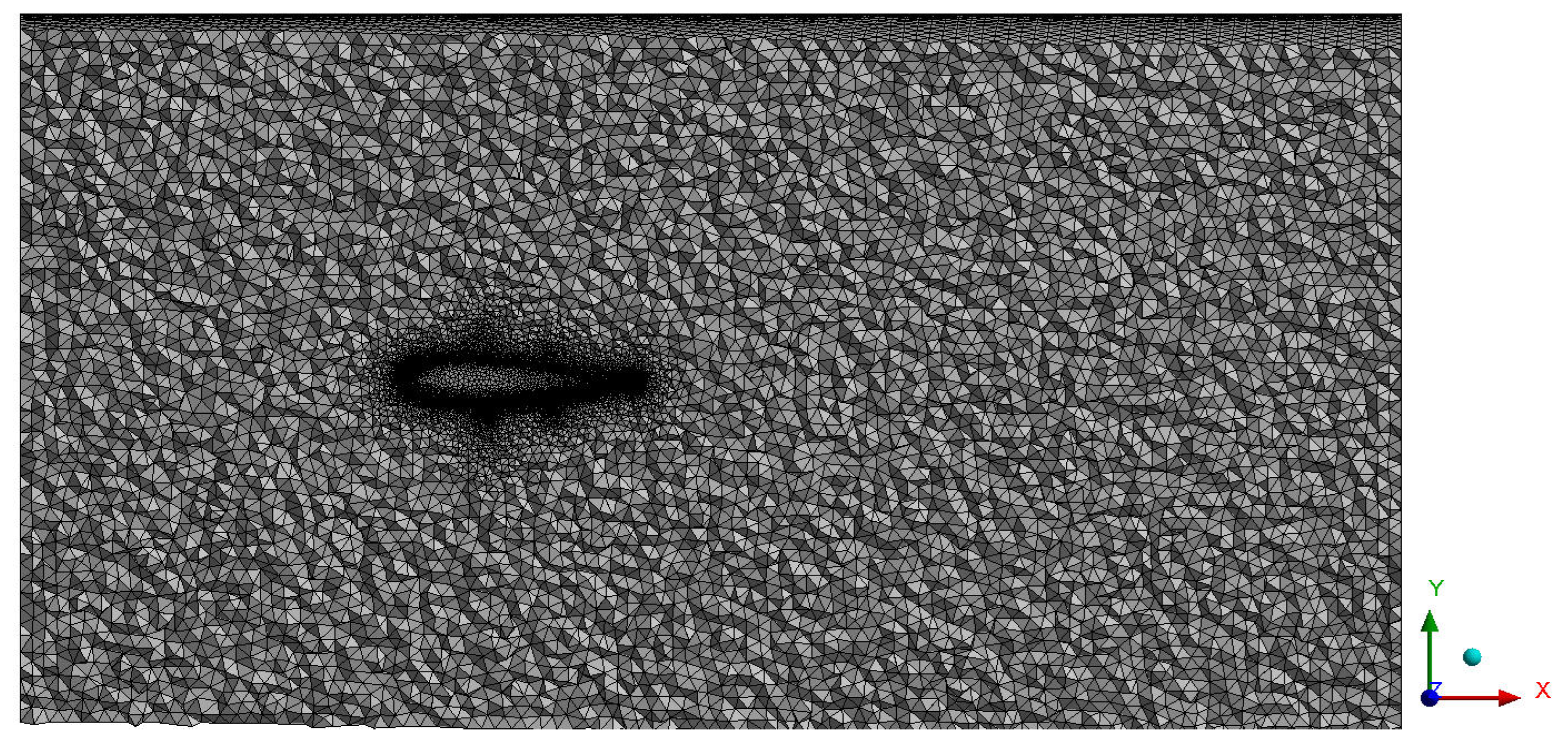
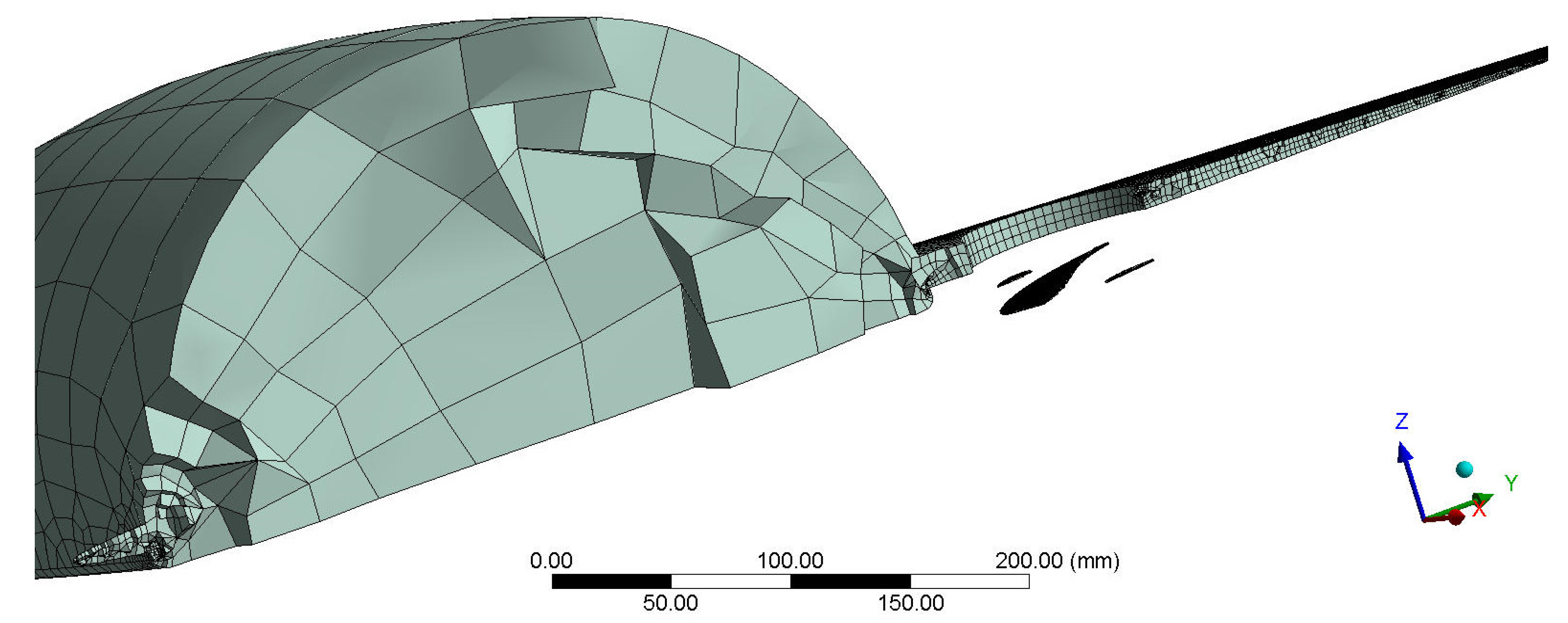
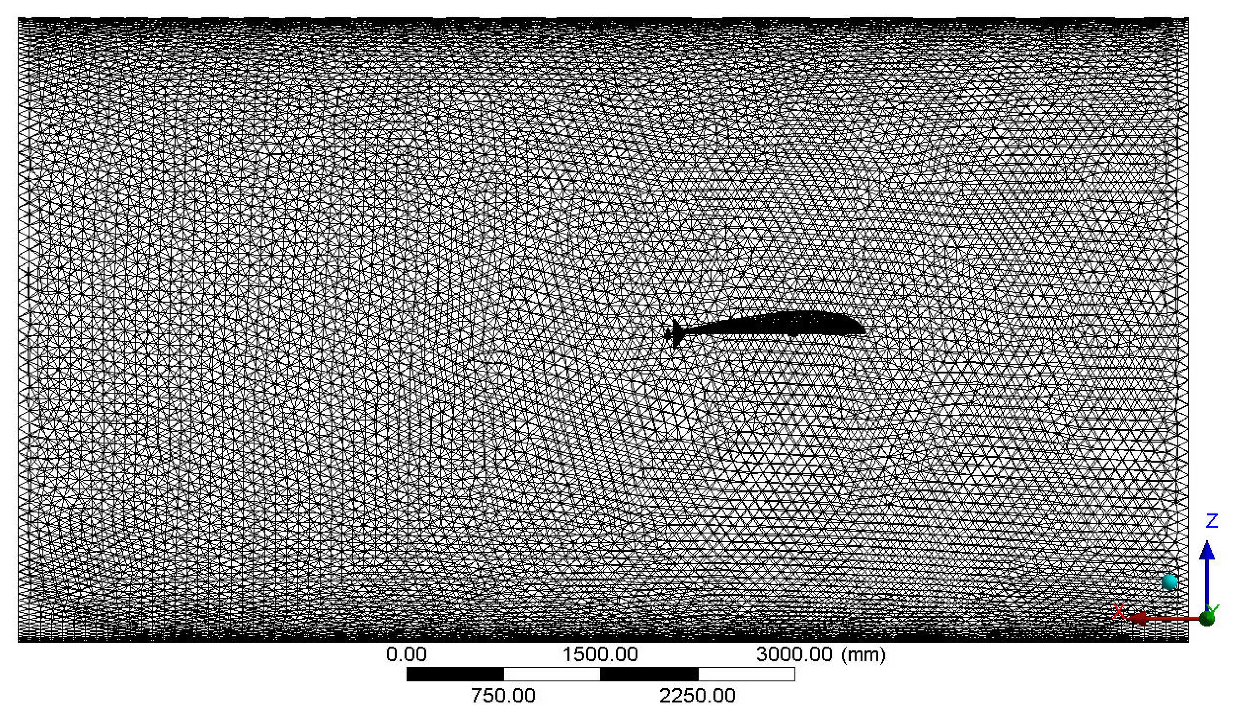
After a method was developed for constructing this UAmV, the next major phase comprised domain preparation, discretization, and computational procedure. These phases are based on data from the third literature survey [16,17,18,19,20,21,22]. Since the authors of this current work have predominantly relied on the ANSYS Workbench tool for all kinds of computations, this third sub-section is filtered and focused only on obtaining the boundary and initial conditions relevant for the aforesaid computational set-up. The information about the development of control volume, procedures to develop structural meshes, and procedures to attain reliable outcomes for computational hydrodynamic simulations were obtained [16,17,18,19,20,21,22]. Apart from the primary conditions, the secondary conditions provide significant support in computational fluid dynamic (CFD) simulations. The secondary conditions are a selection of suitable turbulence models and their additional enhancements, such as viscous heating, buoyancy effect consideration, etc., the selection of a suitable coupling scheme between fluid properties, and the provision of perfect values for turbulence models, such as value for viscosity ratio, value for hydraulic diameter, value for eddy length-scale ratio, etc. The incompressible flow-based computations were considered based on data from the fourth literature survey, and so the abovementioned conditions were determined [23,24,25].

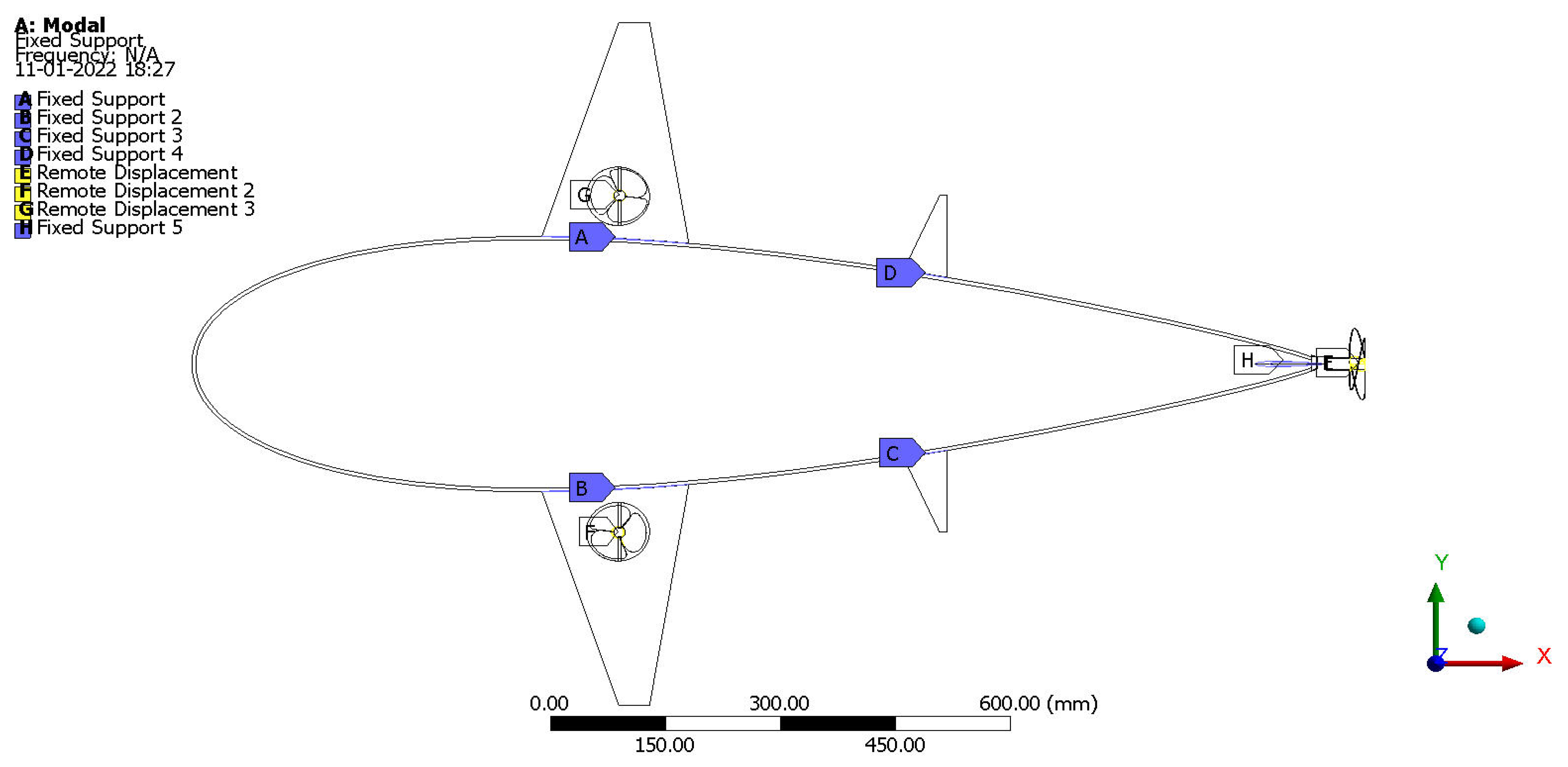
Aside from the CFD observations, computational vibrational analyses (CVA) also play a vital role in this investigation. The essential computational data for CVA were planned to extract from the fifth literature survey. Noted observations from this survey included an analytical approach carried out for the extraction of electrical energy through piezoelectric patches. The formula for this analytical approach included the important supports fixed on the object and the remote displacements implemented on the rotating components [26,27,28,29,30,31]. Additionally, the suitable material to withstand under fluid dynamic loads, as well as a suitable material to undergo high energy extraction-based observations, was executed. Density, young’s modulus, bulk modulus, and Poisson’s ratios, especially, were major focused initial conditions for computational structural analyses. Hence, the works [32,33,34,35] executed were supported hugely to attain the aforesaid properties. Finally, earlier applications completed by the UAmVs were collected, wherein the involvement of major and minor components for their mission executions were completely recorded. Through these studies [36,37,38,39,40,41,42], the selection of electrical and electronic components for this current work was executed.

Finally, aerodynamic and hydrodynamic forces generation and their components were studied, wherein the aerofoils imposed on the development of various components of UAmV were focused majorly. Primarily, the authors found that NACA profiles-based aerofoils were implemented on the various kinds of Unmanned Underwater Vehicles, which vary from slow to high-speed operational vehicles, low to heavy payload-based vehicles, short to long-range and endurance-based vehicles. Through focused study, more than twenty-five relevant aerofoils were found to be existing users in the UAmVs. The complete list of relevant aerofoils is listed in

Table 1. The detailed data of NACA-based aerofoils imposed in the development of UAmVs.

References	Aerofoils Used	References	Aerofoils Used
[14]	NACA 4412	[43]	NACA 0015, and NACA 0020
[20]	NACA 0015	[44]	NACA 0022
[21]	NACA 2408	[45]	NACA 2414
[22]	NACA 0015	[46]	NACA 0020 to NACA 0010
[47]	NACA 0012, NACA 0014, NACA 0016, NACA 0022, NACA 0008

. Additionally, symmetrical aerofoils were used predominantly in UAmVs rather than unsymmetrical aerofoils. The symmetrical aerofoils implemented in the components of UAmVs were fins, tail portions, and wings. Additionally, the selection of an aerofoils phase was completed with the support of Table 1.

From Table 1, it was found that symmetrical characteristics-based NACA aerofoils were used in all kinds of UAmVs. Based on the literature surveys, the authors developed four research articles [14,20,21,22] that demonstrate the major constraints on the development of symmetrical NACA aerofoils-based UAmVs, wherein the required lifts were achieved in all the cases for the maximum speed of 15 m/s at various angles of attack. Technically, the flow in and over this current UAmV is mostly laminar, so the implementation of low Reynolds Number-based aerofoils in this work has been suggested. Since hybrid configuration is proposed in this work (the separate VTOL propellers for depth increment and decrement, also hovering), the various angle of attack-based computations are avoided.

1.2. Proposed Concept for the Collection of Deep-Sea Minerals

Due to the fact that this UAmV is able to thrive in more difficult circumstances, traditional construction is unsuitable for this design and development. Thus, both visibly and internally, a unique arrangement is imposed. As previously said, the external configuration was developed based on the outer limit of a deep-sea fish; similarly, the internal arrangements and their positions were developed with extreme care. Within the fuselage part, a separate waterproofed bay has been proposed to house electronic components such as a battery, piezoelectric energy storage devices, a microcontroller, and a power distribution board. Because the primary mining accessible near the bottom regions is polymetallic nodules, this proposed UAmV is focused on collecting polymetallic nodules via the flexible section of this UAmV. The fuselage’s bottom section is intended to function as a flexible displacer with a flat shape. When the UAmV reaches its destination, the flexible bottom of the fuselage is pre-programmed to retract in a straight line from the UAmV to the locations where the minerals have accumulated. This aforementioned function is easily executable with the aid of linear actuators. Following retraction, the bottom plate’s integrated components, such as miniature robotic arms, suction devices, and so on, can begin the mineral collection process. Before this, the targeted minerals must be checked and validated by detection sensors in order to avoid mineral collocation failure. Following successful mineral collection, the filtering apertures in the fuselage’s bottom part will be opened to eliminate any excess underwater. Due to the fuselage’s division into distinct bays, the authors are assured that the collection of minerals will be carried out with a high possibility of success.

2. Conceptual Design of Unmanned Amphibious Vehicle

As mentioned earlier, the conceptual design of this UAmV is inspired by the selected fish, i.e., Rhinaancylostoma. The working environment of this selected mission is around a depth of 300 m, so the internal capability of this UAmV needs to be handled effectively. The selected fish is capable of surviving at a depth of 300 m depth, thus this nature inspiration is perfectly fit for this work.

2.1. Estimation of Preliminary Design Data of Straight Tapered Wing

The matured length of the Rhinaancylostoma fish is 1.5 m. From the design, the wingspan is 40% of its entire length. Thus,

$${𝒷}_{\mathrm{UAmV}}=0.4\times {\ell }_{\mathrm{UAmV}}$$

(1)

The wingspan is equal to 0.40-times the length factor (1.5 m). i.e., 1.5 × 0.4 = 0.6 m. The aspect ratio for the unmanned underwater vehicle lies between 2 and 6. Hence the design calculations follow the standard literature survey [12,14] and are listed in Equations (2)–(8). The aspect ratio, chord at root, chord at the tip, planform area of the wing, and a taper ratio of this wing are provided in Equations (2)–(6), respectively.

$${\left[\mathrm{Aspect} \mathrm{Ratio}\right]}_{\mathrm{Wing}}=\frac{2\times {𝒷}_{\mathrm{UAmV}}}{\left({\mathrm{C}}_{\mathrm{Wing}-\mathrm{Root}}+{\mathrm{C}}_{\mathrm{Wing}-\mathrm{Tip}}\right)}$$

(2)

$$\Rightarrow \left({\mathrm{C}}_{\mathrm{Wing}-\mathrm{Root}}+{\mathrm{C}}_{\mathrm{Wing}-\mathrm{Tip}}\right)=\frac{1.2}{3}\Rightarrow 0.4$$

$${\mathrm{C}}_{\mathrm{Wing}-\mathrm{Root}}+{\mathrm{C}}_{\mathrm{Wing}-\mathrm{Tip}}=0.4$$

(3)

$${\mathrm{S}}_{\mathrm{Wing}}={𝒷}_{\mathrm{UAmV}}\times \frac{\left({\mathrm{C}}_{\mathrm{Wing}-\mathrm{Root}}+{\mathrm{C}}_{\mathrm{Wing}-\mathrm{Tip}}\right)}{2}$$

(4)

$${\mathrm{S}}_{\mathrm{Wing}}=0.6\times \frac{\left(0.4\right)}{2}\Rightarrow 0.12{ \mathrm{m}}^2$$

$$\mathrm{Taper} \mathrm{Ratio}\left[{\mathsf{\lambda }}_{\mathrm{Wing}}\right]=\frac{{\mathrm{C}}_{\mathrm{Wing}-\mathrm{Tip}}}{{\mathrm{C}}_{\mathrm{Wing}-\mathrm{Root}}}$$

(5)

$$\Rightarrow 0.20=\frac{{\mathrm{C}}_{\mathrm{Wing}-\mathrm{Tip}}}{{\mathrm{C}}_{\mathrm{Wing}-\mathrm{Root}}}\Rightarrow {\mathrm{C}}_{\mathrm{Wing}-\mathrm{Tip}}=0.20\times {\mathrm{C}}_{\mathrm{Wing}-\mathrm{Root}}$$

(6)

Henceforth,

$${\mathrm{C}}_{\mathrm{Wing}-\mathrm{Root}}+0.20\times {\mathrm{C}}_{\mathrm{Wing}-\mathrm{Root}}=0.4\Rightarrow {\mathrm{C}}_{\mathrm{Wing}-\mathrm{Root}}=\frac{0.4}{1.2}\Rightarrow 0.3334 \mathrm{m}$$

$${\mathrm{C}}_{\mathrm{Wing}-\mathrm{Tip}}=0.20\times {\mathrm{C}}_{\mathrm{Wing}-\mathrm{Root}}\Rightarrow 0.20\times 0.3334\Rightarrow 0.06668 \mathrm{m}$$

The analytical approach of span-wise chord estimations of this straight tapered wing is mentioned in Equation (7). The procedures are,

$$\frac{{\mathrm{C}}_{\mathrm{n}\%}}{{\mathrm{C}}_{\mathrm{Wing}-\mathrm{Root}}}=1-\left[2\left(1-{\mathsf{\lambda }}_{\mathrm{Wing}}\right)\frac{{\mathrm{y}}_{\mathrm{n}\%}}{{𝒷}_{\mathrm{UAmV}}}\right]$$

(7)

Thus, the chord length at 25% percentage of wingspan is estimated as, $\frac{{\mathrm{C}}_{25\%}}{{\mathrm{C}}_{\mathrm{Wing}-\mathrm{Root}}}=1-\left[2\left(1-0.20\right)\frac{0.075}{0.6}\right]=0.8\times 0.3334\Rightarrow {\mathrm{C}}_{25\%}=0.26672 \mathrm{m}$; the chord length at 50% percentage of wingspan is estimated as, $\frac{{\mathrm{C}}_{50\%}}{{\mathrm{C}}_{\mathrm{Wing}-\mathrm{Root}}}=1-\left[2\left(1-0.20\right)\frac{0.15}{0.6}\right]=0.6\times 0.3334\Rightarrow {\mathrm{C}}_{50\%}=0.20004 \mathrm{m}$; the chord length at 75% percentage of wingspan is estimated as, $\frac{{\mathrm{C}}_{75\%}}{{\mathrm{C}}_{\mathrm{Wing}-\mathrm{Root}}}=1-\left[2\left(1-0.20\right)\frac{0.225}{0.6}\right]=0.4\times 0.3334\Rightarrow {\mathrm{C}}_{75\%}=0.13336 \mathrm{m}$; the chord length at 100% percentage of wingspan is estimated as, $\frac{{\mathrm{C}}_{100\%}}{{\mathrm{C}}_{\mathrm{Wing}-\mathrm{Root}}}=1-\left[2\left(1-0.20\right)\frac{0.3}{0.6}\right]=0.2\times 0.3334\Rightarrow {\mathrm{C}}_{100\%}=0.06668 \mathrm{m}.$

And the Sweep angle of wing is given as,

$${\mathsf{\Lambda }}_{\mathrm{LE}-\mathrm{W}}={\tan }^{-1}\left(\frac{2\times \mathrm{d}}{{\mathrm{b}}_{\mathrm{Straight} \mathrm{Tapered} \mathrm{Wing}}}\right)$$

(8)

$$\Rightarrow {\mathsf{\Lambda }}_{\mathrm{LE}-\mathrm{W}}={\tan }^{-1}\left(\frac{2\times 0.4\times {\mathrm{C}}_{\mathrm{Wing}-\mathrm{root}}}{{\mathrm{b}}_{\mathrm{Straight} \mathrm{Tapered} \mathrm{Wing}}}\right)\Rightarrow {\mathsf{\Lambda }}_{\mathrm{LE}-\mathrm{W}}={\tan }^{-1}\left(\frac{2\times 0.4\times 0.3334}{0.6}\right)\Rightarrow {\mathsf{\Lambda }}_{\mathrm{LE}-\mathrm{W}}=23.967°$$

2.2. Estimation of Coefficient of Lift

Estimation of the coefficient of lift drastically depends on the overall weight of the UAmV when it flies just above the water surface. Whereas the coefficient of lift predominantly relies on two factors when the UAmV undergoes the mission under the water: the weight of the UAmV and the buoyancy force. From the literature survey [32,33,34,35], the suitable lightweight materials shortlisted are Carbon Fibre Reinforced Polymer (CFRP), Glass Fibre Reinforced Polymer (GFRP), aluminium alloy, magnesium alloy, and grey cast iron. All of these materials have a higher density than water, thus the occurrence of buoyancy force is mandatory when the UAmV has initiated submersible manoeuvring. Thus, the need for the wing is unavoidable for all the manoeuvring phases of this UAmV. When estimating the overall weight of the UAmV, it is important to consider the weight of the payload. For this work, a unique relationship was developed between the overall weight of the UAmV and its payload weight. The numerical form of the aforesaid analytical relationship is provided in Equation (9). Hence, the collections of payloads and its weight finalization are always important contributors in the design and development of all kinds of unmanned vehicles. For this work, the weight of the payload was estimated as 2 kg, thus, ${\mathrm{W}}_{\mathrm{Pl}}=2 \mathrm{kg}$. The compositions involved in this payload weight are the weight of the mineral detection sensors (1.25 kg), the weight of the collection devices of minerals (0.25 kg), and the weight of arrangements for the payload holdings (0.50 kg).

$$\frac{{\mathrm{W}}_{\mathrm{Pl}}}{{\mathrm{W}}_{\mathrm{Overall}}}=0.1711$$

(9)

$$\frac{{\mathrm{W}}_{\mathrm{Pl}}}{0.1711}={\mathrm{W}}_{\mathrm{Overall}}\Rightarrow \frac{2}{0.1711}=11.7 \mathrm{kg}$$

At Steady Level Flight, the force equilibrium is Lift = Weight; Thrust = Drag,

$${\mathrm{W}}_{\mathrm{Overall}}=0.5\times {\mathrm{V}}_{\mathrm{Forward}}{}^2\times {\mathsf{\rho }}_{\mathrm{W}}\times {\mathrm{C}}_{\mathrm{L}}\times {\mathrm{S}}_{\mathrm{Wing}}$$

(10)

$$\Rightarrow 11.7\times 9.81=0.5\times 5\times 5\times 1000\times {\mathrm{C}}_{\mathrm{L}}\times 0.06 \Rightarrow { \mathrm{C}}_{\mathrm{L}}=\frac{\left(11.7\times 9.81\right)}{\left(0.5\times 5\times 5\times 1000\times 0.06\right)}\Rightarrow {\mathrm{C}}_{\mathrm{L}}=0.153036$$

The above-estimated coefficient of lift is only assumed to be developed from the wing of the UAmV. Apart from this wing lift, the lift generation by the fuselage and stabilizers are not considered for the analytical approach because the lift generation by the fuselage is negligible and symmetrical aerofoils-based developed stabilizers are always maintained at zero angle of attack, producing zero lift only. But in real-time, these avoided components could provide additional lifts along with the main wing lift, creating the unstable flight conditions of UAmV. Thus, the authors were able to overcome this unstable issue in two ways: (1) Increment and decrement in the rotational speed of the VTOL propellers can tackle this complicated situation, (2) Maintain the stabilizers at zero angle of attack at all the manoeuvring phases of the UAmV. This work is totally different from conventional wings, wherein this proposed wing has the platform to hold the VTOL propellers; the unique design calculations are included in Section 2.1 and Section 2.2. The VTOL propellers are able to fit in the middle of the wing due to the structural stability, so the mid chord position was carefully monitored. Few of the formula are familiar in Section 2.1 and Section 2.2, but those are optimized as per the diameter of the VTOL propellers.

2.3. Aerofoil Selection

The aerofoil used in the UAmV is NACA 0008, in which the following aerofoils are used for the comparative analyses: NACA0020 to NACA0010, NACA0022, NACA6721, and NACA CLARK YH Cross Section. The authors introduced a symmetrical aerofoil instead of the unsymmetrical aerofoil to avoid the generation of additional upward forces when the UAmV exposes the steady level flight phase. Owing to this additional force generation, the balanced flight of the UAmV may collapse, so symmetrical aerofoil is the best option. At the mission execution state, when the UAmV needs additional upward force than through the Angle of Attack (AoA) parameter, the symmetrical aerofoil loaded to the straight taper wing can achieve the required force. The complete results of the coefficient of drag variations for different symmetrical aerofoils are listed in

Table 2. Comparative analysis of Aerofoils.

Aerofoils Name	CD	Aerofoils Name	CD
NACA 0009	0.0145	NACA 0012H	0.01650
NACA 0012	0.0155	NACA 0015	0.0255
NACA 0006	0.01155	NACA 0018	0.0255
NACA 0008	0.01130	NACA 0021	0.02255
NACA 0010	0.0155	NACA 0024	0.02650

.

The values loaded in Table 2 are developed based on the supports of the chord length of the wing, Reynolds number of the flow, and the working velocity of the UAMV. From Table 1, it can be seen that NACA 0008 generated low drag, so the selected aerofoil is NACA 0008 for this work. The final developed straight tapered wing is revealed in Figure 1.

The work was mainly focused on developing a unique UAmV. The authors are therefore avoided the unique design of the aerofoil. Instead of the aerofoil design, the authors focused only on the selection of aerofoil. Additionally, the turbulent flow is applicable for this investigation due to the presence of complicated components such as VTOL and forward propellers. Owing to these presences, the laminar flow collisions of high-density fluid (water) are also able to occur. This is why turbulence flow-based design factors and computational conditions are suggested in this work. The estimated C_L is very low, which is a surprise to the authors. The CFD validation is carried out and hence the same value of C_L is obtained. After the validation only, the same coefficient of lift value is established in this calculation.

2.4. Design of Fuselage

For this work, the construction of the fuselage plays the predominant role because it is the position where the minerals and electronics instruments are located without any direct interactions. The bottom of the fuselage was planned to be fixed as a flat-shaped one in order to perfectly settle at the seabed regions. Inspired by Rhinaancylostoma’s outer shape, half-shaped symmetrical aerofoil-based outer boundaries for this UAmV were suggested. Therefore, the conventional approaches are updated, and thereafter the unique relationships for thickness and breadth of this UAmV fuselage are obtained, which are provided in Equations (11) and (12).

$${\mathrm{T}}_{\mathrm{F}}=15\times {\mathrm{T}}_{\mathrm{F}}^{\mathrm{Max}.}\left[\left(0.2969\times {\left({\mathrm{L}}_{\%}\right)}^{\frac{1}{2}}\right)-\left(0.126\times {\mathrm{L}}_{\%}\right)-\left(0.3516\times {\left({\mathrm{L}}_{\%}\right)}^2\right)+\left(0.2843\times {\left({\mathrm{L}}_{\%}\right)}^3\right)-\left(0.1015\times {\left({\mathrm{L}}_{\%}\right)}^4\right)\right]$$

(11)

$${\mathrm{B}}_{\mathrm{F}}=15\times {\mathrm{B}}_{\mathrm{F}}^{\mathrm{Max}.}\left[\left(0.5938\times {\left({\mathrm{L}}_{\%}\right)}^{\frac{1}{2}}\right)-\left(0.252\times {\mathrm{L}}_{\%}\right)-\left(0.7032\times {\left({\mathrm{L}}_{\%}\right)}^2\right)+\left(0.5686\times {\left({\mathrm{L}}_{\%}\right)}^3\right)-\left(0.203\times {\left({\mathrm{L}}_{\%}\right)}^4\right)\right]$$

(12)

Through Equations (11) and (12), the thicknesses and breadths of the fuselage at various chord lengths are determined. The comprehensive data of primary design parameters are listed in

Table 3. Complete design data of fuselage.

Sl. No.	Chord (m)	Breadth (m)	Thickness (m)
1	0.15	0.320709613	0.160354807
2	0.3	0.360103598	0.180051799
3	0.45	0.3348442	0.1674221
4	0.6	0.273802144	0.136901072
5	0.75	0.189618374	0.094809187
6	0.9	0.086863036	0.043431518
7	1.05	−0.035885263	0.017942632
8	1.2	−0.00185278843	0.0092639422
9	1.35	−0.000372861523	0.00186430761
10	1.5	−0.0000614896192	0.000307448096

. The final fuselage is developed as per the data calculated from the analytical approaches. Figure 2 contains the representations of the isometric view of the fuselage.

While the proposed UAmV is inspired by deep sea fish, not all the designs are from the same fish. This work uniquely followed the construction of the fuselage of the UAmV, wherein the imposed fuselage outer boundary is developed from the shape of the aerofoil. Due to the effective movement of payloads, half of the aerofoil-based outer shape is imposed in this fuselage of UAmV and the remaining half of the fuselage is left at a flat surface. Therefore, the procedures involved in the development of fuselage are based on the construction of the internal design parameters of aerofoils. Since this fuselage follows the modified analytical approach of aerofoil, it must fulfil the major fluid dynamic performance factors.

2.5. Horizontal Stabilizer

Utilising the literature survey [41], the historical relationship between the planform area of the horizontal stabilizer and the planform area of the wing was determined, which is given in Equation (13).

$${\mathrm{S}}_{\mathrm{H}-\mathrm{Tail}}=0.1737\times {\mathrm{S}}_{\mathrm{Wing}}+0.00366$$

(13)

$$\Rightarrow 0.1737\times 0.06+0.00366 \Rightarrow 0.014082{ \mathrm{m}}^2 \Rightarrow {\mathrm{S}}_{\mathrm{H}-\mathrm{Tail}}=0.014082{ \mathrm{m}}^2$$

For this work, the empennage design data are calculated through the extension observed from the conventional analytical approach [12,14]. The aspect ratio of the horizontal stabilizer, tail-span of the horizontal stabilizer, and the taper ratio of the horizontal stabilizer are given in the Equations (14)–(16), respectively.

$${\mathrm{AR}}_{\mathrm{H}-\mathrm{Tail}}=\frac{{\mathrm{b}}_{\mathrm{H}-\mathrm{Tail}}{}^2}{{\mathrm{S}}_{\mathrm{H}-\mathrm{Tail}}}$$

(14)

$${\mathrm{b}}_{\mathrm{H}-\mathrm{Tail}}{}^2={ \mathrm{AR}}_{\mathrm{H}-\mathrm{Tail}}\times 0.014082=3\times 0.014082\Rightarrow {\mathrm{b}}_{\mathrm{H}-\mathrm{Tail}}=0.21 \mathrm{m}$$

$${\mathrm{S}}_{\mathrm{H}-\mathrm{Tail}}={\mathrm{b}}_{\mathrm{H}-\mathrm{Tail}}\times {\mathrm{C}}_{\mathrm{H}-\mathrm{Tail}}$$

(15)

$${\mathrm{C}}_{\mathrm{H}-\mathrm{Tail}-\mathrm{root}}=\frac{0.014082}{0.21 }=0.0671 \mathrm{m}$$

From the literature survey [12,14], it is found that λ = 0.15 is more suitable to provide low drag with high lift at a positive angle of attack, so in this work λ = 0.15 is used.

$${\mathsf{\lambda }}_{\mathrm{H}-\mathrm{Tail}}=\frac{{\mathrm{C}}_{\mathrm{H}-\mathrm{Tail}-\mathrm{tip}}}{{\mathrm{C}}_{\mathrm{H}-\mathrm{Tail}-\mathrm{root}}}$$

(16)

$${\mathrm{C}}_{\mathrm{H}-\mathrm{Tail}-\mathrm{tip}}={ \mathsf{\lambda }\times \mathrm{C}}_{\mathrm{H}-\mathrm{Tail}-\mathrm{root}}=0.15\times 0.0671=0.0101 \mathrm{m}$$

The span-wise position of the horizontal stabilizer is estimated with the same analytical procedure of the wing. Thus, the outputs are, ${\mathrm{C}}_{25\%}=0.05284125 \mathrm{m};{ \mathrm{C}}_{50\%}=0.0385825 \mathrm{m};{\mathrm{C}}_{75\%}=0.02432375 \mathrm{m};$ and ${\mathrm{C}}_{100\%}=0.010065 \mathrm{m}$. In addition, the sweep angle of the horizontal stabilizer is,

$${\mathsf{\Lambda }}_{\mathrm{LE}-\mathrm{HT}}={\tan }^{-1}\left(\frac{2\times \mathrm{d}}{{\mathrm{b}}_{\mathrm{Tapered} \mathrm{H}-\mathrm{Tail}}}\right)$$

(17)

$${\mathsf{\Lambda }}_{\mathrm{LE}-\mathrm{HT}}={\tan }^{-1}\left(\frac{2\times 0.85\times {\mathrm{C}}_{\mathrm{H}-\mathrm{Tail}-\mathrm{root}}}{{\mathrm{b}}_{\mathrm{Tapered} \mathrm{H}-\mathrm{Tail}}}\right)\Rightarrow {\mathsf{\Lambda }}_{\mathrm{LE}-\mathrm{HT}}=28.51°$$

The final developed horizontal stabilizer is revealed in Figure 3, wherein the predominant design parameters are determined through Equations (13)–(17). For this work, the stabilizers are imposed to successfully handle the manoeuvrings and provide good stability to the UAmV when it undergoes the payload capture process. Since the working condition is very dangerous and difficult, the probability of achieving the aim of this mission needs to be fixed with a high value. So, the sudden achievement of yawing execution needs to occur with the help of rudder (vertical stabilizer). When the UAmV approaches the action of payload collection, there is a possibility of longitudinal and lateral instabilities. The presences of both vertical and horizontal stabilizers are therefore mandatory for this design. The size and shape of the stabilizers always play an important role in the successful completion of the aforesaid mandatory actions. The perfect size and shape of the imposition of stabilizers will lead to the perfect attainment of overall weight of the UAmV. Thus, the proper calculations for the development of a stabilizer are mandatory; therefore the Section 2.5 and Section 2.6 are involved.

2.6. Vertical Stabilizer

According to the literature survey [41], the historical relationship between planform area of vertical stabilizer and overall weight of the UAmV was determined, which is given in Equation (18). The imposed relationships were derived by considering remotely aerial piloted vehicles. Therefore, there may be a mismatch due to the working nature of the current research. The planform areas of horizontal and vertical stabilizers predominantly rely on the planform area of the wing and the overall weight of the UAV, respectively. Both of these factors are not directly related to the environments because the planform area of the wing is inspired by Rhinaancylostoma and the weight of the payload is obtained with the uniqueness of the selected missions. Thus, the authors implemented the fixed-wing aerial vehicle-based relationship for this work.

$${\mathrm{S}}_{\mathrm{V}-\mathrm{Tail}}=0.0006\times {\mathrm{W}}_{\mathrm{O}}\left[\mathrm{kg}\right]+0.1475$$

(18)

$${\mathrm{S}}_{\mathrm{V}-\mathrm{Tail}}=0.0006\times 11.7+0.01475\Rightarrow {\mathrm{S}}_{\mathrm{V}-\mathrm{Tail}}=0.02177{\mathrm{m}}^2$$

The aspect ratio of the vertical stabilizer, tail-span of vertical stabilizer, and the taper ratio of the vertical stabilizer are jointly given in the Equations (19) and (20).

$${\mathrm{AR}}_{\mathrm{V}-\mathrm{Tail}}=\frac{{({\mathrm{b}}_{\mathrm{V}-\mathrm{Tail}})}^2}{{\mathrm{S}}_{\mathrm{V}-\mathrm{Tail}}}$$

(19)

$${\mathrm{AR}}_{\mathrm{V}-\mathrm{Tail}}=\frac{{({\mathrm{b}}_{\mathrm{V}-\mathrm{Tail}})}^2}{{\mathrm{S}}_{\mathrm{V}-\mathrm{Tail}}}\Rightarrow 2.5\times 0.02177={({\mathrm{b}}_{\mathrm{V}-\mathrm{Tail}})}^2\Rightarrow {\mathrm{b}}_{\mathrm{V}-\mathrm{Tail}}=0.2333 \mathrm{m}$$

$${\mathrm{AR}}_{\mathrm{V}-\mathrm{Tail}}=\frac{{\mathrm{b}}_{\mathrm{V}-\mathrm{Tail}}}{{\mathrm{C}}_{\mathrm{V}-\mathrm{Tail}-\mathrm{root}}}\Rightarrow {\mathrm{C}}_{\mathrm{V}-\mathrm{Tail}-\mathrm{root}}=\frac{{\mathrm{b}}_{\mathrm{V}-\mathrm{Tail}}}{2.5}=\frac{0.2333}{2.5}=0.09332 \mathrm{m}$$

As the taper ratio of the vertical tail increases, the yawing moment arm is reduced, which reduces the directional control of the aircraft. Moreover, an increase in the taper ratio of the vertical tail would reduce the lateral stability of the aircraft. A compromise between these positive and negative features determines the value for the vertical tail taper ratio.

$${\mathsf{\lambda }}_{\mathrm{V}-\mathrm{Tail}}=\frac{{\mathrm{C}}_{\mathrm{V}-\mathrm{Tail}-\mathrm{tip}}}{{\mathrm{C}}_{\mathrm{V}-\mathrm{Tail}-\mathrm{root}}}$$

(20)

$${\mathsf{\lambda }}_{\mathrm{V}-\mathrm{Tail}}=\frac{{\mathrm{C}}_{\mathrm{V}-\mathrm{Tail}-\mathrm{tip}}}{{\mathrm{C}}_{\mathrm{V}-\mathrm{Tail}-\mathrm{root}}}\Rightarrow {\mathrm{C}}_{\mathrm{V}-\mathrm{Tail}-\mathrm{tip}}=0.15\times 0.09332=0.014 \mathrm{m}$$

The span-wise position of the vertical stabilizer is estimated with the same analytical procedure as the wing. Thus, the outputs are, ${\mathrm{C}}_{25\%}=0.0734895 \mathrm{m};{ \mathrm{C}}_{50\%}=0.053659 \mathrm{m};{\mathrm{C}}_{75\%}=0.0338285 \mathrm{m};$ and ${\mathrm{C}}_{100\%}=0.013998 \mathrm{m}$. In addition, the sweep angle of the vertical stabilizer is:

$${\mathsf{\Lambda }}_{\mathrm{LE}-\mathrm{V}-\mathrm{Tail}}={\tan }^{-1}\left(\frac{2\times \mathrm{d}}{{\mathrm{b}}_{\mathrm{Tapered}-\mathrm{V}-\mathrm{Tail}}}\right)$$

(21)

$$\Rightarrow {\mathsf{\Lambda }}_{\mathrm{LE}-\mathrm{V}-\mathrm{Tail}}={\tan }^{-1}\left(\frac{2\times 0.85\times {\mathrm{C}}_{\mathrm{V}-\mathrm{Tail}-\mathrm{Root}}}{{\mathrm{b}}_{\mathrm{Forward} \mathrm{Swept} \mathrm{Wing}}}\right)\Rightarrow {\mathsf{\Lambda }}_{\mathrm{LE}-\mathrm{V}-\mathrm{Tail}}=34.26°$$

The final developed vertical stabilizer is revealed in Figure 4, wherein the predominant design parameters are determined through Equations (18)–(21).

2.7. Design of Hydro-Propellers

Generally, propulsive devices play an incomparable position due to their force generations. The achievement of forward speed and hovering especially has been executed through the help of forward and vertical propellers, respectively. The analytical approaches involved in these propellers are provided in Equations (22)–(32), wherein the Equations (22)–(29) are obtained from the literature survey [14,42] and the Equations (30)–(32) are generated uniquely from the principle of historical data collections.

$$\mathrm{T}=0.5\times \mathsf{\rho }\times \mathrm{A}\times \left[{\left({\mathrm{V}}_{\mathrm{UAmV}}\right)}^2-{\left({\mathrm{V}}_0\right)}^2\right]$$

(22)

$$\mathsf{\theta }= \mathrm{arctangent} \left(\frac{\mathrm{P}}{2\times \mathsf{\pi }\times \mathrm{r}}\right)$$

(23)

$${\mathrm{b}}_{\mathrm{P}}=\frac{8\times \mathsf{\pi }\times \left(\frac{\sin \left(\mathsf{\theta }\right)\times \left(\tan \left(\mathsf{\theta }\right)-\frac{1}{1.2}\times \tan \left(\mathsf{\theta }\right)\right)}{\left(1+\frac{1}{1.2}\times \tan \left(\mathsf{\theta }\right)\right)}\right)\times \mathrm{r}}{\mathrm{n}\times {\mathrm{C}}_{\mathrm{L}}}$$

(24)

$$\mathrm{Advance} \mathrm{Coefficient} \left[\mathrm{J}\right]=\frac{{\mathrm{V}}_{\mathrm{i}}}{\mathrm{N}\times \mathrm{D}}$$

(25)

$$\mathrm{Thrust} \mathrm{Coefficient} \left[{\mathrm{K}}_{\mathrm{t}}\right]=\frac{\mathrm{T}}{\mathsf{\rho }\times {\mathrm{N}}^2\times {\mathrm{D}}^4}$$

(26)

$$\mathrm{Thrust} \mathrm{Coefficient} \left[{\mathrm{K}}_{\mathrm{t}}\right]=\frac{2\mathrm{T}}{\mathsf{\rho }\times \mathrm{A}\times {\mathrm{V}}_{\mathrm{a}}{}^2}$$

(27)

$$\mathrm{Torque} \mathrm{Coefficient} \left[{\mathrm{K}}_{\mathrm{q}}\right]=\frac{\mathrm{Q}}{\mathsf{\rho }\times {\mathrm{N}}^2\times {\mathrm{D}}^5}$$

(28)

$$\mathrm{Propeller} \mathrm{Efficiency} \left[{\mathsf{\eta }}_{\mathrm{O}}\right]=\frac{\mathrm{T}\times {\mathrm{V}}_{\mathrm{i}}}{2\mathsf{\pi }\times \mathrm{N}\times \mathrm{Q}}$$

(29)

All of these major propeller equations are predominantly involved in the construction, working conditional estimations, and performance of the rotors.

2.7.1. Design of Hydro-Propeller for Forward Operation

The expected rate of forward speed is 10 m/s so,${\mathrm{V}}_{\mathrm{UAmV}}=10 \mathrm{m}/\mathrm{s}$ and measured wind velocity at the working environment ${\mathrm{V}}_{\mathrm{o}}=2.5 \mathrm{m}/\mathrm{s}.$ Thus,

$$\left(22\right)\Rightarrow 3\times 11.7\times 9.81=0.5\times 975\times \mathsf{\pi }\times {\mathrm{r}}^2\times \left[{\left(10\right)}^2-{\left(2.5\right)}^2\right] \Rightarrow \mathrm{Area} =\frac{344.331}{\left(0.5\times 975\times 93.75\right)}=0.00755{ \mathrm{m}}^2$$

$${\mathrm{r}}^2=\frac{0.014 }{\mathsf{\pi }} \Rightarrow \mathrm{r}=0.05 \mathrm{m}, \mathrm{and} \mathrm{Diameter}=0.1 \mathrm{m}$$

Therefore, the diameter of this UAmV is easily obtained as 100 mm. To estimate the pitch of the UAmV’s propeller, the historical relationship was executed on the pitch and diameter of the marine propellers. The comparative investigations are revealed in Figure 5.

Through the help of Figure 5, the historical relationship is derived, which is given in Equation (30).

$$\frac{\mathrm{Diameter} \left[\mathrm{D}\right]}{\mathrm{Pitch} \left[\mathrm{P}\right] }=1.15$$

(30)

$$\mathrm{Pitch} \left[\mathrm{P}\right]=\frac{\mathrm{Diameter} \left[\mathrm{D}\right]}{1.15}=\frac{0.1}{1.15}=0.087 \mathrm{m}$$

Similarly, the other two important historical relationships are constructed, which deal with the pitch and diameter, thickness, and diameter of various UAmV propellers. Figure 6 comprehensively reveals the historical relationship between thickness and diameter of the UAmV’s rotor and thereby the unique relationship formed, which is given in Equation (31).

$$\frac{\mathrm{Diameter} \left[\mathrm{D}\right]}{ \mathrm{Thickness} \left[\mathrm{T}\right]}=3.215$$

(31)

The third historical relationship is developed, which is comparatively revealed in Figure 7, in which the predominant factors that play major roles are marine propeller’s thickness and marine propeller’s pitch [14,42]. The unique connection is formed between thickness and pitch of the rotor, which is exclusively revealed in Equation (32).

$$\frac{\mathrm{Pitch} \left[\mathrm{P}\right] }{\mathrm{Thickness} \left[\mathrm{T}\right] }=3.1$$

(32)

The propeller designs do not fully rely on the established historical relationships. The authors have evaluated the literature survey carefully, wherein they found that historical relationships play a major role in regard to missing data. It was also found that the historical relationships are still considered as one of the major developing strategies involved in the design stage of UAVs. Thus, these work suggested historical relationships as one of the supporters to development of the propellers. Apart from these relationships, the unique relationship to develop the chords at various sections of the propellers are determined and implemented. With the help of the NASA online source, the thrust estimating formula for the propeller was determined and implemented in this work. Finally, the authors strongly believed that this imposed procedure will serve as one of the key procedures to develop UAmVs. With the help of Equations (22)–(32), the complete design data of the forward propeller are determined. Additionally, Equations (25)–(29) were used to determine the performance and working conditions of the propellers. Equations (26) and (27) are significantly supported in the estimation of the working RPM of the propellers. For this work, the working RPM of the forward propeller is provided below:

$$\left(27\right)\Rightarrow \left[{\mathrm{K}}_{\mathrm{t}}\right]=\frac{2\mathrm{T}}{\mathsf{\rho }\times \mathrm{A}\times {\mathrm{V}}_{\mathrm{a}}{}^2}\Rightarrow \frac{\left(2\times 344.331\right)}{\left(975\times 0.00755\times 10\times 10\right)}=0.9355$$

$$\left(26\right)\Rightarrow \left[{\mathrm{K}}_{\mathrm{t}}\right]=\frac{\mathrm{T}}{\mathsf{\rho }\times {\mathrm{N}}^2\times {\mathrm{D}}^4} \Rightarrow 0.9355=\frac{\mathrm{T}}{\mathsf{\rho }\times {\mathrm{N}}^2\times {\mathrm{D}}^4}$$

$${\mathrm{N}}_{\mathrm{maximum}}=\sqrt{\frac{344.331}{\left(0.9355\times 975\times 0.1\times 0.1\times 0.1\times 0.1\right)}}\Rightarrow 61.5\approx 62 \raisebox{1ex}{$\mathrm{rev}$}\!\left/ \!\raisebox{-1ex}{$\sec $}\right.\Rightarrow {\mathrm{N}}_{\mathrm{maximum}}=3720 \mathrm{RPM}$$

The major performance parameter has always supported the development of a propeller coefficient of lift. Thus, extreme care has been given in this estimation, which is provided below: $\frac{{\mathrm{W}}_{\mathrm{Pl}}}{0.1711}={\mathrm{W}}_{\mathrm{Overall}}\Rightarrow \frac{2}{0.1711}=11.7 \mathrm{kg}$

At hovering, Lift = Weight; therefore,

$$\left(22\right)\Rightarrow \frac{\mathrm{W}}{2}={\mathrm{V}}_{\mathrm{VTOL}}{}^2\times \mathsf{\rho }\times {\mathrm{C}}_{\mathrm{L}}\times {\mathrm{A}}_{\mathrm{Propeller}}\Rightarrow 0.5\times 11.7\times 9.81=7.5\times 7.5\times 975\times {\mathrm{C}}_{\mathrm{L}}\times 0.00755$$

$${\mathrm{C}}_{\mathrm{L}}=\frac{0.5\times 11.7\times 9.81}{414.0703125}=\frac{57.3885}{414.0703125}\Rightarrow {\mathrm{C}}_{\mathrm{L}}=0.139$$

The estimated primary design data, such as pitch angle, chord length, and its corresponding varying radiuses, are comprehensively listed in

Table 4. Complete design data of forward propeller.

Pitch Angle (Degree)	Chord Length (mm)	Radius (mm)
70.15	39.69	5
54.18	52.55	10
42.72	58.83	15
34.71	50.41	20
28.99	46.3	25
24.79	42.27	30
21.59	38.64	35
19.1	35.46	40
17.11	32.69	45
15.49	30.29	50

. After estimating the complete design processes, the modelling was developed and the final model is shown in Figure 8.

2.7.2. Design of Hydro-Propeller for VTOL Operation

The expected rate of forward speed is 10 m/s so,${\mathrm{V}}_{\mathrm{VTOL}-\mathrm{UAmV}}=10 \mathrm{m}/\mathrm{s}$ and the assumed wind velocity at the deployment environment is 2.5 m/s. Apart from this assumed velocity, the buoyancy force of hydro medium may collapse the steady level flight of the UAmV at deployment environment. Thus, double time velocity is imposed and so the value is, ${\mathrm{V}}_{\mathrm{o}}=5 \mathrm{m}/\mathrm{s}$. In this work, the authors planned to fix two vertical propellers for the execution of smooth climb maneuvering. Thus,

$$\left(22\right)\Rightarrow \frac{3\times 11.7\times 9.81}{2}=0.5\times 975\times \mathsf{\pi }\times {\mathrm{r}}^2\times \left[{\left(10\right)}^2-{\left(5\right)}^2\right]\Rightarrow \mathrm{Area} =\frac{172.1655}{\left(0.5\times 975\times 75\right)}=0.0047{ \mathrm{m}}^2$$

$${\mathrm{r}}^2=\frac{0.0047}{\left[\raisebox{1ex}{$22$}\!\left/ \!\raisebox{-1ex}{$7$}\right.\right]} \Rightarrow \mathrm{r}=0.038 \mathrm{m}, \mathrm{and} \mathrm{Diameter}=0.076 \mathrm{m} \approx 75 \mathrm{mm}$$

Therefore, the diameter of this UAmV is easily obtained as 75 mm. Equations (26) and (27) support the estimations for the working RPM of the propellers. For this work, the working RPM of the VTOL propeller is provided below:

$$\left(26\right)\Rightarrow \left[{\mathrm{K}}_{\mathrm{t}}\right]=\frac{2\mathrm{T}}{\mathsf{\rho }\times \mathrm{A}\times {\mathrm{V}}_{\mathrm{a}}{}^2}\Rightarrow \frac{\left(2\times 172.16551\right)}{\left(975\times 0.0047\times 10\times 10\right)}=0.75$$

$$\left(27\right)\Rightarrow \left[{\mathrm{K}}_{\mathrm{t}}\right]=\frac{\mathrm{T}}{\mathsf{\rho }\times {\mathrm{N}}^2\times {\mathrm{D}}^4} \Rightarrow 0.75=\frac{\mathrm{T}}{\mathsf{\rho }\times {\mathrm{N}}^2\times {\mathrm{D}}^4}$$

$${\mathrm{N}}_{\mathrm{maximum}}=\sqrt{\frac{172.1655}{\left(0.75\times 975\times 0.075\times 0.075\times 0.075\times 0.075\right)}}=86.25\raisebox{1ex}{$\mathrm{rev}$}\!\left/ \!\raisebox{-1ex}{$\sec $}\right.$$

$$\Rightarrow {\mathrm{N}}_{\mathrm{maximum}}=5175 \mathrm{RPM}$$

The major performance parameter has always supported the development of the propeller coefficient of lift. Thus, extreme care has been given in this estimation, which is provided below: At hovering, Lift = Weight:

$$\frac{\mathrm{W}}{2}={\mathrm{V}}_{\mathrm{VTOL}}{}^2\times \mathsf{\rho }\times {\mathrm{C}}_{\mathrm{L}}\times {\mathrm{A}}_{\mathrm{Propeller}}\Rightarrow \frac{3\times 11.7\times 9.81}{2}=10\times 10\times 975\times {\mathrm{C}}_{\mathrm{L}}\times 0.0047\Rightarrow {\mathrm{C}}_{\mathrm{L}}=\frac{\left[\frac{3\times 11.7\times 9.81}{2}\right]}{458.25}=\frac{57.3885}{414.0703125}$$

$$\Rightarrow {\mathrm{C}}_{\mathrm{L}}=0.376$$

Similarly, the calculation procedure belongs to the forward propeller and the VTOL propeller is also constructed with an estimated diameter of 75 mm and a maximum working RPM of 5175. A three-bladed associated with co-axial propulsive system was suggested to tackle such huge hovering phases of the UAmV. A typical representation of the VTOL propellers is shown in Figure 9. Through the help of an advanced modelling tool, i.e., CATIA, the proposed design of the advanced UAmV is modelled. The typical views and the design draft are presented in Figure 10, Figure 11 and Figure 12.

Figure 11 and Figure 12 reveal the clear projections of the nature-inspired UAmV, in which the formation of the wing was more complicated than other components due its additional platform for ducted propellers to execute VTOL manoeuvrings. Apart from the locations of ducted propellers, the wings are conventionally oriented so, at the primary stage itself, a major observation is predicted. The predicted observation is dual formation of airflows after the wings. The flows in, around and after the VTOL propellers are changed to turbulent from their laminar characteristics, and flow in, around and after the wing are laminar flow.

3. Proposed Methodology—Advanced Computational Simulations

The toil nature of this recommended UAmV is imparted on both hydro and aerodynamics, so an advanced methodology is mandatory to solve both working conditions.

3.1. Computational Model

Figure 13 reveals the typical view of the external control domain with the UAmV, wherein the frontal dimension in the main flow direction is three-times greater than the length of the UAmV and the rear dimension in the main flow direction is 7.5-times greater than the length of the UAmV.

The shape of the control domain is chosen as cylindrical, which can provide the perfect platform to develop the discretization on the top surface of this UAMV. Since the top surface of the UAmV is designed with a curvature on its top surface, the purposively cylindrical-shaped control volume is suggested in this work. Apart from the main flow directions, the radial directional dimensions are fixed four-times greater than the length of the UAmV. The given control volume details are finalized as per the acceptable industry rate. The imposed names on the entire control volume provide the basis for the initial conditions. The implemented input names are shown in the top left of Figure 13. For computational vibrational simulations, the computational model is considered the full model of the UAmV. The outcomes of this computation are direct extracts from the UAmV and its parts so the entire UAmV needs to be considered as the model where the free and forced vibrational outcomes are yet to be investigated.

3.2. Discretization

Discretization methods are used to divide a continuous function (i.e., the real solution to a system of differential equations in CFD) into a discrete function, where the solution values are defined at each point in space and time. Discretization simply refers to the spacing between each point in the solution space. Generally, 3D tetrahedral unstructured elements are used in complicated shapes, which have been executed through the ANSYS Mesh tool. Through unstructured grids, two major effects are able to form: the computational times can increase and the higher number of cells across the gap creates a more refined surface mesh. The conventional facilities available under the mesh tool are curvature, proximity and transition, etc. The curvature facility determines the edge and face sizes based on curvature normal angle. Additionally, finer curvature normal angle creates finer surface mesh. Apart from the curvature, proximity plays an important role, which controls the mesh resolution on proximity regions in the model. Finally, the transition of cell size is defined by the growth rate. For this work, all of the aforesaid facilities are imposed, and after that the various mesh cases are generated, which contributed soundly at the gird convergence test phase. The characteristic representations of the volumetric domain of these discretized structures are revealed in Figure 14 and Figure 15, wherein Figure 15 is specifically shows the zoomed projections of meshed elements nearby the UAmV.

Purposively, the fine curvature-based grid facilities are forcefully imposed nearby the regions of the curvature sections of the UAmV. The growth rates of the grids are linearly given to maintain smooth increments of mesh sizes from the outer boundary line of the UAmV to the end of the control volume. For computational vibrational analyses (CVA), the hybrid mode of discretization is imposed on the entire UAmV, which is clearly revealed in Figure 16. Since the developed UAmV and its external control volume are quite higher in dimensions, the maximum elemental counts are obtained as 6,521,457 for CFD, 954,722 for CVA, and the minimum elemental counts are obtained as 1,022,545 for CFD, 258,744 for CVA.

3.3. Boundary Conditions and Solver Descriptions

The mission profile of this UAmV is fully comprised of oceanic water, wherein a very tiny portion of the mission profile is covered just above the water surface. Naturally, the water is incompressible, so a pressure-based solver is used in this analysis. Additionally, the intended speed of this UAmV lies between 5 m/s and 10 m/s, so even on the above surface of the UAmV, the fluid has an incompressible effect. Thus, a pressure-based solver is the best platform for this CFD computation. Due to the presence of the complicated curves in UAmV, instead of laminar flow, the Spalart–Allmaras turbulence model-based equation is implemented, which can capture eddy formation in the right manner. The turbulent flow is applicable for this investigation because of the presence of complicated components such as VTOL and forward propellers. Due to these presences, the laminar flow collision of high-density fluid (water) also occurs. This is why turbulence flow-based design factors and computational conditions are imposed in this work. The imposed model is the Spalart–Allmaras turbulence model, which is the first equation model. Purposively, this first equation model has high-density working fluid. The ANSYS Fluent based computational code was imposed in this work to test the various mission profiles of the UAmV. The velocity inlet relayed simulation is initialized, and hybrid initialization is implemented in these hydrodynamic and aerodynamic simulations. The working environments of this application vary from just above the water surface to a depth of 300 m, which guided the estimation of the operating pressure of this work. Since the presence of complexity of the computational model, the second-order derivatives are used in this work. Comparatively, the Spalart–Allmaras turbulence model, very popular for compressible aerospace applications, is adapted for incompressible free surface environmental flows. The Spalart–Allmaras is a dependent model of Reynolds-averaged Navier–Stokes (RANS) equations when solving one transport equation of the fluid variables. The authors provided the no-slip condition on the UAmV, with the free slip condition on the wall, and then the conditions above the surface, 1 m indented towards the water, and 300 m depth penetrated towards the depth are used during CFD analyses. The inlet velocity flow medium is 5 m/s, and the outlet pressure is about zero Pascal. Then, the operating pressure is calculated using the Equation (33) provided below,

Operating pressure = Atmospheric pressure + (ρ × g × h)

(33)

Figure 17 reveals the complete information of imposed boundary conditions, which will drastically support the estimation of forced and free vibrational outcomes through CVA. From Figure 18, it is observed that the dominations have been captured by two major factors: fixed support and remote displacement. The fixed supports are provided at the locations where the fuselage and wing, fuselage and horizontal stabilizer and fuselage and vertical stabilizer are joined together. The remote displacements are imparted at the internal shafts of both propellers. For VTOL propellers, the remote displacement is freely provided in the “Z” direction, whereas the “Y” and “X” directions are kept at zero displacements. The remote displacements are imparted at the internal shafts of both propellers. For the forward propeller, the remote displacement is freely provided in the “X” direction, whereas the “Y” and “Z” directions are kept at zero displacements.

3.4. Grid Convergence Tests

The computational simulations have been predominantly supported in complicated problems such as oceanic computations, forced vibrations, etc. Additionally, since the CFD outcomes primarily relayed the averaged computational procedures, the possibilities of approximate-based output productions are quite high. Hence, the presences of grid convergence tests are mandatory to obtain optimized mesh cases, which can strongly provide acceptable outcomes. Because of that reason, three grid convergence tests are implemented in this work, which are comprehensively revealed in Figure 18. The three independence studies imposed in this work are executed on the parameter of maximum induced velocity over the UAmV when it flies just above the water surface, maximum induced velocity over the UAmV when it flies just inside the water surface, and maximum induced velocity over the UAmV when it flies at the mission execution state. The term “induced velocity” is referred to as dynamic velocity of the fluids, where the behaviours are modified after the energy is imparted from the UAmV components to the fluids. For all grid convergence tests, the same five different mesh facilities are imposed, and then the suitable mesh case to provide reliable outcomes is obtained as the third mesh case. The implemented mesh cases are coarse-size function-based curvature capturing facility, medium-size function-based curvature capturing facility, fine-size function-based curvature capturing facility, fine-size function-based curvature, area proximity capturing facility, fine-size function-based curvature, as well as area proximity capturing facility with inflation. The representations of the shortlisted mesh case and their generations are revealed in Figure 19.

4. Results and Discussions

As per the clearly provided boundary and initial conditions, the computational fluid dynamics impact on and around the UAMV, and computational vibrational outcomes of the UAmV are computed. The computational structural outcomes are presented in Figure 20, Figure 21, Figure 22, Figure 23, Figure 24, Figure 25, Figure 26, Figure 27, Figure 28, Figure 29, Figure 30, Figure 31, Figure 32, Figure 33, Figure 34, Figure 35, Figure 36, Figure 37, Figure 38, Figure 39 and Figure 40.

4.1. Computational Aerodynamic Results at above the Ocean

Figure 20 and Figure 21 present the aerodynamic pressure distributions on the UAmV when it executes the initial phase of the mission at just above the water surface. For the similar mission phase, the velocity variations over the UAmV are captured, which are projected in Figure 22 and Figure 23. For flies above the water, separate comparative analyses are executed between the conventional aerodynamic propeller and conventional hydrodynamic propeller. For the same input conditions, the suitable, as well as the best performer, is determined as the marine propeller (hydrodynamic propeller). This is why the same marine propeller has been finalized for use in both environments. The imposed wing is no larger than the conventional aerial vehicles, so the marine propeller can tackle this proposed configuration above the water surface. The reviewer stated that the working speeds can vary in both the environments. As a result, the maximum working speed of the UAmV is fixed differently for both environments, wherein the aerodynamic speed is fixed higher than the hydrodynamic speed. This enhanced speed was subjected to comparative analysis, after which it was found that the marine propeller is fit to handle both environments.

Figure 20. A distinctive representation of pressure distribution on the UAmV—Top view-based projection.

Figure 20. A distinctive representation of pressure distribution on the UAmV—Top view-based projection.

Figure 21. A distinctive representation of pressure distribution on the UAmV—rear view-based projection.

Figure 21. A distinctive representation of pressure distribution on the UAmV—rear view-based projection.

Figure 22. An isometric view-based representation of velocity variations over the UAmV through 3D arrow.

Figure 22. An isometric view-based representation of velocity variations over the UAmV through 3D arrow.

Figure 23. A side view-based representation of velocity variations over the UAmV through 3D arrow.

Figure 23. A side view-based representation of velocity variations over the UAmV through 3D arrow.

The computed outputs of consolidated aerodynamic forces generated on the UAmV are 1.04238 N as drag in X direction, 0.0191971 N as side force in Y direction, and 1.02283 N as lift force in Z direction. Due to the complicated nature of the design of the UAmV and its components, it is assured that the laminar flow of the fluid will collapse and turned to turbulent flow. Since the flow is modified as turbulent flow, additional forces can be generated on the UAmV in all directions. Apart from the lift and rag, the other directional forces are referred as “side force”. The side forces are much lower than the weight of the UAmV, so this force cannot affect the performance and mission direction of the UAmV. Figure 22 and Figure 23 comprise both laminar and turbulent flows, wherein the turbulent flow forms nearby the propellers and the laminar flow forms in and around the wing. Figure 24 reveals the aerodynamic pressure variations over the UAmV in X, Y, and Z directions, respectively.

Figure 24. The aerodynamic pressure variations over the UAmV in X, Y, and Z directions respectively.

Figure 24. The aerodynamic pressure variations over the UAmV in X, Y, and Z directions respectively.

The mission profile of this UAmV is initiated from a mother marine vehicle and ends with a mother marine vehicle. This proposed vehicle is a kind of mother aircraft-based launcher, from ground to the marine. Once the perfect position is reached, only then can the UAmV be released from the mother vehicle. After the release, the UAmV can execute depth decrement through its variable pitch-based VTOL propellers. In addition, the same VTOL propeller can support the hovering mission when the UAmV has reached the deployment regions. After the collection of payload, the UAmV can increase its height from the deployment locations through the help of the wing and VTOL propeller. If case of emergency, the angle of attack needs to be changed and, subsequently, the needful lift attainment can be easily achieved. Whatever computations are executed now are with aero angle of attack. Thus, based on the lift requirement, the needful angle of attacks can be imposed. Apart from this wing, two VTOL propellers are also incorporated in this configuration in order to tackle vertical take-off and lifting.

4.2. Computational Hydrodynamic Results at Just inside the Ocean

Figure 25 and Figure 26 expose the hydrodynamic pressure distributions on the UAmV when it executes the middle phase of the mission under the water surface. For the similar mission phase, the velocity variations over the UAmV are captured, which are presentedin Figure 27 and Figure 28.

Figure 25. A distinctive representation of pressure distribution on the UAmV—frontal projection.

Figure 25. A distinctive representation of pressure distribution on the UAmV—frontal projection.

Figure 26. A distinctive representation of pressure distribution on the UAmV—isometric based projection.

Figure 26. A distinctive representation of pressure distribution on the UAmV—isometric based projection.

Figure 27. A top view-based representation of velocity variations over the UAmV through 3D arrow.

Figure 27. A top view-based representation of velocity variations over the UAmV through 3D arrow.

Figure 28. A side view-based representation of velocity variations over the UAmV through 3D arrow.

Figure 28. A side view-based representation of velocity variations over the UAmV through 3D arrow.

The computed outputs of consolidated hydrodynamic forces generated on the UAmV are 184.54 N as drag in X direction, 12.4937 N as side force in Y direction, and 539.249 N as lift force in Z direction.

4.3. Computational Hydrodynamic Results at Seabed Location—Mission Execution State

Figure 29, Figure 30 and Figure 31 expose the hydrodynamic pressure distributions on the UAmV when it executes the final phase of the mission at seabed regions. For the similar mission phase, the velocity variations over the UAmV are captured, which are revealed in Figure 32 and Figure 33. Figure 34 reveals the hydrodynamic pressure variations over the wing in X, Y, and Z directions, respectively.

Figure 29. A typical representation of pressure distribution on the UAmV—top view-based projection.

Figure 29. A typical representation of pressure distribution on the UAmV—top view-based projection.

Figure 30. A distinctive representation of pressure distribution on the propeller—front view-based projection.

Figure 30. A distinctive representation of pressure distribution on the propeller—front view-based projection.

Figure 31. A distinctive representation of pressure distribution on the UAmV—isometric projection.

Figure 31. A distinctive representation of pressure distribution on the UAmV—isometric projection.

Figure 32. A bottom view-based representation of velocity variations over the UAmV through 3D arrow.

Figure 32. A bottom view-based representation of velocity variations over the UAmV through 3D arrow.

Figure 33. A side view-based representation of velocity variations over the UAmV through 3D arrow.

Figure 33. A side view-based representation of velocity variations over the UAmV through 3D arrow.

Figure 34. The hydrodynamic pressure variations over the Wingspan in X, Y, and Z directions respectively.

Figure 34. The hydrodynamic pressure variations over the Wingspan in X, Y, and Z directions respectively.

The computed outputs of consolidated hydrodynamic forces generated on the UAmV are 746.589 N as drag in X direction, 14.6636 N as side force in Y direction, and 836.265 N as lift force in Z direction. This work focuses on collecting deep-sea minerals which have been found at depths of between 250 m to 1500 m. The top regions are only considered for these computational investigations due to their reasonable impact on the proposed UAmV. The various depths especially, such as 500 m, 750 m, are also the established computational hydrodynamic analyses, but the fluid dynamic property variations occur from 200 m to 300 m. Apart from that, there are no additional pressures imparted from the hydro environment. Thus, 200 m to 300 m are closely monitored and computational analyses are implemented in order to test the mission profile of this proposed UAmV in between the shortlisted regions (200 m to 300 m).

4.4. Computational Hydro-Vibrational Results and Its Electricity Generations

The proposed propulsive system of this work will use electric propulsion. Since most electric propulsive system-based drones have reacted with less endurance, this must be addressed in complicated drones. As a result, this work has suggested a concept for using Piezoelectric Vibration Energy Harvester (PVEH) patches on the UAmV’s outer surfaces. This UAmV’s fuselage, wing, and horizontal stabilizer have focused outer surfaces. The following section discusses the use of CVA associates in conjunction with a validated analytical approach [30] to extract electrical energy from working environments via vibrations of UAmV components. This process is completed with the assumption of a fully assembled UAmV in the vibrational test case. This is because after the payloads have been collected, the payloads are fully engaged in the payload bay, and the electronics are fully covered in the electronic bay. In addition, this recommended UAmV is intended to work in hydrodynamic environments, wherein the forces acting on the components of the UAmV are quite high, so the wing and stabilizers are considered to be fully filled structures (solid structures). The solid structure-based wing and stabilizers are than other kinds of construction, which will further enhance their capacity to withstand high hydrodynamics loads under mission executions states. As a result, for electrical, vibrational, structural, and aerodynamic computations, a completely filled UAmV is inflicted. During computation, the PVEH patches are not attached on the UAmV’s extremity. The planned dimensions of PVEH patches relayed electrical outputs are predicted using computational results and validated analytical procedures. When this final UAmV approaches prototype development, the estimated electrical output can be reduced. The UAmV’s internal structure is used to figure out how much electricity these PVEH patches on the UAmV’s surface produce.

4.4.1. Electricity Generations through PVEH Patches

Equations (34) and (35) contain the compositional analytical elements of electricity generations through the PVEH patch, which were derived and discussed in the literature survey [30]. The three important inputs are fluid dynamic pressure-based uniformly distributed loads, natural frequencies, and dielectric constants, in which the pressure and natural frequencies are computed through CFD and CVA, respectively; the dielectric constants are obtained from the literature survey [30,31]. The power generation calculations are updated. At present, the maximum extracted electrical power is 196 W. The authors believed this new power extraction to be reliable. Two major factors are involved in this work, increasing the power extraction level, which is higher than other cases. The first is the design parameters of the base object (length of the UAmV) and the second is the high hydrodynamic pressures acting on the surface of the UAmV. The validation of Equations (34) and (35) were completed in previous works [30], so the validated relationships are only implemented in this current work.

$${\mathrm{P}}_{\mathrm{Intermediate}}={\mathrm{d}}_{\mathrm{pmc}}^2{\mathrm{w}}^2{\mathrm{f}}^2\times \frac{18{\times \mathrm{T}}_{\mathrm{PL}}}{\left[\left({\mathrm{W}}_{\mathrm{P}}\right)\times {\left({\mathrm{L}}_{\mathrm{PL}}\right)}^2\times {\left(\left[{\mathrm{t}}_{\mathrm{P}}\right]+\left[{\mathrm{T}}_{\mathrm{PL}}\right]\right)}^4\right]}\times \frac{{\mathsf{\rho }}_{\mathrm{lmw}}}{\left[1+\mathrm{f}\times \mathsf{\epsilon }\times \left({\mathsf{\rho }}_{\mathrm{lmw}}\right)\right]}$$

(34)

$${\mathrm{P}}_{\mathrm{Final}}=\left({\mathrm{P}}_{\mathrm{Intermediate}}\right)\times \left(\frac{{\ell }^5}{36}-\frac{\mathrm{L}{\ell }^4}{6}+\frac{5{\mathrm{L}}^2{\ell }^3}{12}-\frac{{\mathrm{L}}^3{\ell }^2}{2}+\frac{{\mathrm{L}}^4\ell }{4}\right)$$

(35)

Since the authors are unfamiliar with experimental investigations on PVEH, the knowledge gained from the literature survey was used significantly in this computational work [30]. It is not possible to patch the PVEH devices all over the components of the UAmV due to its complicated design nature. For fuselage, only 10% of the lengths are covered computationally by PVEH patches. For the wing and horizontal stabilizer, only 40% of the lengths are covered computationally by PVEH patches. For the wing, the piezoelectric patches are totally planned to occupy in the lengthwise as the value of 0.24 m, totally planned to occupy in the thickness-wise as the value of 0.0048 m, and totally planned to occupy in the width-wise as the value of 0.20004 m. For fuselage, the piezoelectric patches are totally planned to occupy in the lengthwise as the value of 0.15 m, totally planned to occupy in the thickness-wise as the value of 0.054 m, and totally planned to occupy in the width-wise as the value of 0.36 m. For horizontal stabilizer, the piezoelectric patches are totally planned to occupy in the lengthwise as the value of 0.105 m, totally planned to occupy in the thickness-wise as the value of 0.00161 m, and totally planned to occupy in the width-wise as the value of 0.0671 m.

4.4.2. Electricity Generations in Wing

As per the boundary conditions provided in the methodology section, the computational vibrational outcomes are obtained. The free vibrational frequencies and their corresponding displacements are shown in Figure 35, Figure 36, Figure 37, Figure 38, Figure 39 and Figure 40.

Figure 35 and Figure 36 represent the vibrational and structural outcomes of the variations of this UAmV wing. The lightweight material corresponding to Figure 35 is CFRP-UD-Prepreg and the lightweight material belonging to Figure 36 is GFRP-S-UD. With the help of Equations (34) and (35), the CFD outcomes, and the CVA outcomes and the required induced electrical power generations are determined for the UAmV wing. The complete outcomes are noted and listed in

Table 5. Comprehensive vibrational, electrical and structural outcomes of wing.

Material Name	Natural Frequency (Hz)	Displacement (m)	Induced Electrical Power (W)
CFRP-UD-Prepreg	64.35	0.1981	9.9704
Al Alloy	133.13	0.14352	34.379
Gray Cast Iron	102.83	0.090278	6.373
Mg Alloy	131.58	0.18058	22.652
GFRP-S-UD	54.075	0.17076	7.3494

.

Figure 35. The typical vibrational outcome of UAmV wing—CFRP-UD-Prepreg.

Figure 35. The typical vibrational outcome of UAmV wing—CFRP-UD-Prepreg.

Figure 36. The typical vibrational outcome of UAmV wing—GFRP-S-UD.

Figure 36. The typical vibrational outcome of UAmV wing—GFRP-S-UD.

4.4.3. Electricity Generations in Horizontal Stabilizer

Figure 37 and Figure 38 represent the vibrational and structural outcomes of the variations in this UAmV Horizontal Stabilizer. The lightweight material corresponding to Figure 37 is CFRP-UD-Prepreg and the lightweight material belonging to Figure 38 is Gray Cast Iron. With the help of Equations (34) and (35), the CFD outcomes, and the CVA outcomes, and the required induced electrical power generations are determined for the UAmV Horizontal Stabilizer. The complete outcomes are noted and listed in

Table 6. Comprehensive vibrational, electrical and structural outcomes of horizontal stabilizer.

Material Name	Natural Frequency (Hz)	Displacement (m)	Induced Electrical Power (W)
CFRP-UD-Prepreg	216.77	1.369	0.003075
Al Alloy	476.81	1.0188	0.011274
Gray Cast Iron	351.47	0.624	0.001995
Mg Alloy	451.38	1.186	0.007115
GFRP-S-UD	182.45	0.934	0.002271

. Comparatively, the generations of electrical power are much fewer horizontal stabilizers and the structural displacement outputs are very high in horizontal stabilizers. Therefore, these kinds of operating conditions are very dangerous to this UAmV if focused on extracting electrical power. Thus, the authors of this work omit the power extractions through stabilizers.

Figure 37. Major vibrational outcome of Horizontal Stabilizer—CFRP-UD-Prepreg.

Figure 37. Major vibrational outcome of Horizontal Stabilizer—CFRP-UD-Prepreg.

Figure 38. Major vibrational outcome of Horizontal Stabilizer—Gray Cast Iron.

Figure 38. Major vibrational outcome of Horizontal Stabilizer—Gray Cast Iron.

4.4.4. Electricity Generations in Fuselages

Figure 39 and Figure 40 represent the vibrational and structural outcomes of the variations in this UAmV fuselage. The lightweight material corresponding to Figure 39 is magnesium alloy and the lightweight material belonging to Figure 40 is aluminium alloy. With the help of Equations (34) and (35), the CFD outcomes, and the CVA outcomes and the required induced electrical power generations are determined for the UAmV fuselage. The complete outcomes are noted and listed in

Table 7. Comprehensive vibrational, electrical and structural outcomes of fuselage.

Material Name	Natural Frequency (Hz)	Displacement (mm)	Induced Electrical Power (W)
CFRP-UD-Prepreg	201.25	3.985	55.064
Al Alloy	431.63	9.3252	196.83
Gray Cast Iron	334.41	5.7879	36.599
Mg Alloy	426.38	11.569	129.63
GFRP-S-UD	175.425	2.9475	42.104

.

Figure 39. Slight vibrations occurred in Magnesium Alloy based UAmV—Mode-5.

Figure 39. Slight vibrations occurred in Magnesium Alloy based UAmV—Mode-5.

Figure 40. Slight vibrations occurred in Aluminium Alloy based UAmV—Mode-5.

Figure 40. Slight vibrations occurred in Aluminium Alloy based UAmV—Mode-5.

The overall length of the UAV is 1500 mm. The UAmV is displaced 11 mm at one of the mode shapes under computational vibrational analyses-based tests. The attained displacement is 25-times less than the original dimensions. This attained displacement is therefore within the acceptable elastic limit of the imposed materials. In addition, not all the materials reacted with the fuselage displacements. Only few materials reacted with fuselage displacement based on its strength to weight capability. Still, the displaced value of the fuselage is not acceptable, and then the authors may use high strength-to-weight ratio-based lightweight composite materials such as GFRP, CFRP, and KFRP.

5. Conclusions

Strong literature surveys have been collected in which a clear view of existing issues and their solution techniques have been clearly obtained. Due to this knowledge, the optimized UAmV is analytically constructed to survive in complicated environments, i.e., the seabed. Apart from the conventional scheme, additional unique relationships such as UAmV weight ratio, and design ratio of the hydro propeller are formed. Thus, an advanced, as well as efficient, design of an UAmV was modelled through the help of advanced design tools, i.e., CATIA.

From the CFD analysis, an UAmV was successfully operated with a velocity of 10 m/s at 1 m depth to 300 m depth environments. Additionally, the UAmV at the initial mission, which is just above the water surface, was computed in the advanced computational tool, i.e., ANSYS Fluent. The major outcomes obtained from this CFD computation include fluid dynamic pressure forces on the UAmV and the drag force, which is generated by the UAmV. Both of these aerodynamic forces are separately considered and, thereafter, the required actions are taken, such as unique vertical and horizontal propellers, which were imposed for good forward speed and hovering manoeuvrings.

From the CVA computations, five different lightweight materials underwent vibrational, structural, and electrical investigations. The imposed materials are CFRP-UD-Prepreg, GFRP-S-UD, magnesium alloy, aluminium alloy, and grey cast Iron. From the CVA, firstly, it is observed that the stabilizers are unfit to provide the vibrations, since stabilizers are oriented in fewer dimensions than other design parameters. Secondly, propellers are unfit to withstand at natural frequencies, so the authors avoided these for both stabilizers and propellers for PVEH-based energy extractions. Thus, the PVEH-based extractions majorly undergo electrical energy calculations for the fuselage and wing of the UAmV. The calculated complete structural, vibrational, and electrical outcomes are listed in Table 5, Table 6 and Table 7. Through Table 5, Table 6 and Table 7, the aluminium alloy reacts linearly to develop a high number of generations of electrical energy and the GFRP-S-UD composite is stiffer than other materials to withstand hydrodynamic loads. In conclusion, the GFRP composite has lower displacements compared with other lightweight materials, which indicates that GFRP is a highly withstand-able material. Through these computational approaches, it is strongly observed and found that failure factors, and thereby troubleshooting factors, are executed from the perspective of efficient design and high load withstanding factors. This proposed design drastically reduces manpower/other unmanned system usage and deployment cost.

References

1. Javaid, M.Y.; Ovinis, M.; Hashim, F.B.; Maimun, A.; Ahmed, Y.M.; Ullah, B. Effect of wing form on the hydrodynamic characteristics and dynamic stability of an underwater glider. Int. J. Nav. Archit. Ocean Eng. 2017, 9, 382–389. [Google Scholar] [CrossRef] [Green Version]
2. Finger, D.F. Comparative Performance and Benefit Assessment of VTOL and CTOL-UAMVs. In Proceedings of the Deutscher Luft und Raumfahrtkongress, Braunschweig, Germany, 13–15 September 2016. [Google Scholar]
3. Chung, P.-H.; Ma, D.-M.; Shiau, J.-K. Design, Manufacturing, and Flight Testing of an Experimental Flying Wing UAMV. Appl. Sci. 2019, 9, 3043. [Google Scholar] [CrossRef] [Green Version]
4. Wood, S.; Inzartsev, A.V. Autonomous Underwater Gliders; Underwater Vehicles; IntechOpen: London, UK, 2009; Volume 26, pp. 499–524. [Google Scholar] [CrossRef] [Green Version]
5. Bolek, A.; Bayraktar, S.; Konur, G.; Ataseven, A.; Pesman, E. Implementation of Bell Spanload Wing Design to the Autonomous Underwater Vehicle. In Proceedings of the 3rd International Symposium on Naval Architecture and Maritime (INT-NAM 2018), Istanbul, Turkey, 24–25 April 2018. [Google Scholar]
6. Zihao, W.; Ye, L.; Aobo, W.; Xiaobing, W. Flying wing underwater glider: Design, analysis, and performance prediction. In Proceedings of the2015 International Conference on Control, Automation and Robotics, Singapore, 22–24 May 2015; pp. 74–77. [Google Scholar] [CrossRef]
7. Johansson, L.C.; Engel, S.; Baird, E.; Dacke, M.; Muijres, F.; Hedenström, A. Elytra Boost Lift, but Reduce Aerodynamic Efficiency in Flying Beetles. J. R. Soc. Interface 2012, 9, 2745–2748. [Google Scholar] [CrossRef] [PubMed]
8. Eubank, R.D.; Bradley, J.M.; Atkins, E.M. Energy-Aware Multiflight Planning for an Unattended Seaplane: Flying Fish. J. Aerosp. Inf. Syst. 2017, 14, 73–91. [Google Scholar] [CrossRef]
9. Davenport, J. How and why do flying fish fly? Rev. Fish Biol. Fish. 1994, 4, 184–214. [Google Scholar] [CrossRef]
10. Gerry, S.P.; Ellerby, D.J. Resolving Shifting Patterns of Muscle Energy Use in Swimming Fish. PLoS ONE 2014, 9, e106030. [Google Scholar] [CrossRef] [PubMed] [Green Version]
11. Raja, V.; Raji, A.P.; Madasamy, S.K.; Mathaiyan, V.; Kandasamy, S.; Subramaniam, I.P.; Kandasamy, K.; Murugesan, R.; Rajapandi, R.; Jayaram, D.K.; et al. Comparative Estimations of Hydrodynamic Analysis on Unmanned Aquatic Vehicle’s Propeller by using an advanced [CFD with MRF] Approach. In Proceedings of the AIAA Propulsion and Energy 2021 Forum, Virtual Event, 9–11 August 2021. [Google Scholar] [CrossRef]
12. Gudmundsson, S. General Aviation Aircraft Design-Applied Methods and Procedures, 2nd ed.; Elsevier: New York, NY, USA, 2014; Volume 9, pp. 299–399. [Google Scholar] [CrossRef]
13. Vijayanandh, R.; Venkatesan, K.; Raj Kumar, R.; Senthil Kumar, M.; Raj Kumar, G.; Jagadeeshwaran, P. Theoretical and Numerical Analyses on Propulsive Efficiency of Unmanned Aquatic Vehicle’s Propeller. In IOP Journal of Physics: Conference Series; IOP Publishing: Bristol, UK, 2020; Volume 1504, pp. 1–10. [Google Scholar] [CrossRef]
14. Vijayakumar, M.; Vijayanandh, R.; Ramesh, M.; Senthil Kumar, M.; Raj Kumar, G.; Sivaranjani, S.; Jung, D.W. Conceptual Design and Numerical analysis of an Unmanned Amphibious Vehicle. In Proceedings of the AIAA Scitech2021 Forum, Virtual Event, 11–15 & 19–21 January 2021. [Google Scholar]
15. Liu, F.; Wang, Y.; Niu, W.; Ma, Z.; Liu, Y. Hydrodynamic Performance Analysis and Experiments of a Hybrid Underwater Glider with Different Layout of Wings. In Proceedings of the OCEANS 2014-TAIPEI, Taipei, Taiwan, 24 November 2014. [Google Scholar] [CrossRef]
16. Arima, M.; Ichihashi, N.; Miwa, Y. Modelling and motion simulation of an underwater glider with independently controllable main wings. In Proceedings of the OCEANS 2009-EUROPE, Bremen, Germany, 2 October 2009. [Google Scholar] [CrossRef]
17. Esakki, B.; Ganesan, S.; Mathiyazhagan, S.; Ramasubramanian, K.; Gnanasekaran, B.; Son, B.; Park, S.W.; Choi, J.S. Design of Amphibious Vehicle for Unmanned Mission in Water Quality Monitoring Using Internet of Things. Sensors 2018, 18, 3318. [Google Scholar] [CrossRef] [PubMed] [Green Version]
18. Parvez Alam, M.; Manoharan, D. Design and Development of Autonomous Amphibious Unmanned Aerial Vehicle and UAMV Mountable Water Sampling Devices for Water Based Applications. In Proceedings of the SAE 2016 Aerospace Systems and Technology Conference, Hartford, CT, USA, 27 September 2016. [Google Scholar] [CrossRef]
19. Dinelli, C.; Fisher, J.; Herkenhoff, B.; Hassanalian, M. Design of a Hybrid Detachable Amphibious Drone for Monitoring Marine Environment. In Proceedings of the AIAA Propulsion and Energy Forum, Virtual Event, 24–28 August 2020. [Google Scholar] [CrossRef]
20. Praveen Kumar, V.; Kishor Kumar, S.; Sankaresh Pandian, K.R.; Ashraf, E.; Thanga Tamil Selvan, K.; Vijayanandh, R. Conceptual Design and Hydrodynamic Research On Unmanned Aquatic Vehicle. Int. J. Innov. Technol. Explor. Eng. 2019, 8, 121–127. [Google Scholar] [CrossRef]
21. Vijayanandh, R.; Senthil Kumar, M.; Rahul, S.; Thamizhanbu, E. Conceptual Design and Comparative CFD Analyses on Unmanned Amphibious Vehicle for Crack Detection. In Lecture Notes in Civil Engineering; Springer: Berlin/Heidelberg, Germany, 2020; Volume 14, pp. 133–150. [Google Scholar] [CrossRef]
22. Sankaresh Pandian, R.; Vijayanandh, R.; Kishor Kumar, S.; Praveen Kumar, V.; Ramesh, M.; Senthil Kumar, M.; Raj Kumar, G. Comparative Hydrodynamic Investigations on Unmanned Aquatic Vehicle for Ocean Applications. Recent Trends in Mechanical Engineering. In Lecture Notes in Mechanical Engineering; Springer: Berlin/Heidelberg, Germany, 2021; Volume 11, pp. 139–151. [Google Scholar] [CrossRef]
23. Jagadeeshwaran, P.; Natarajan, V.; Vijayanandh, R.; Senthil Kumar, M.; Raj Kumar, G. Numerical Estimation of Ultimate Specification of Advanced Multi-Rotor Unmanned Aerial Vehicle. Int. J. Sci. Technol. Res. 2020, 9, 3681–3687. [Google Scholar]
24. Vijayanandh, R.; Kiran, P.; Indira Prasanth, S.; Raj Kumar, G.; Balaji, S. Conceptual Design and Optimization of Flexible Landing Gear for Tilt-Hexacopter Using CFD. In Lecture Notes in Civil Engineering; Springer: Berlin/Heidelberg, Germany, 2020; Volume 15, pp. 151–174. [Google Scholar] [CrossRef]
25. Vijayanandh, R.; Kulandaiyapan, N.K.; Raj Kumar, G.; Indira Prasanth, S.; Kesavan, K.; Arul Prakash, R.; Senthil Kumar, M. Lightweight Material Optimization of Aquatic Vehicles’ Propeller Based on Fatigue Life Using Hydro Structural Interaction Simulation. In Proceedings of the ASME 2021 Gas Turbine India Conference, Virtual, 2–3 December 2021. [Google Scholar] [CrossRef]
26. Vijayanandh, R.; Venkatesan, K.; Senthil Kumar, M.; Raj Kumar, G.; Jagadeeshwaran, P.; Raj Kumar, R. Comparative fatigue life estimations of Marine Propeller by using FSI. In IOP-Journal of Physics: Conference Series; IOP Publishing: Bristol, UK, 2020; Volume 1473, pp. 1–8. [Google Scholar] [CrossRef]
27. Vijayanandh, R.; Naveen Kumar, K.; Senthil Kumar, M.; Raj Kumar, G.; Naveen Kumar, R.; Ahilla Bharathy, L. Material Optimization of High Speed Micro Aerial Vehicle using FSI Simulation. Procedia Comput. Sci. 2018, 133, 2–9. [Google Scholar] [CrossRef]
28. Vijayanandh, R.; Senthil Kumar, M.; Naveenkumar, K.; Raj Kumar, G.; Naveen Kumar, R. Design Optimization of Advanced Multi-rotor Unmanned Aircraft System Using FSI. In Lecture Notes in Mechanical Engineering; Springer: Berlin/Heidelberg, Germany, 2017; Volume 28, pp. 299–310. [Google Scholar] [CrossRef]
29. Raj Kumar, G.; Vijayanandh, R.; Senthil Kumar, M.; Naveen Kumar, K.; AhillaBharathy, L. Conceptual design and structural analysis of integrated composite Micro Aerial Vehicle. J. Adv. Res. Dyn. Control Syst. 2017, 9, 857–881. [Google Scholar]
30. Sijun, D.; Yu, J.; Seshia, A. Maximizing Output Power in a Cantilevered Piezoelectric Vibration Energy Harvester by Electrode Design. In IOP-Journal of Physics: Conference Series; IOP Publishing: Bristol, UK, 2015; Volume 660, p. 012114. [Google Scholar] [CrossRef]
31. Kulandaiyaappan, N.K.; Gnanasekaran, R.K.; Raja, V.; Bernard, F.A.; Vaidegi, R.; Murugesan, R.; Madasamy, S.K.; Mathaiyan, V.; Raji, A.P.; Meenakshi, S.; et al. Optimization of High Payload Unmanned Aerial Vehicle’s Propellers based on Energy Formation by using Computational Vibrational Analyses. In Proceedings of the AIAA Propulsion and Energy 2021 Forum, Virtual Event, 9–11 August 2021. [Google Scholar] [CrossRef]
32. Naveen Kumar, K.; Vijayanandh, R.; Raj Kumar, G.; Sanjeev, B.; Hariharan, B.; Guru Prasad, S. Comparative Approaches for Fatigue Life Estimation of Aluminium Alloy for Aerospace Applications. Int. J. Veh. Struct. Syst. 2018, 10, 282–286. [Google Scholar] [CrossRef]
33. Bhagavathiyappan, S.; Balamurugan, M.; Rajamanickam, M.; Vijayanandh, R.; Raj Kumar, G.; Senthil Kumar, M. Comparative computational impact analysis of multi-layer composite materials. In AIP Conference Proceedings; AIP Publishing: Melville, NY, USA, 2020; Volume 2270, p. 040007. [Google Scholar] [CrossRef]
34. Naveen Kumar, K.; Vijayanandh, R.; Bruce Ralphin Rose, J.; Swathi, V.; Narmatha, R.; Venkatesan, K. Research on Structural behavior of Composite Materials on different Cantilever Structures using FSI. Int. J. Eng. Adv. Technol. 2019, 8, 1075–1086. [Google Scholar] [CrossRef]
35. Indira Prasanth, S.; Kesavan, K.; Kiran, P.; Sivaguru, M.; Sudharsan, R.; Vijayanandh, R. Advanced structural analysis on E-glass fiber reinforced with polymer for enhancing the mechanical properties by optimizing the orientation of fiber. In AIP Conference Proceedings; AIP Publishing: Melville, NY, USA, 2020; Volume 2270, p. 040006. [Google Scholar] [CrossRef]
36. Nikolakopoulos, K.G.; Lampropoulou, P.; Fakiris, E.; Sardelianos, D.; Papatheodorou, G. Synergistic Use of UAMV and USV Data and Petrographic Analyses for the Investigation of Beachrock Formations: A Case Study from Syros Island, Aegean Sea, Greece. Minerals 2018, 8, 534. [Google Scholar] [CrossRef] [Green Version]
37. Fernández-Lozano, J.; González-Díez, A.; Gutiérrez-Alonso, G.; Carrasco, R.M.; Pedraza, J.; García-Talegón, J.; Alonso-Gavilán, G.; Remondo, J.; Bonachea, J.; Morellón, M. New Perspectives for UAMV-Based Modelling the Roman Gold Mining Infrastructure in NW Spain. Minerals 2018, 8, 518. [Google Scholar] [CrossRef] [Green Version]
38. Kirsch, M.; Lorenz, S.; Zimmermann, R.; Tusa, L.; Möckel, R.; Hödl, P.; Booysen, R.; Khodadadzadeh, M.; Gloaguen, R. Integration of Terrestrial and Drone-Borne Hyperspectral and Photogrammetric Sensing Methods for Exploration Mapping and Mining Monitoring. Remote Sens. 2018, 10, 1366. [Google Scholar] [CrossRef] [Green Version]
39. Park, S.; Choi, Y. Applications of Unmanned Aerial Vehicles in Mining from Exploration to Reclamation: A Review. Minerals 2020, 10, 663. [Google Scholar] [CrossRef]
40. Shahmoradi, J.; Talebi, E.; Roghanchi, P.; Hassanalian, M. A Comprehensive Review of Applications of Drone Technology in the Mining Industry. Drones 2020, 4, 34. [Google Scholar] [CrossRef]
41. Gómez-Rodríguez, Á.; Sanchez-Carmona, A.; García-Hernández, L.; Cuerno-Rejado, C. Preliminary Correlations for Remotely Piloted Aircraft Systems Sizing. Aerospace 2018, 5, 5. [Google Scholar] [CrossRef] [Green Version]
42. Jiang, Y.; Raji, A.P.; Raja, V.; Wang, F.; AL-bonsrulah, H.A.Z.; Murugesan, R.; Ranganathan, S. Multi–Disciplinary Optimizations of Small-Scale Gravitational Vortex Hydropower (SGVHP) System through Computational Hydrodynamic and Hydro–Structural Analyses. Sustainability 2022, 14, 727. [Google Scholar] [CrossRef]
43. Bettle, M.C.; Gerber, A.G.; Watt, G.D. Using Reduced Hydrodynamic Models to Accelerate the Predictor-Corrector Convergence of Implicit 6-DOF URANS Submarine Manoeuvring Simulations. Comput. Fluids 2014, 102, 215–236. [Google Scholar] [CrossRef] [Green Version]
44. Khalin, A.; Kizilova, N. Performance comparison of different aerodynamic shapes for autonomous underwater vehicles. Arch. Mech. Eng. 2019, 66, 171–189. [Google Scholar] [CrossRef]
45. BagiyoSuwasono, Ali Munazid, DidikHardianto, Design of Unmanned Underwater Vehicle as Observation Facility Using Computational Fluid Dynamics Analysis. Innov. Syst. Des. Eng. 2019, 10, 54–63. [CrossRef]
46. Cai, Y.; Bi, S.; Zheng, L. Design and Experiments of a Robotic Fish Imitating Cow-Nosed Ray. J. Bionic. Eng. 2010, 7, 120–126. [Google Scholar] [CrossRef]
47. Luo, Y.; Pan, G.; Huang, Q.; Shi, Y.; Lai, H. Parametric Geometric Model and Shape Optimization of Airfoils of a Biomimetic Manta Ray Underwater Vehicle. J. Shanghai Jiaotong Univ. (Sci.) 2019, 24, 402–408. [Google Scholar] [CrossRef]
Figure 1. A typical view of UAmV wing.
Minerals 12 00342 g001
Figure 2. A typical isometric representation of fuselage.
Minerals 12 00342 g002
Figure 3. A systematic projection of horizontal stabilizer.
Minerals 12 00342 g003
Figure 4. An isometric representation of Vertical stabilizer.
Minerals 12 00342 g004
Figure 5. Historical data between diameter and pitch of hydro-propellers for UAmVs.
Minerals 12 00342 g005
Figure 6. Historical data between Diameter and Thickness of Hydro-Propellers for UAmVs.
Minerals 12 00342 g006
Figure 7. Historical data between thickness and pitch of hydro-propellers for UAmVs.
Minerals 12 00342 g007
Figure 8. An isometric view of forward propeller.
Minerals 12 00342 g008
Figure 9. A typical representation of VTOL Propeller of Co-axial propulsive system.
Minerals 12 00342 g009
Figure 10. Design draft of UAmV.
Minerals 12 00342 g010
Figure 11. Top view of UAmV.
Minerals 12 00342 g011
Figure 12. Isometric view of UAmV.
Minerals 12 00342 g012
Figure 13. A typical front view of entire control domain with UAmV.
Minerals 12 00342 g013
Figure 14. Typical volumetric representations of discretized grids.
Minerals 12 00342 g014
Figure 15. Typical zoomed volumetric representations of grids over the UAMV surfaces.
Minerals 12 00342 g015
Figure 16. An integrated representation of both structure and un-structure elements formed on UAMV—CVA.
Minerals 12 00342 g016
Figure 17. Details of imposed boundary conditions at computational vibrational analysis.
Minerals 12 00342 g017
Figure 18. Grid Convergence Studies on various induced velocities.
Minerals 12 00342 g018
Figure 19. A typical side view of shortlisted discretized structure—wireframe model view.
Minerals 12 00342 g019