Article

Influence of Particle Size on the Low-Temperature Nitrogen Adsorption of Deep Shale in Southern Sichuan, China

1
School of Engineering Science, University of Chinese Academy of Sciences, Beijing 100049, China
2
Institute of Porous Flow and Fluid Mechanics, Chinese Academy of Sciences, Langfang 065007, China
3
Research Institute of Petroleum Exploration & Development, Beijing 100083, China
4
Interdisciplinary Center for Fundamental and Frontier Sciences, Nanjing University of Science and Technology, Wuxi 214443, China
*
Author to whom correspondence should be addressed.
Minerals 2022, 12(3), 302; https://doi.org/10.3390/min12030302
Submission received: 18 January 2022 / Revised: 20 February 2022 / Accepted: 23 February 2022 / Published: 27 February 2022

Abstract

:
Pore characteristics are one of the most important elements in the study of shale reservoir properties and are a key parameter for the evaluation of the potential of shale oil and gas resources. Low-temperature nitrogen adsorption is a common laboratory method that is used to characterize the pore structure of shale. However, the effect of shale’s particle size on the experimental results of the nitrogen adsorption of deep shale samples is still unclear. In this paper, using deep shale samples of different mesh sizes from the Luzhou Block as an example, we studied the effect of particle size on the pore structure of deep shale, as characterized by nitrogen adsorption experiments. The results showed that the pore volume of deep shale is mainly distributed in the mesoporous range, with a pore size ranging from 2 to 20 nm. The pore volume, as measured by nitrogen adsorption, increases slowly as the particle size decreases and then it increases rapidly. The particle size of shale has no obvious effect on the measurement of the specific surface area. The fractal dimension of deep shale gradually increases as the particle size of the shale samples increases and the smaller the particle size, the higher the correlation coefficient, R2, of the fractal dimension fitting. In this paper, different recommended sizes are given for selecting suitable particle sizes in nitrogen adsorption experiments on deep shale with different structural parameters, which will increase the accuracy of the study of the pore structure of deep shale.

1. Introduction

The “shale revolution” in the United States has triggered interest in shale gas exploration and development around the world [1]. China began shale gas exploration and development in 2012 and is currently developing shale gas on a large commercial scale in the Sichuan Basin. China has produced 20.04 billion m3 of shale gas, ranking second worldwide in 2020 [2]. In addition, as the development area expands, deeper shales with depths of more than 4000 m are being developed [3,4,5]. According to the Shale Gas Research Institute of the PetroChina Southwest Oil and Gas Field Company [6], the measured shale gas resources in southern Sichuan amount to 9.3 × 10¹² m3. Among them, deep shale gas with a burial depth of more than 3500 m accounts for 90% of the overall resources.
Shale reservoirs are usually comprised of micropores with porosity below 10%, permeability below 0.1 mD, a pore throat diameter that is generally below 1 μm, and a complex pore throat structure [7]. Therefore, the main focus in the study of shale’s pore structure is the pore space at the micro- and nano-scales. The formation, evolution, and maintenance of anomalous high pressures in organic-rich shales are important as potential hydrocarbon source rocks for conventional oil and gas reservoirs or shale gas reservoirs [8,9]. The deep organic-rich shale formations of the Lower Paleozoic in the Sichuan Basin are generally buried below 3500 m. Deep shale is subject to both mechanical compaction and overpressure, so special analysis is required [10,11].
Various techniques have been used to characterize the pore structure of shale [12,13,14,15], including the porosity, specific surface area, fractal dimension, and other pore structures. The commonly used research methods are helium injection [16], cryogenic nitrogen/carbon dioxide adsorption [17], mercury piezometry [18], and nuclear magnetic resonance [19,20]. Among them, the nitrogen adsorption method has unique advantages in characterizing the pore size distribution and specific surface area of the micropores. Adsorption nitrogen molecules are generally stable, have a small molecular diameter, and are nontoxic [21]. Nitrogen adsorption experiments are relatively less destructive to the shale samples, although they underestimate the content of some macropores (>200 nm). They can characterize the major micropores, mesopores, and macropores that are below 200 nm [22,23]. Therefore, they are often used to study the structure of shale pore spaces at the 1–200 nm level.
Granular shale samples are used in nitrogen adsorption experiments. However, different degrees of particle crushing may affect the shale’s pore structure. For example, through comparing the test results of particle sizes of 4, 20, and 60 mesh, Chen [7] concluded that the pore volume of mesopores increased as the particle size decreased and that the particle size affected the shape of the hysteresis loop. Wei [24] compared five groups of shale samples with different mesh numbers and concluded that the 60–140 mesh samples were the most suitable for nitrogen adsorption experiments. Under similar conditions, Li [25] recommended a 20–80 mesh size range. Han [26] conducted a comparative experiment on shale samples from the Lower Silurian Longmaxi Formation, with particle sizes ranging from 0.058 to 4 mm, and found that the particle size of 0.113 mm (130 mesh) was the most suitable. Mastalerz [27] analyzed the effect of particle size on the shale samples with different maturity levels, and recommended the use of a 200 mesh size. Evidently, the effect of the particle size on the results of shale low-pressure gas adsorption experiments has not been fully unified. Various shale samples of different particle sizes have been found to be suitable for low-temperature nitrogen adsorption experiments for their structural properties. Deep shale has a special pore structure [28,29]. Therefore, deep shale wells should be investigated in order to analyze the particle sizes that are suitable for low-temperature nitrogen adsorption experiments on deep shale samples.
Finally, the proposed optimum particle size range for low-temperature nitrogen adsorption experiments on deep shale samples was investigated.

2. Materials and Methods
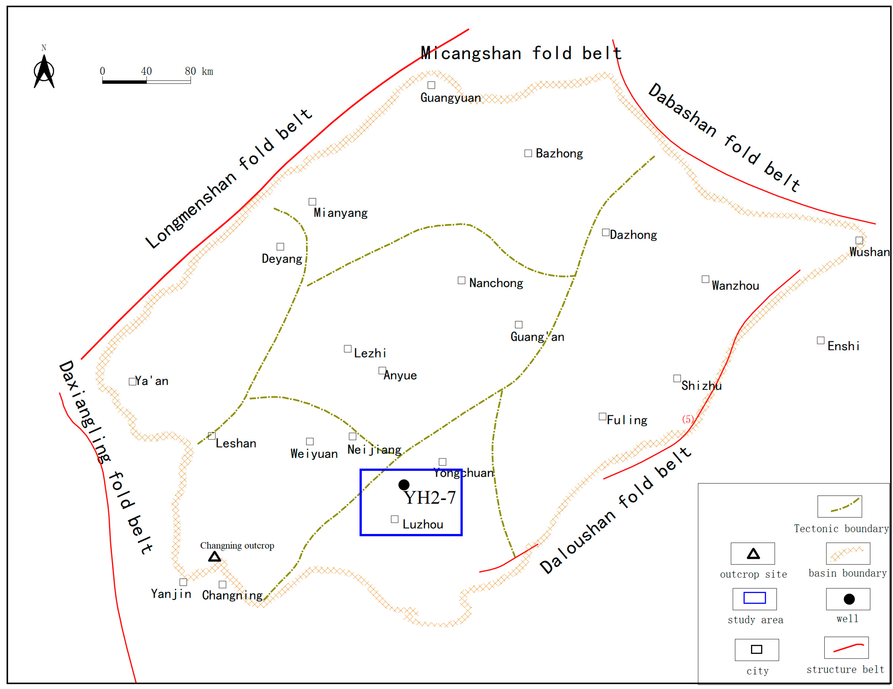
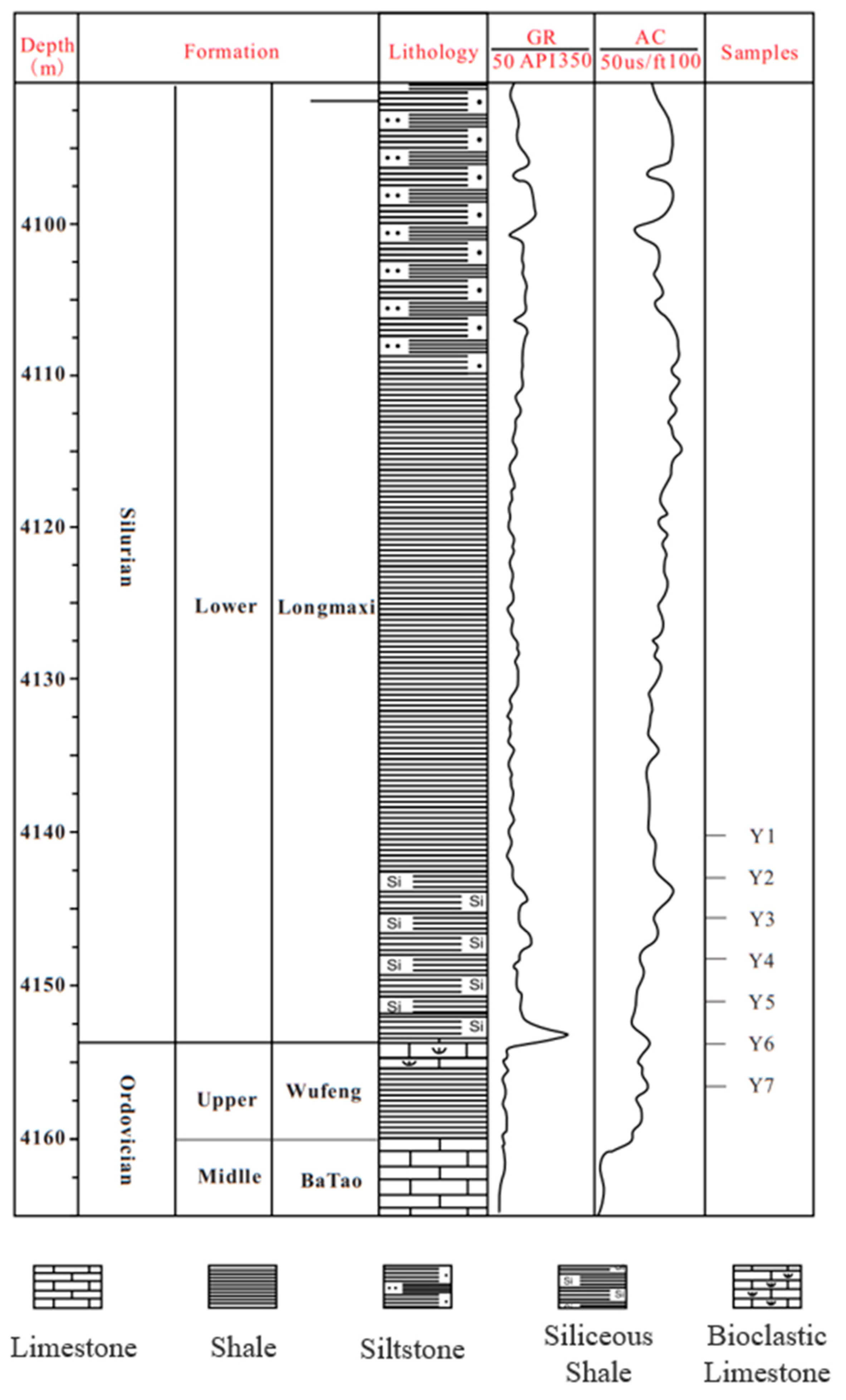
2.1. Samples

The deep shale samples were obtained from the sub-4000 m buried reservoir in the Luzhou Block in the southern Sichuan Basin, China (Figure 1). The Luzhou block is located in the south Sichuan low fold belt, between the south slope of the middle Sichuan ancient uplift and the southeast Sichuan depression fold belt. The stratigraphic sequence in the area is normal and the Jurassic strata are mainly exposed at the surface, while the Upper Triassic Xujiahe Formation is exposed on the top of some back-sloping structures. The depth of the burial of strata at the bottom of the Wufeng Formation–Longmaxi Formation in the study area ranges from 3500–4500 m. Black carbonaceous shale is developed at the bottom of the Longmaxi Formation and graptolite and pyrite are common in the cross-section.
According to the lithology and logging response characteristics (Figure 2), the Longmaxi Formation can be subdivided into the sections Long 1 and Long 2. Section Long 1 is well preserved in the Luzhou Block, with a thickness of 441–575 m. The regional distribution is stable and comparable. Based on the lithology, stratigraphy and electrical properties, section Long 1 can be further divided into Long 1 Subsection 1 and Long 1 Subsection 2 from the bottom up. Subsection 1 is a set of organic-rich black carbonaceous shales, with different morphological graptolites, phyllite development, pyrite-rich nodules, and pyrite-filled horizontal joints. The thickness ranges from 31 to 74 m, averaging 55 m, which is greater than that of Changning (40 m) and Weiyuan (48 m), and with general thickening in the southeast direction. According to the lithological, sedimentary tectonic, paleontological, and electrical data, Subsection 1 can be further divided into four categories: L111, L112, L113 and L114. The current shale gas production and the samples mainly originate from Long 1 Subsection 1 and the Wufeng Formation. Shallow samples from the Weiyuan block in southern Sichuan were compared, which were buried at 2500–2600 m and obtained from the Long Yi 1 Subsection and Wufeng Formation. Table 1 lists the basic geological information and lithofacies of all of the samples. Furthermore, the shale lithofacies were classified based on their organic matter richness and mineral compositions [30]. According to the mineral compositions, the lithofacies of the shale samples were classified into three main types: siliceous shale lithofacies (S), calcareous/siliceous mixed shale lithofacies (CS), and calcareous shale lithofacies (C).
In this experiment, seven deep shale samples from the Luzhou Block and three shallow samples from the Weiyuan Block were ground and screened in order to obtain four groups of crushed samples with different particle diameters of 20–40, 40–80, 100–160 and 200–400 mesh. To eliminate the residual bound water and capillary moisture in the samples, the samples were dried at 105 °C for 24 h. The samples were first degassed under a vacuum at 105 °C for 12 h in order to remove the air and water from the pores. Later, the nitrogen adsorption and desorption curves of the shale samples with different particle diameters were obtained experimentally. The equilibrium time was set to 10 s during the measurements.

2.2. Low Temperature Nitrogen Adsorption Experiment

Samples were analyzed using a Micromeritics ASAP 2420 specific surface area and porosity analyzer and the equilibration time was set to 10 s [31]. The instrument has a pore size measurement range from 0.35 to 400 nm, adsorption–desorption relative pressure ranges between 0.004–0.995, 0.005 m2/g surface area, and 0.0001 cm3/g pore volume.
The adsorption amount of nitrogen in the medium at equilibrium was measured by gradually increasing/decreasing the relative pressure (P/P0, where P is the partial pressure of nitrogen and P0 is the saturation vapor pressure of nitrogen at the critical temperature). The critical temperature was 195.8 °C and high-purity nitrogen (>99.999%) was employed as the adsorbent. Subsequently, the adsorption–desorption curve was obtained and used to characterize the pore size and specific surface area distribution of the medium. When the relative pressure was low (<0.35), the nitrogen was mainly adsorbed onto micropores and mesopores. Monomolecular layer adsorption and micropore filling are the main micropore mechanisms, while monomolecular layer adsorption is the main mesopore mechanism. When the relative pressure value increased (>0.4), capillary coalescence occurred in the mesopores and macropores. According to Kelvin’s theory, the larger the relative pressure value is, the larger the pore size is at the capillary coalescence, so the pore capacity and pore size distribution can be calculated based on the adsorption curve. The common pore size characterization methods are the Barrett–Joyner–Halenda (BJH) [32] and density–functional theory (DFT) [33] models. The BJH method is based on the Kelvin equation, which is not applicable to pores measuring <7 nm and needs to be corrected. The DFT method is based on the global density distribution function, portraying the distribution of micropores, mesopores and some macropores. In this study, the DFT model was selected for the pore size distribution calculation and the effective pore size interval ranged from 1.48 to 117.00 nm [34].

3. Results and Discussion

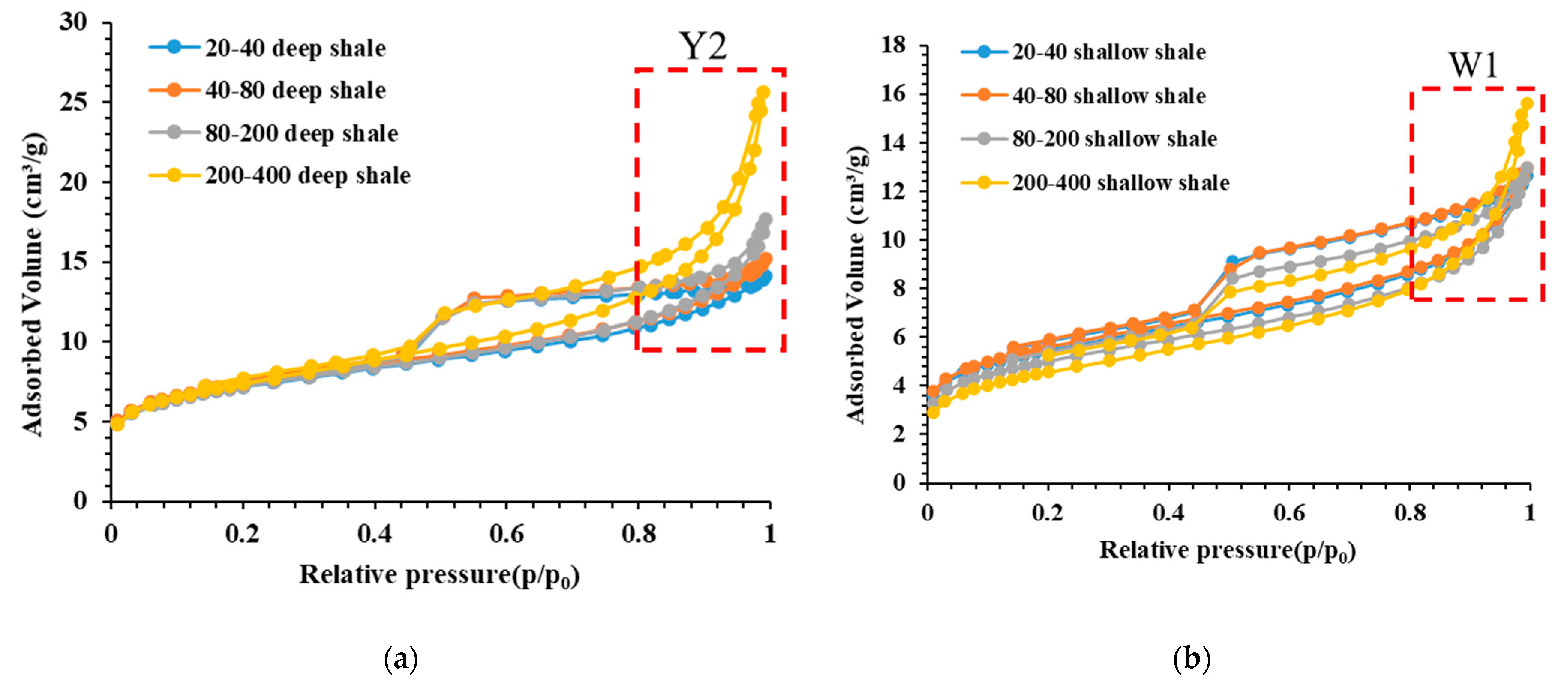
3.1. Adsorption–Desorption Curve Characteristics

The test results of the deep layer Y2 and shallow layer W1 samples are considered as examples and their low-pressure N2 isothermal adsorption–desorption curves are shown in Figure 3.
As shown in Figure 3, in the relative pressure range of 0.5–1, the low-temperature nitrogen adsorption and desorption processes of the shale samples did not overlap. The desorption line is located above the adsorption line, forming an obvious hysteresis loop. Furthermore, all of the curves are similar to the IV isothermal adsorption curve that is recommended by the International Union of Pure and Applied Chemistry (IUPAC) [35], with the hysteresis loop appearing between H3 and H4. The appearance of a hysteresis loop is closely related to the pore structure of the shale. When nitrogen capillary condensation occurs, it starts from the liquid surface of the annular adsorption film on the wall of the hole and the desorption starts from the spherical meniscus of the hole. Therefore, the shape of the hysteresis loop can reflect the pore shape and connectivity qualitatively.
When the relative pressure was close to 1, none of the samples showed a “plateau”. This meant that they did not reach saturation, indicating that, in addition to micropores and mesopores, macropores larger than 200 nm had developed in the experimental samples. All of the samples showed that the adsorption curves in the high-pressure section steepened with decreasing particle size and the maximum adsorption volume of the 200–400 mesh samples was 1.62 times that of the 20–40 mesh samples on average, indicating that the increase in adsorption sites as particle size decreased was not only related to the newly created particle surface, but may have led to the connection of some unconnected large pores of the shale with the outside world.
The isothermal adsorption curves with relative pressure P/P0 values ranging from 0.8 to 1 were further analyzed; the adsorption curves corresponded to the large pore size pore regions [36]. As shown in Figure 4, there was no significant correlation between the increase in the nitrogen adsorption capacity and the TOC in all of the samples at a relative pressure of 0.8–1. Thus, the macropores of this experimental sample were not dominated by organic matter pores. However, certain scholars have compared the adsorption capacity of different particle sizes with the sample TOC and found that the maximum adsorption capacity of the samples increased rapidly with the increase in particle size at a higher TOC content [37]. Collectively, the macropore types within the different samples varied, which warrants a separate discussion.
Further analysis of the change in the adsorption capacity showed that the increase in the adsorption capacity mainly occurred at relatively high pressures, which also indicated that larger pores were related to the decrease in particle size. This phenomenon is quantitatively analyzed below.

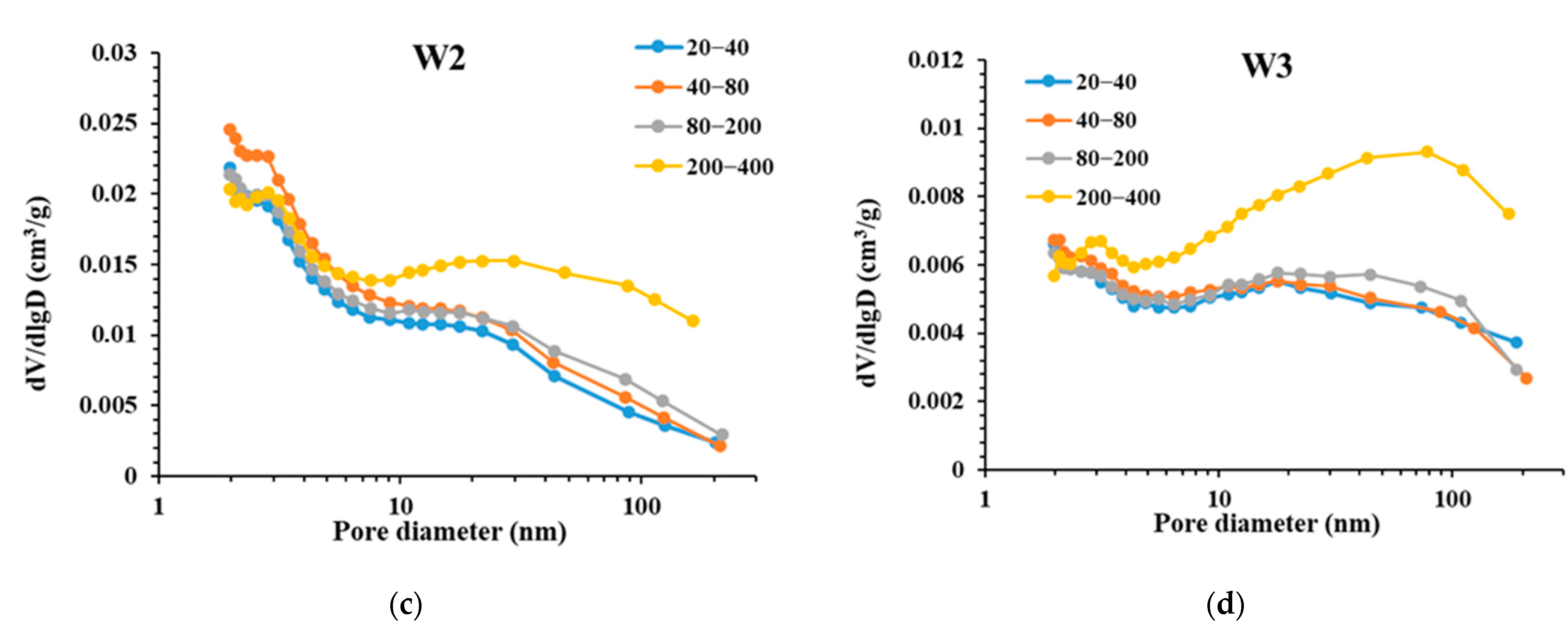
3.2. Comparative Analysis of Pore Volume

The LTNA interpretation results are shown in Figure 3 and Table 2, including the pore volume, specific surface area, and pore content of the shale in different intervals.
According to the variation law of the pore distribution of samples with different particle sizes, this study divided the pore interval into three parts: interval A (2–5 nm: small mesopores), interval B (5–20 nm: medium mesopores) and interval C (>20 nm: large mesopores and macropores). The pores in intervals A, B and C are referred to as small pores, medium pores and large pores, respectively. The following analysis shows that the samples that were used in the present experiment developed pores below 5 nm and that the pores above 20 nm were greatly affected by the pore size. Therefore, the pores were divided into three categories based between 5 nm and 20 nm.
As shown in Figure 5, the pore volumes of the shale samples with different particle sizes varied significantly. The average pore volume of all of the samples with 200–400 mesh was 175.84% of the 20–40 mesh. Among them, the largest change was found in the pore volume of sample Y7, which increased by 96%, while the pore volume of sample W1 had the smallest increase of 30%. There was no significant difference in the shale pore volume within the grid ranges of 20–40, 40–80, and 100–160, and the average growth rate was only 15.11%. This is far less than the average pore volume growth rate of the 200–400 mesh samples, by 75.85%. Among the two groups of the Y7 and W1 samples, the measured pore volume of the 100–160 mesh samples were smaller than that of the 40–80 mesh samples, which is likely to be because the sample fragmentation process not only connected the isolated pores, but also possibly destroyed some existing pores.
Figure 5 shows the density functional theory (DFT) pore size distribution of typical shale samples with different grain sizes. The pore size distribution of all of the samples with different particle sizes had obvious inheritance and similar curve patterns. The pore volume of the deep shale sample was mainly concentrated in interval A and interval B. This is because deep shale is subjected to strong mechanical compaction and small pores have a stronger compressive test ability.
As shown in Figure 6, with the decrease in the particle size, the pore volumes of interval A and interval B changed only slightly. This may be due to the fact that the pore throats between small-aperture pores are more likely to be destroyed during the sample crushing process, which reduces the connectivity between pores. This leads to the volume of the newly connected pores and the volume of the damaged pores offsetting each other. Therefore, the pore volume of interval A and interval B showed no obvious change. However, the pore volume in the C region increased rapidly from 0.00359 cm3/g to 0.01464 cm3/g. This indicates that a large number of large pores in the shale were isolated pores. Large pores find it easier to communicate as the particle size decreases. In the reservoir environment, the gas pressure was significantly higher than that which was found in the LTNA experiment, so the pores that were not connected for the nitrogen adsorption experiment should be connected in the actual reservoir environment. Therefore, in order to characterize shale’s pore structure more comprehensively, shale samples with smaller particle sizes should be selected. However, with the deepening of the crushing effect, more artificial secondary fractures will be generated, changing the pore structure of the shale. Therefore, the application of the 120–160 mesh samples in the calculation of the pore volume is recommended.

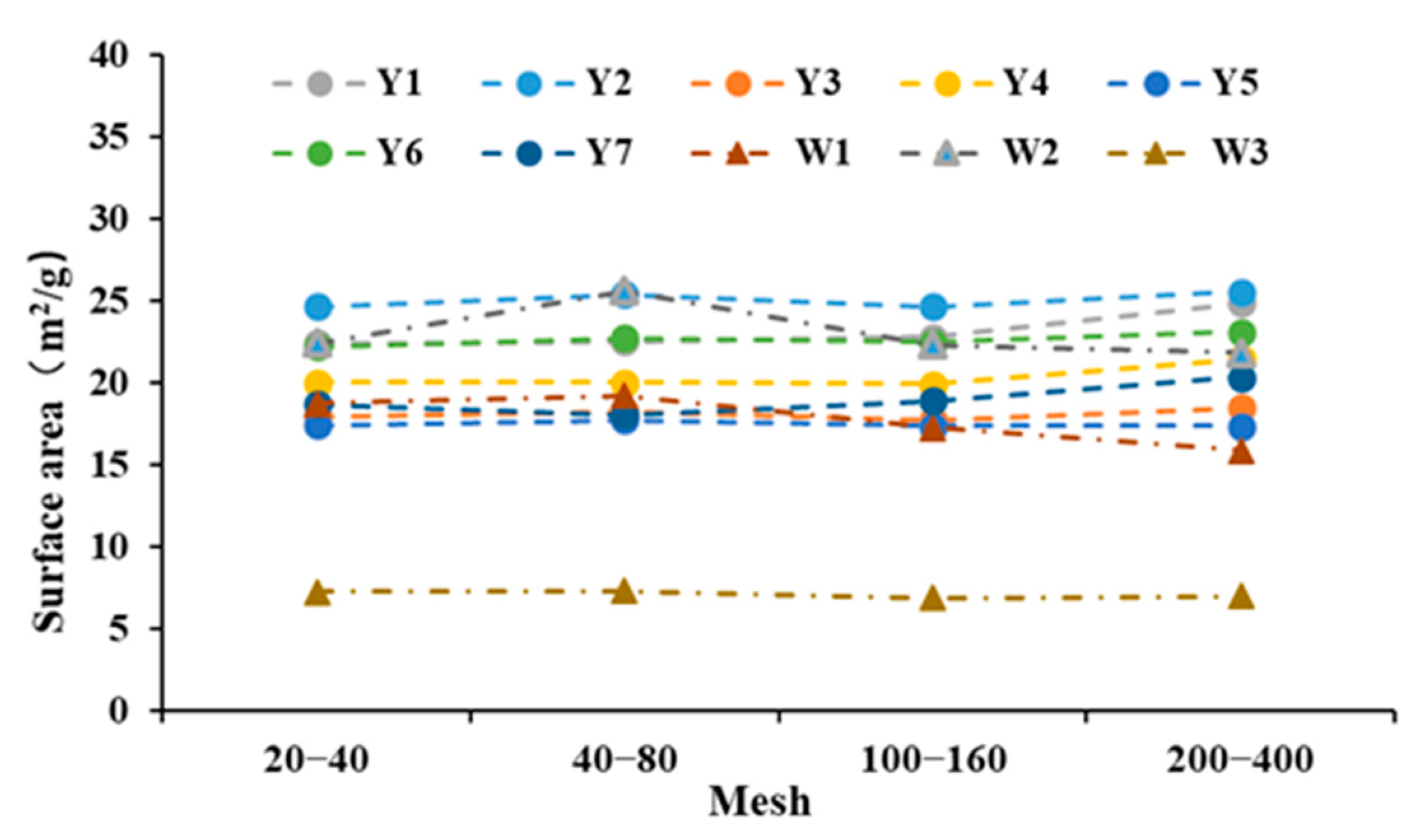
3.3. Specific Surface Area Analysis

Figure 7 shows the specific surface area of the samples.
As shown in Figure 7, the specific surface areas of all of the samples in this experiment were almost unaffected by the particle size. The largest rate of change was observed in the W11 sample, with a rate of change of only 14%. The pore size distribution of the specific surface area of the typical samples is shown in the figure below, where most of the specific surface area constitutes intervals A and B; 76.43% of which is interval A, 19.93% interval B, and 3.63% interval C, for the 20–40 mesh samples. Further, for the 40–80 mesh samples, 75.71% was covered by interval A, 20.17% constituted interval B, and only 4.17% constituted interval C. For the 80–200 mesh samples, 74.11% constituted the pores in interval A, 20.89% the pores in interval B, and only 5.00% those in interval C, whereas 67.23% constituted the pores in interval A and 67.23% the pores in interval B for the 200–400 mesh samples.
As shown in Figure 8, the percentage of the specific surface area that was covered by the 200–400 mesh sample was 67.23% in interval A, 23.96% in interval B, and 8.79% in interval C. The experiments showed that the specific surface area of the samples did not change significantly across the four particle sizes and only a small decrease in the percentage of interval A occurred in the 200–400 mesh samples. This was because, as the particle size decreased, the number of pores in interval B that communicated with the pores in interval C increased and the percentage of the C interval that was under all of the mesh sizes was below 10%. Therefore, the pores in area A were the main contributors to the specific surface area of this sample. Based on the analysis in the previous section, the pores were not significantly affected by the particle size of the samples. Therefore, the specific surface area and the pore size of the samples did not change significantly with the particle size. Therefore, there is no special requirement for sample mesh size when studying the specific surface area of shale by nitrogen adsorption.

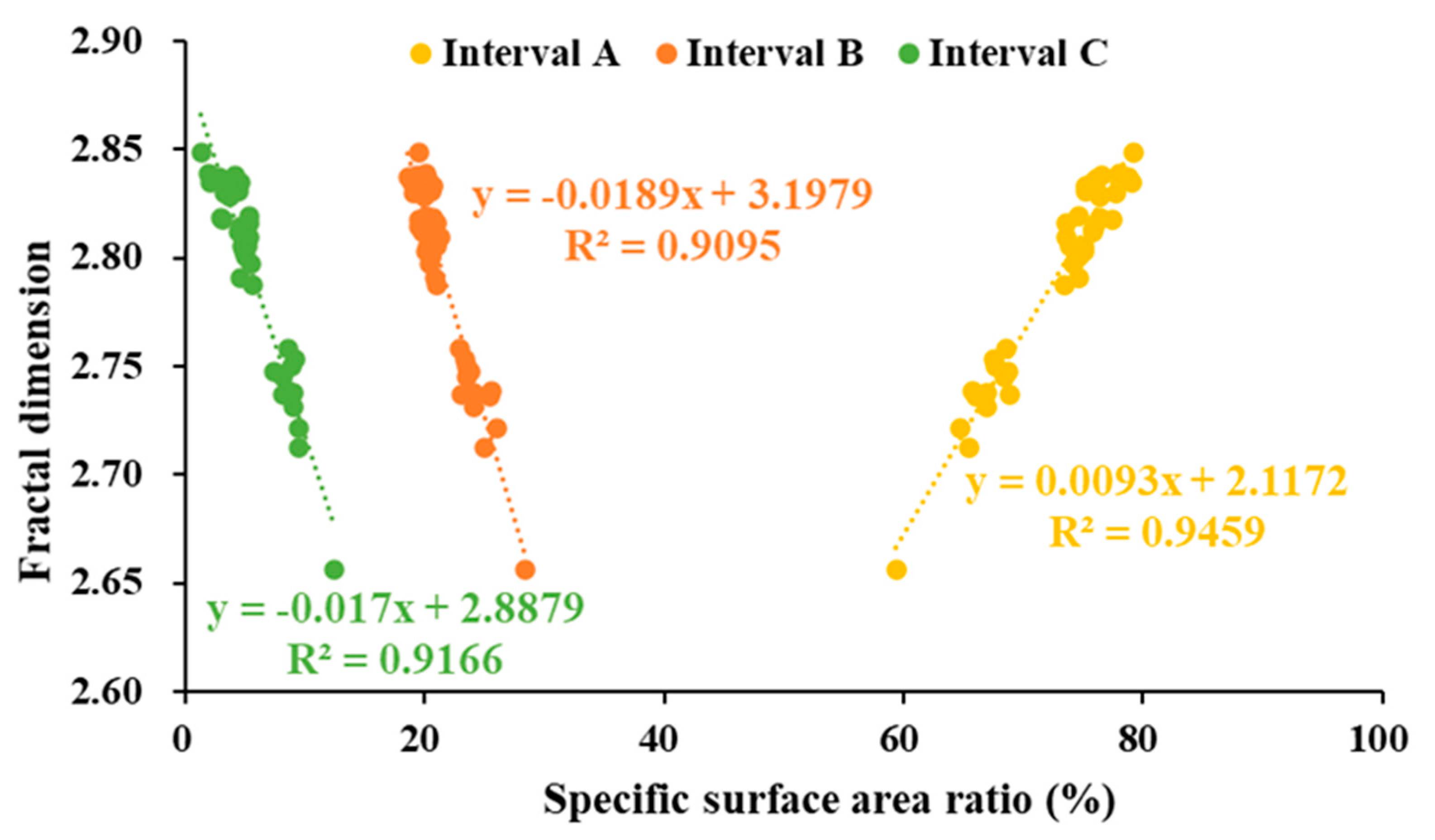
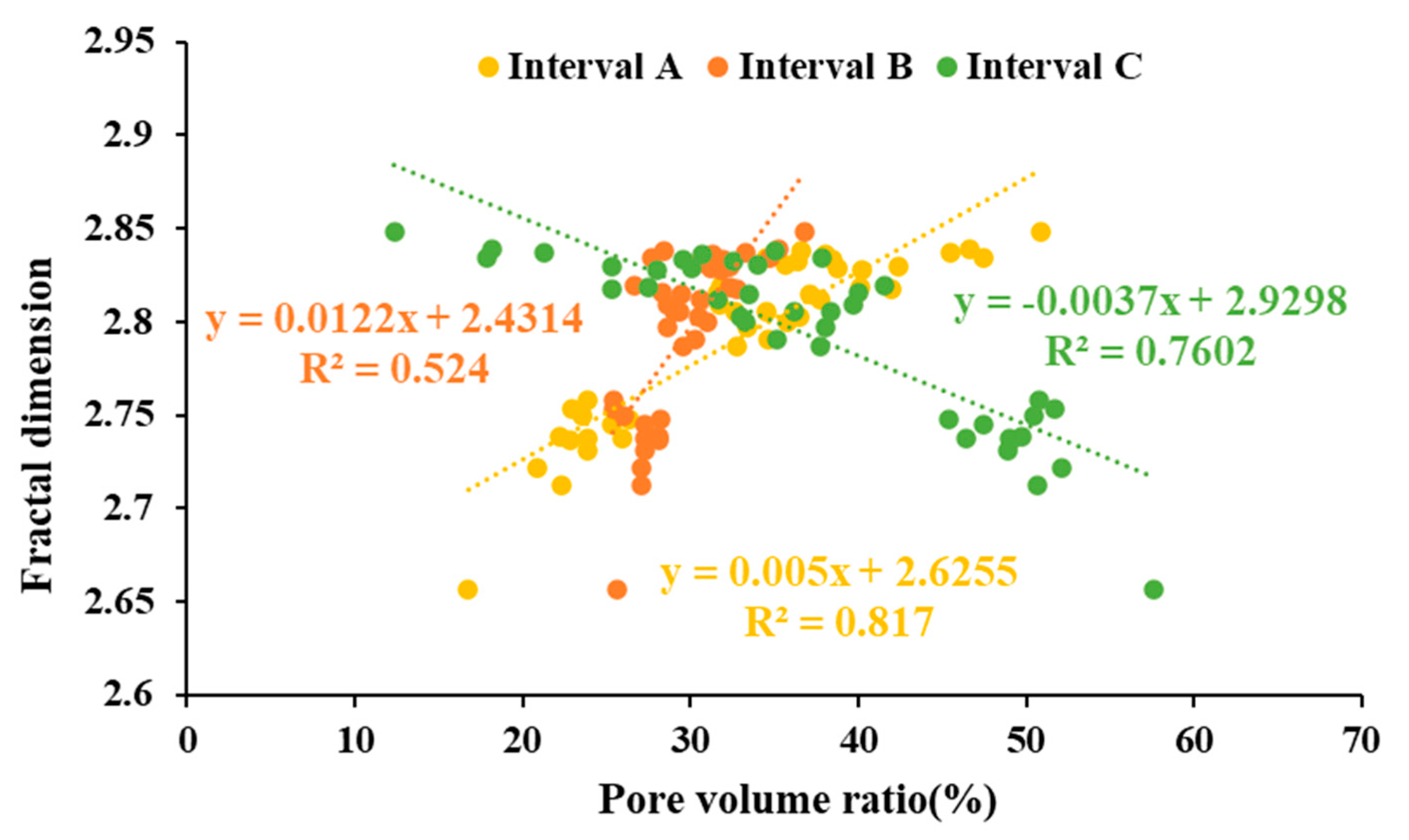
3.4. Comparative Analysis of the Fractal Dimension

Based on the nitrogen adsorption data, Pfeifer’s Frenkel–Halsey–Hill (FHH) model (Equation (1)) was used in order to calculate the fractal dimension of the shale. The fractal dimension is usually 2–3. When the value of the fractal dimension is close to 2, the solid surface is smooth and homogeneous, whereas a value close to 3 reflects a complex pore structure with an extremely irregular and non-homogeneous pore surface and high resistance to fluid flow [5,38].
l n ( V V 0 ) = K [ l n [ l n p 0 p ] ] + C
where V is the adsorption volume of the sample gas at equilibrium pressure (cm3/g), V0 is the monolayer coverage volume (cm3/g), P0 is the saturation vapor pressure of the adsorbed gas (MPa), P is the equilibrium pressure of the system (MPa), K is the slope of the fitted line and is related to the adsorption mechanism, and C is a constant. When the adsorption mechanism is capillary condensation, D = K + 3 and D is the fractal dimension. When the adsorption mechanism is van der Waals and capillary action is not considered, according to the literature [39,40], D = 3K + 3. If the reservoir pores have fractal characteristics, l n ( V V 0 ) has a linear relationship with l n p 0 p according to slope K and this can be used to calculate the fractal dimension D.
In this study, the samples all showed adsorption hysteresis loops (Figure 3) when the relative pressure exceeded 0.45. The isothermal adsorption line branches and desorption branches obviously did not overlap and capillary condensation occurred for the nitrogen adsorption. Therefore, D = K + 3 was selected for the calculation.
The fractal dimension of all of the samples is shown in Table 3.
As shown in Figure 9, the average pore volume fractal dimension was 2.82 for the sample sizes ranging from 20–40 mesh, 2.81 for those ranging from 40–80 mesh, 2.79 for those ranging from 80–200 mesh, and 2.73 for the 200–400 mesh sample sizes. The pore volume fractal dimension of almost all of the samples decreased as the particle size decreased, indicating that the irregularity of the shale pore surface decreases as the particle size decreases. The fractal dimensions of the shallow and deep samples were significantly smaller than those of the deep samples, which suggested that the deep samples had a more complex pore structure than the shallow samples (Figure 9).
As shown in Figure 10, the relationship between the specific surface area percentage and the fractal dimension of regions A, B, and C were analyzed. The fractal dimension was highly positively correlated with the fractal dimension percentage of the small pore region, with a correlation coefficient R2 of 0.95; however, it had a high negative correlation with the medium and large pore contents, with a correlation coefficient R2 of 0.92 and 0.91.
The fractal dimension of shale is considered to be related to the distribution of the specific surface area of differently sized pores. When the ratio of the total specific surface area that is occupied by micropores increases (i.e., the ratio of the specific surface area occupied by medium and large pores is smaller), the fractal dimension of the shale increases holistically. The reason for this may be that the larger the specific surface area is, the greater the surface area of the shale in unit volume is, and the shale is more likely to have a complex structure and be rougher, so the fractal dimension of the shale is larger. The pore-specific surface area is the subject contributor to the specific surface area, so the higher the pore content is, the greater the fractal dimension will be.
Subsequently, the samples from different layers with the same particle size in the same well were compared. The fractal dimension of the samples of each layer was found to not be significantly different nor uniform, but there was a certain gap between the different wells. It showed that the geological tectonic movement in the same well was similar and there was no significant difference in the complexity of the pores.
As shown in Figure 11, by further analysis of the regional pore volume ratio, the fractal dimension was found to be highly positively correlated with the small pore content. The small pore content yielded a correlation coefficient R2 equals 0.82; the medium pore content a correlation coefficient R2 equals 0.52; and the large pore content a correlation coefficient R2 equals 0.76. This indicates that the fractal dimension is mainly controlled by the development degree of the small and large pores. Greater development of small pores and the less development of large pores correlates with a larger fractal dimension and a more complex internal structure of the samples. This can be attributed to the fact that the pore structure of the small pores is more complex than that of the medium and large pores. This also indicates that the fractal dimension of the samples decreases as the particle size decreases, because more large pores appear when the particle size decreases. Therefore, the decrease in the proportion of the pores leads to a decrease in the fractal dimension of the sample.
The fractal dimension of the samples, the pore volume and the specific surface area have been analyzed [41] and it has been concluded that the fractal dimension, pore volume, and specific surface area values are correlated. This is because the fractal dimension reflects the overall complexity of the sample. For example, when the pore volume of the sample increases, the overall pore content of each part of the sample does not change; if the pore volume of mesopores and macropores increases proportionally, the overall complexity does not increase. Therefore, the fractal dimension of the sample is related to the relative content, but not to the absolute content of the pores. There was no significant relationship with the absolute content of the pores.
As shown in Figure 12, the correlation coefficients, R2, of the fractal dimensions of the samples with different particle diameters in the same group were 0.889 for the 20–40 mesh samples, 0.922 for 40–80 mesh samples, 0.953 for the 160–200 mesh samples, and 0.991 for the 200–400 mesh samples. The correlation coefficients of the fractal dimensions of almost all of the experimental samples increased as their particle size decreased, indicating that the samples showed stronger fractal characteristics as the particle size decreased. Therefore, 200–400 mesh size samples are recommended in the study of the fractal characteristics of deep shale via nitrogen adsorption.

4. Conclusions

In this study, the effects of different particle sizes in deep shale samples on nitrogen adsorption results were analyzed.
  • Grain size has a great effect on pore volume and pore distribution measurements. The total shale pore volume measurements showed a small increase followed by a large increase as the grain size decreases, which is not significantly related to TOC.
  • The particle size exerts a certain influence on the accuracy of the fractal dimension and the correlation coefficient of the fractal dimension increases significantly as the particle size of the sample decreases. Furthermore, the complexity of the pore structure of deep samples is influenced by more controlling factors. The use of 200–400 mesh size samples is recommended when studying fractal dimensions.
  • The micropores and small mesopores (<20 nm) of the shale samples provide many pore volumes and this intensifies with increasing burial depth. Isolated pores are developed in larger mesopores and macropores (>20 nm) and further analysis is needed under reservoir conditions.
  • The specific surface area of shale is almost unaffected by the particles’ size. The surface area’s size is mainly controlled by the micropores and small pore size mesopores. The specific surface area of the small pores contributes most of the total specific surface area of deep shale samples.
  • There are different requirements for the sample mesh for the study of different shale characteristics by nitrogen adsorption. Among them, 120~160 mesh size samples are recommended for the study of pore volume, and 200~400 mesh size samples are recommended for the study of the fractal dimension. The study of specific surface area grid samples has no specific grid requirements.

Author Contributions

Conceptualization, H.Z. and Y.L.; methodology, Y.L.; validation, Z.H. and X.D.; formal analysis, H.Z.; investigation, Y.L.; resources, X.L.; data curation, X.L.; writing—original draft preparation, X.L.; writing—review and editing, H.Z.; visualization, W.G.; supervision, Z.H.; project administration, Z.H.; funding acquisition, H.Z. All authors have read and agreed to the published version of the manuscript.

Funding

This research was funded by the Demonstration Project of the National Science and Technology Major Project of the Ministry of Science and Technology of China, grant number No. 2016ZX05062-002-001.

Data Availability Statement

The data presented in this study are available on request from the corresponding author. The data are not publicly available due to some data confidentiality restrictions.

Conflicts of Interest

The authors declare no conflict of interest.

References

  1. Vidic, R.D.; Brantley, S.L.; Vandenbossche, J.M.; Yoxtheimer, D.; Abad, J.D. Impact of shale gas development on regional water quality. Science 2013, 340, 1235009. [Google Scholar] [CrossRef] [PubMed] [Green Version]
  2. Zhang, L.H.; He, X.; Li, X.G.; Li, K.C.; He, J.; Zhang, Z.; Guo, J.J.; Chen, Y.N.; Liu, W.S. Shale gas exploration and development in the Sichuan Basin: Progress, challenge and countermeasures. Nat. Gas Ind. 2021, 41, 143–152. [Google Scholar]
  3. Ma, X.H.; Li, X.Z.; Liang, F.; Wan, Y.J.; Shi, Q.; Wang, Y.H.; Zhang, X.W.; Che, M.G.; Guo, W. Dominating factors on well productivity and development strategies optimization in Weiyuan shale gas play, Sichuan Basin, SW China. Pet. Explor. Dev. 2020, 47, 594–602. [Google Scholar] [CrossRef]
  4. Li, X.Z.; Guo, Z.H.; Hu, Y.; Liu, X.H.; Wan, Y.J.; Luo, R.L.; Sun, Y.P.; Che, M.G. High-quality development of ultra-deep large gas fields in China: Challenges, strategies and proposals. Nat. Gas Ind. 2020, 40, 75–82. [Google Scholar] [CrossRef]
  5. Liu, S.G.; Deng, B.; Zhong, Y.; Ran, B.; Yong, Z.Q.; Sun, W.; Yang, D.; Jiang, L.; Ye, Y.H. Unique geological features of burial and superimposition of the Lower Paleozoic shale gas across the Sichuan Basin and its periphery. Earth Sci. Front. 2016, 23, 11–28. [Google Scholar]
  6. Nie, H.K.; Bian, R.K.; Zhang, P.X.; Gao, B. Micro-types and characteristics of shale reservoir of the lower paleozoic in southeast Sichuan basin, and their effects on the gas content. Earth Sci. Front. 2014, 21, 331–343. [Google Scholar]
  7. Chen, Y.; Wei, L.; Mastalerz, M.; Schimmelmann, A. The effect of analytical particle size on gas adsorption porosimetry of shale. Int. J. Coal Geol. 2015, 138, 103–112. [Google Scholar] [CrossRef] [Green Version]
  8. Alsalem, O.B.; Fan, M.; Xie, X. Late Paleozoic subsidence and burial history of the Fort Worth basin. AAPG Bull. 2017, 101, 1813–1833. [Google Scholar] [CrossRef]
  9. Hao, F.; Zou, H.Y.; Lu, Y.C. Mechanisms of shale gas storage: Implications for shale gas exploration in China. AAPG Bull. 2013, 97, 1325–1346. [Google Scholar] [CrossRef]
  10. Hou, B.; Diao, C.; Li, D.D. An experimental investigation of geomechanical properties of deep tight gas reservoirs. J. Nat. Gas Sci. Eng. 2017, 47, 22–33. [Google Scholar] [CrossRef]
  11. Guan, Q.Z.; Dong, D.Z.; Lu, H.; Liu, B. Influences of abnormal high pressure on Longmaxi shale gas reservoir in Sichuan Basin. Xinjiang Pet. Geol. 2015, 36, 55–60. [Google Scholar]
  12. Anovitz, L.M.; Cole, D.R. Characterization and analysis of porosity and pore structures. Rev. Mineral. Geochem. 2015, 80, 61–164. [Google Scholar] [CrossRef] [Green Version]
  13. Loucks, R.G.; Reed, R.M. Abstract: Scanning-electron-microscope petrographic evidence for distinguishing organic-matter pores associated with depositional organic matter versus migrated organic matter in mudrocks. Gcags Trans. 2014, 3, 51–60. [Google Scholar]
  14. Liu, W.B.; Zhang, S.Q.; Li, S.Z.; Zhou, X.G.; Wang, D.D.; Zhang, W.H.; Lin, Y.H. Development characteristics and geological significance of microfractures in the Es3 reservoirs of Dongpu depression. Geol. Bull. China 2018, 37, 496–502. [Google Scholar]
  15. Lin, W.; Xiong, S.C.; Liu, Y.; He, Y.; Chu, S.S.; Liu, S.Y. Spontaneous imbibition in tight porous media with different wettability: Pore-scale simulation. Phys. Fluids 2021, 33, 032013. [Google Scholar] [CrossRef]
  16. Sun, J.M.; Dong, X.; Wang, J.J.; Schmitt, D.R.; Xu, C.L.; Mohammed, T.; Chen, D.W. Measurement of total porosity for gas shales by gas injection porosimetry (GIP) method. Fuel 2016, 186, 694–707. [Google Scholar] [CrossRef]
  17. Hu, H.Y.; Zhang, T.W.; Wiggins-Camacho, J.D.; Ellis, G.S.; Lewan, M.D.; Zhang, X.L. Experimental investigation of changes in methane adsorption of bitumen-free Woodford Shale with thermal maturation induced by hydrous pyrolysis. Mar. Pet. Geol. 2015, 59, 114–128. [Google Scholar] [CrossRef]
  18. Yang, F.; Ning, Z.F.; Kong, D.T.; Liu, H.Q. Pore structure of shale from high pressure mercury injection and nitrogen adsorption method. Nat. Gas Geosci. 2013, 24, 450–455. [Google Scholar]
  19. Ramirez, T.R.; Klein, J.D.; Ron, J.M.; Howard, J.J. Comparative study of formation evaluation methods for unconventional shale gas reservoirs: Application to the Haynesville shale (Texas). In Proceedings of the SPE North American Unconventional Gas Conference and Exhibition, The Woodlands, TX, USA, 14–16 June 2011. [Google Scholar]
  20. Xu, H.; Tang, D.Z.; Zhao, J.L.; Li, S. A precise measurement method for shale porosity with low-field nuclear magnetic resonance: A case study of the Carboniferous–Permian strata in the Linxing area, eastern Ordos Basin, China. Fuel 2015, 143, 47–54. [Google Scholar] [CrossRef]
  21. Yang, F.; Ning, Z.F.; Liu, H.Q. Fractal characteristics of shales from a shale gas reservoir in the Sichuan Basin, China. Fuel 2014, 115, 378–384. [Google Scholar] [CrossRef]
  22. Hinai, A.A.; Rezaee, R.; Esteban, L.; Labani, M. Comparisons of pore size distribution: A case from the Western Australian gas shale formations. J. Unconv. Oil Gas Resour. 2014, 8, 1–13. [Google Scholar] [CrossRef]
  23. Yin, L.L.; Guo, S. Full-sized pore structure and fractal characteristics of marine-continental transitional shale: A case study in Qinshui basin, North China. Acta Geol. Sin. 2019, 93, 675–691. [Google Scholar] [CrossRef]
  24. Wei, M.M.; Xiong, Y.Q.; Zhang, L.; Li, J.H.; Peng, P.A. The effect of sample particle size on the determination of pore structure parameters in shales. Int. J. Coal Geol. 2016, 163, 177–185. [Google Scholar] [CrossRef]
  25. Li, J.; Zhou, S.X.; Fu, D.L.; Li, Y.J.; Ma, Y.; Yang, Y.N.; Li, C.C. Changes in the pore characteristics of shale during comminution. Energy Explor. Exploit. 2016, 34, 676–688. [Google Scholar] [CrossRef] [Green Version]
  26. Han, H.; Cao, Y.; Chen, S.J.; Lu, J.G.; Huang, C.X.; Zhu, H.H.; Zhan, P.; Gao, Y. Influence of particle size on gas-adsorption experiments of shales: An example from a Longmaxi Shale sample from the Sichuan Basin, China. Fuel 2016, 186, 750–757. [Google Scholar] [CrossRef] [Green Version]
  27. Mastalerz, M.; Hampton, L.; Drobniak, A.; Loope, H. Significance of analytical particle size in low-pressure N2 and CO2 ad-sorption of coal and shale. Int. J. Coal Geol. 2017, 178, 122–131. [Google Scholar] [CrossRef]
  28. Jiao, K.; Ye, Y.H.; Liu, S.G.; Ran, B.; Deng, B.; Li, Z.W.; Li, J.X.; Yong, Z.Q.; Jiang, L.; Xia, G.D.; et al. Nanopore characteristics of super-deep buried mudstones in Sichuan Basin and its geological implication. J. Chengdu Univ. Technol. Sci. Technol. Ed. 2017, 44, 129–138. [Google Scholar] [CrossRef]
  29. He, Z.L.; Nie, H.K. Geological problems in the effective development of deep shale gas taking Sichuan Basin and its surrounding Wufeng Formation-Longmaxi Formation as an example. Acta Pet. Sin. 2020, 41, 379–391. [Google Scholar]
  30. Yang, F.; Xu, S.; Hao, F.; Hu, B.Y.; Zhang, B.Q.; Shu, Z.G.; Long, S.Y. Petrophysical characteristics of shales with different lithofacies in Jiaoshiba area, Sichuan Basin, China: Implications for shale gas accumulation mechanism. Mar. Pet. Geol. 2019, 109, 394–407. [Google Scholar] [CrossRef]
  31. Yang, F.; Xie, C.; Ning, Z.F.; Krooss, B.M. High-pressure methane sorption on dry and moisture-equilibrated shales. Energy Fuels 2017, 31, 482–492. [Google Scholar] [CrossRef]
  32. Barrett, E.P.; Joyner, L.G.; Halenda, P.P. The determination of pore volume and area distributions in porous substances. I. Computations from nitrogen isotherms. J. Am. Chem. Soc. 1951, 73, 373–380. [Google Scholar] [CrossRef]
  33. Thommes, M. Physical adsorption characterization of nanoporous materials. Chem. Ing. Tech. 2010, 82, 1059–1073. [Google Scholar] [CrossRef]
  34. Li, B.; Chen, F.W.; Xiao, D.S.; Lu, S.F.; Zhang, L.C.; Zhang, Y.Y.; Gong, C. Effect of particle size on the experiment of low temperature nitrogen adsorption: A case study of marine gas shale in Wufeng-Longmaxi formation. J. China Univ. Min. Technol. 2019, 48, 395–404. [Google Scholar] [CrossRef]
  35. Thommes, M.; Kaneko, K.; Neimark, A.V.; Olivier, J.P.; Rodriguez-Reinoso, F.; Rouquerol, J.; Sing, K.S.W. Physisorption of gases, with special reference to the evaluation of surface area and pore size distribution (IUPAC Technical Report). Pure Appl. Chem. 2015, 87, 1051–1069. [Google Scholar] [CrossRef] [Green Version]
  36. Xie, X.Y.; Tang, H.M.; Wang, C. Comparison of nitrogen adsorption method and mercury injection method in testing pore size distribution of shale. Nat. Gas Ind. 2006, 26, 100–102. [Google Scholar] [CrossRef]
  37. Liu, X.J.; Xiong, J.; Liang, L.X. Investigation of pore structure and fractal characteristics of organic-rich Yanchang formation shale in central China by nitrogen adsorption/desorption analysis. J. Nat. Gas Sci. Eng. 2015, 22, 62–72. [Google Scholar] [CrossRef]
  38. Lin, W.; Li, X.Z.; Yang, Z.M.; Lin, L.J.; Xiong, S.C.; Wang, Z.Y.; Wang, X.Y.; Xiao, Q.H. A new improved threshold segmentation method for scanning images of reservoir rocks considering pore fractal characteristics. Fractals 2018, 26, 1840003. [Google Scholar] [CrossRef] [Green Version]
  39. Xie, D.L.; Guo, Y.H.; Zhao, D.F. Fractal characteristics of adsorption pore of shale based on low temperature nitrogen experiment. J. China Coal Soc. 2014, 39, 2466–2472. [Google Scholar]
  40. Pfeifer, P.; Wu, Y.J.; Cole, M.W.; Krim, J. Multilayer adsorption on a fractally rough surface. Phys. Rev. Lett. 1989, 62, 1997–2000. [Google Scholar] [CrossRef]
  41. Liang, L.X.; Xiong, J.; Liu, X.J. An investigation of the fractal characteristics of the Upper Ordovician Wufeng Formation shale using nitrogen adsorption analysis. J. Nat. Gas Sci. Eng. 2015, 27, 402–409. [Google Scholar] [CrossRef]
Figure 1. Location map of the Luzhou block around Sichuan Basin.
Minerals 12 00302 g001
Figure 2. Shale sample selection by composite well log data in well YH2-7 of Luzhou block in southeast Sichuan basin. Log data (left to right): formation, lithology, GR, AC, samples.
Minerals 12 00302 g002
Figure 3. Two low-temperature nitrogen adsorption (LTNA) adsorption–desorption curves from 20–40 mesh, 40–80 mesh, 80–200 mesh, and 200–400 mesh. (a) Typical deep shale Y2; (b) typical shallow shale W1.
Minerals 12 00302 g003
Figure 4. The relationship between the increase in nitrogen adsorption capacity at a relative pressure of 0.8–1 and the TOC of all samples.
Minerals 12 00302 g004
Figure 5. Variation of the average pore volume with particle size in each part of the regions of the samples. (a) Deep shale variation of the average pore volume of deep shale samples; (b) deep shale variation of the average pore volume of shallow shale samples.
Minerals 12 00302 g005
Figure 6. Comparison of the pore size distribution with different particle sizes (DFT model calculation). (a) Pore size distribution of deep sample Y3; (b) pore size distribution of deep sample Y6; (c) pore size distribution of deep sample W2; (d) pore size distribution of deep sample W6.
Minerals 12 00302 g006aMinerals 12 00302 g006b
Figure 7. Experimental results of the low-temperature nitrogen adsorption (LTNA)-specific surface area of the deep and shallow shale samples from 20–40 mesh, 40–80 mesh, 80–200 mesh, and 200–400 mesh.
Minerals 12 00302 g007
Figure 8. The specific surface area distribution of typical deep samples Y2 with different particle sizes measured by low-temperature nitrogen adsorption (LTNA).
Minerals 12 00302 g008
Figure 9. The fractal dimensions measured by low-temperature nitrogen adsorption (LTNA) at 20–40, 40–80, 80–200, and 200–400 mesh for all experimental samples.
Minerals 12 00302 g009
Figure 10. The relationship between the fractal dimension of all the samples and the proportion of the specific surface area of pores in the intervals of A, B, and C.
Minerals 12 00302 g010
Figure 11. The relationship between the fractal dimension of all samples and the proportion of the pore volume in the intervals of A, B, and C.
Minerals 12 00302 g011
Figure 12. Fractal dimension fitting curve of shale samples with different mesh numbers in the same group. (a) Fractal dimension fitting curve for 20–40 mesh samples; (b) fractal dimension fitting curve for 60–80 mesh samples; (c) fractal dimension fitting curve for 120–160 mesh samples; (d) fractal dimension fitting curve for 200–400 mesh samples.
Minerals 12 00302 g012
Table 1. Lithofacies, TOC (Total Organic Carbon), and mineralogy compositions of the shale samples. TOC and minerals content are presented in weight percent (wt %).
SampleBuried Depth (m)LithofaciesTOCQuartzTotal FeldsparCarbonatesPyriteTotal ClaysI/SIlliteChlorite
Y14140S3.81 61.34 6.34 6.21 4.11 22.00 16.72 3.33 1.94
Y24142CS3.84 45.30 4.80 12.40 6.90 30.60 18.97 3.37 8.26
Y34145S3.57 56.98 2.52 19.67 3.02 17.81 14.79 0.60 2.42
Y44146S3.78 57.86 3.11 27.37 3.97 7.69 5.75 0.83 1.11
Y54151S1.92 55.84 4.19 30.77 2.60 6.60 4.60 1.05 0.95
Y64153CS3.32 43.81 2.73 29.33 2.57 21.56 18.21 1.90 1.45
Y74156CS1.86 44.96 1.94 12.13 0.98 39.99 30.48 5.98 3.53
W12567C4.37 12.80 0.40 63.40 15.50 7.90 5.93 0.24 1.74
W22561CS3.53 26.80 6.00 41.70 3.60 21.90 14.45 1.75 5.69
W32544C1.65 14.20 2.20 65.90 3.20 14.50 10.59 0.87 3.05
Table 2. LTNA calculation results of shale samples with different particle sizes.
SampleMeshBET Surface Area
(m2/g)
DFT Pore VolumePore Volume of Interval A (2–5 nm)
(cm3/g)
Pore Volume of Interval B (5–20 nm)
(cm3/g)
Pore Volume of Interval C (>20 nm)
(cm3/g)
Y120–4022.440.01680.006750.005350.00470
40–8022.570.01730.006700.005390.00519
100–16022.850.02140.006990.006200.00820
200–40024.900.03410.008110.009270.01667
Y220–4024.680.01850.007690.005620.00360
40–8025.460.01850.007840.005990.00469
100–16024.710.02290.007900.006700.00826
200–40025.590.03620.008630.009880.01774
Y320–4017.990.01450.005010.004170.00386
40–8018.330.01390.005070.004340.00453
100–16017.760.01630.005160.004660.00645
200–40018.500.02440.005740.006360.01230
Y420–4020.040.01610.005510.004530.00444
40–8020.070.01780.005640.005050.00714
100–16019.940.01530.005450.004620.00520
200–40021.500.02780.006380.007070.01439
Y520–4017.450.01290.004720.003670.00452
40–8017.760.01380.004750.003810.00520
100–16017.420.01550.004910.004120.00642
200–40017.420.02230.005320.005670.01130
Y620–4022.260.01500.007080.005120.00172
40–8022.760.01540.007180.005440.00280
100–16022.490.01820.007310.005900.00501
200–40023.120.02960.007820.008370.01345
Y720–4018.720.01430.006220.004540.00233
40–8018.080.01450.006070.004740.00367
100–16018.950.01900.006550.005730.00667
200–40020.390.03300.007360.008910.01668
W120–4018.810.01700.006110.004940.00512
40–8019.260.01650.006120.004860.00553
100–16017.300.01720.005730.004910.00654
200–40015.920.02210.005600.006040.01051
W220–4022.470.02100.007490.006500.00698
40–8025.640.02380.008690.007270.00786
100–16022.360.02350.007710.006940.00887
200–40021.890.03030.007830.008370.01405
W320–407.290.01070.002370.002990.00530
40–807.350.01110.002530.003110.00543
100–1606.920.01150.002390.003110.00597
200–4007.030.01610.002690.004120.00925
Table 3. Fractal dimension of shale samples with different particle sizes calculated in the LTNA experiment.
SampleMeshFractal DimensionR2
Y120–402.82820.9311
40–802.82870.9349
100–1602.80580.9589
200–4002.73740.9925
Y220–402.83730.9063
40–802.830.9226
100–1602.80540.9552
200–4002.73090.992
Y320–402.83360.9386
40–802.83280.9423
100–1602.80960.9654
200–4002.74990.9922
Y420–402.83660.9364
40–802.8160.9631
100–1602.83080.95
200–4002.75360.9941
Y520–402.83770.9486
40–802.83440.9552
100–1602.81910.9638
200–4002.75790.9911
Y620–402.84830.8593
40–802.83850.8881
100–1602.81820.9258
200–4002.74730.9861
Y720–402.83460.8885
40–802.81790.9218
100–1602.79080.9528
200–4002.71280.9913
W120–402.81190.9346
40–802.81430.9443
100–1602.79730.9523
200–4002.74480.9748
W220–402.80030.9481
40–802.80310.9409
100–1602.78710.954
200–4002.73710.9846
W320–402.73830.9868
40–802.73650.9805
100–1602.72140.9841
200–4002.65620.9938
Publisher’s Note: MDPI stays neutral with regard to jurisdictional claims in published maps and institutional affiliations.

