An Effective Algorithm for 2D Marine CSEM Modeling in Anisotropic Media Using a Wavelet Galerkin Method

Abstract

The marine controlled-source electromagnetic method (MCSEM) has attracted considerable attention as an approach to explore marine oil and gas resources and geological structures. This study presents a new wavelet Galerkin method (WGM) to solve the forward modeling problem of 2D MCSEM data incorporating conductivity anisotropy. The method uses Daubechies wavelets that may be differentiated based on the need to solve the governing field equations of MCSEM. A quasi-minimal residual method was adopted by combining an incomplete LU preconditioner to solve the WGM equations. The numerical results were compared with the analytical solution and those obtained by the finite difference and element methods. The results show that the proposed WGM is superior to the finite element and difference methods in terms of computing time and memory requirements. This algorithm can be applied to solve the forward modeling problem of MCSEM. The conductivity anisotropy of the background medium affects the MCSEM response more than the reservoir anisotropy. The match between the modeled results and measured data for the simplified real model demonstrates the necessity for using the anisotropic model to interpret data. Although this study used the proposed algorithm for 2D models, it may also be used for 3D models.

1. Introduction

The controlled-source electromagnetic (CSEM) method has been widely used in mineral exploration and research on geological structures and hazards because of its high efficiency and precision. Over the past decade, the marine controlled-source electromagnetic (MCSEM) method has been developed to investigate marine geological oil and gas resources, and has become an important complimentary approach to marine seismic exploration [1,2]. As the depth of exploration targets and the acquisition of high-quality exploration data have increased, the demand for high-accuracy MCSEM data interpretation methods has grown. Its inversion is based on forward modeling technology; therefore, research on the highly accurate and efficient MCSEM forward modeling technology is crucial for effective inversion.

Currently, technologies used in the numerical simulation of MCSEM in 2D media primarily include the finite element (FEM) [3,4,5], finite difference (FDM) [6,7], integral equation (IEM) [8], and finite volume methods. FDM only uses regular grid elements to discretize the modeling domain, and it cannot simulate complex and irregular seabed terrains. In contrast, FEM can use unstructured grids to discretize the model area and copes better with complex geological bodies and irregular terrains. Its calculation accuracy is dependent on the degree of refinement of grid elements and the selected interpolation function. A high calculation accuracy may be achieved if the mesh is finely divided or the order of the interpolation function is high. However, this ultimately leads to high storage requirements for the system matrices, as the data typically grow linearly with the problem size. While the integral equation method provides a more accurate numerical solution, it requires the formation of a full rank matrix; this leads to a significant increase in storage requirements and computing time with the increase in problem scale. Compared with these conventional numerical simulation techniques, electromagnetic modeling using the wavelet Galerkin method (WGM) has been utilized relatively rarely.

WGM has attracted considerable research attention because of its compact support, vanishing moment, and orthogonality characteristics; as such, it has been used to solve numerous engineering problems [9,10,11,12]. The compact structure and vanishing moment properties help wavelets provide locality in space and scale, whereas the orthogonality offers a rapid computation time [9]. Thus, WGM offers a new alternative for geophysical forward modeling (electromagnetic method, direct current (DC) electrical modeling). This study only considered 2D models as a 3D simulation requires considerable computing memory and time, which cannot be achieved using standard computers.

Owing to the impact of marine sedimentation or the overturning of geological structures in the marine environment, the subsurface medium exhibits anisotropic conductivity characteristics, whose influence on MCSEM responses has consistently been a key concern for researchers. A few studies have investigated the effect of anisotropy on CSEM [13,14,15], finding that for a horizontally layered medium model, horizontal subsurface conductivity is stronger than vertical conductivity. Although studies have been conducted on conductivity anisotropy [16,17], further investigation into the influence of conductivity anisotropy on the MCSEM response is necessary for effectively identifying conductivity anisotropy.

This study introduced a WGM to solve the 2D MCSEM forward modeling problem in an anisotropic medium to enrich the numerical simulation technology of MCSEM. The equations of the 2D MCSEM forward problem were obtained through the WGM analysis of an anisotropic medium. The coefficient matrix was stored using a non-zero-element row compression technology. Then, we adopted a Krylov subspace algorithm of the quasi-minimum residual method (QMR) based on an incomplete LU (ILU) preconditioner to rapidly obtain the sparse wavelet Galerkin (WG) equation solution [18]. To validate the proposed algorithm, we initially established a 1D horizontally layered medium model for numerical simulation and compared the results with analytical solutions and those from other numerical simulation techniques (i.e., FDM and FEM). Subsequently, four other typical anisotropy models were considered to further investigate how conductivity anisotropy affects MCSEM responses.

2. Methodology

This section presents the derivation of the governing equations of the MCSEM field through WGM analysis. The equations were solved using a QMR with an ILU preconditioner.

2.1. MCSEM Field Governing Equations

In geophysical electromagnetic prospecting, typically, low-frequency electromagnetic signals are transmitted. When the displacement current is neglected and the sinusoidal harmonic time factor $e^{i\omega t}$ is used, Maxwell equations may be expressed in the following form:

$$\nabla \times \mathit{E}=i\omega \mu \mathit{H},$$

(1)

$$\nabla \times \mathit{H}={\mathit{J}}_s+\mathit{\sigma } \mathit{E},$$

(2)

where ${\mathit{J}}_s$ is the current distribution of the source $\left(\mathrm{A}/{\mathrm{m}}^2\right); \omega$ denotes the angular frequency;$\mu$ is the free space magnetic permeability (H/m); and $\mathit{\sigma }$ is the conductivity tensor (S/m), which may be expressed as

$$\mathit{\sigma }=\left[\begin{array}{ccc}{\mathit{\sigma }}_x& 0& 0\\ 0& {\mathit{\sigma }}_y& 0\\ 0& 0& {\mathit{\sigma }}_z\end{array}\right].$$

(3)

Generally, physical parameters along the y-axis are constant for 2D conductivity models. According to Equations (1) and (2), the wave equations of the electric field, ${\mathit{E}}_y$, and magnetic field, ${\mathit{H}}_y$, are:

$$\frac{{\partial }^2{\mathit{E}}_y}{\partial x^2}+\frac{{\partial }^2{\mathit{E}}_y}{\partial z^2}+i\mu \omega \mathit{\sigma }\left(x,z\right){\mathit{E}}_y=-i\mu \omega {\mathit{j}}_y^e,$$

(4)

$$\frac{{\partial }^2{\mathit{H}}_y}{\partial x^2}+\frac{{\partial }^2{\mathit{H}}_y}{\partial z^2}+i\mu \omega \mathit{\sigma }\left(x,z\right){\mathit{H}}_y=\frac{\partial {\mathit{j}}_z^e}{\partial x}-\frac{\partial {\mathit{j}}_x^e}{\partial z},$$

(5)

where ${\mathit{j}}_y^e$,${\mathit{j}}_x^e$, and ${\mathit{j}}_z^e$ are the current densities of external sources along the Cartesian coordinate directions.

To reduce the influence of source singularities, a secondary field algorithm was used to solve Equation (4); that is, the total field ${\mathit{E}}_y$ was decomposed into the sum of the y component of the primary electric field, ${\mathit{E}}_{py}$, and the y component of the secondary electric field, ${\mathit{E}}_{sy}$. Electrical conductivity was decomposed into the sum of the background electrical conductivity, ${\mathit{\sigma }}_p,$ and abnormal electrical conductivity, ${\mathit{\sigma }}_s$, as follows:

$${\mathit{E}}_y={\mathit{E}}_{py}+{\mathit{E}}_{sy},$$

(6)

$$\mathit{\sigma }={\mathit{\sigma }}_p+{\mathit{\sigma }}_s$$

(7)

Substituting Equations (6) and (7) into Equation (4), the wave equation of the secondary electric field ${\mathit{E}}_{sy}$ may be obtained as follows:

$$\frac{{\partial }^2{\mathit{E}}_{sy}}{\partial x^2}+\frac{{\partial }^2{\mathit{E}}_{sy}}{\partial z^2}+i\mu \omega \mathit{\sigma }\left(x,z\right){\mathit{E}}_{sy}=-i\mu \omega {\mathit{\sigma }}_s\left(x,z\right){\mathit{E}}_{py}.$$

(8)

This study adopted the Hankel transform method to calculate the primary electric field. The background medium may be a homogeneous half-space or horizontally layered medium when using this method.

2.2. WGM

We utilized an n-dimensional subspace, $H_n$, from the solution space, $H$, which needed to be solved to construct a group of wavelet bases, ${\left\{v_i\right\}}^n$; subsequently, any $u_n\in H_n$ could be uniquely represented as

$$u_n={{\displaystyle \sum }}_{i=1}^L{c}_i{v}_i,$$

(9)

where $c_i$ represents the connection coefficients that require resolution. This study used the scaling functions of the Daubechies wavelets as wavelet bases of the WG algorithm, which have orthogonality and compact support. Specifically, they can precisely represent a polynomial with a set accuracy and can decompose the function into the resolution approximation with a different accuracy; thus, they are widely used in WGM [19].

2.3. WGM Analysis

Similar to FEM, WGM also requires basic functions to approximate the unknown parameters. The basic functions of WGM in 2D may be calculated through the product of a 1D scale/wavelet function:

$$\varnothing \left(x,z\right)=\psi \left(x\right)\psi \left(z\right),$$

(10)

where $\psi \left(x\right)$ and $\psi \left(z\right)$ are scaling functions in the $x$ and $z$ directions, respectively.

First, we discretized the 2D computational domain into multiple elements (similar to FEM). Then, the field ${\mathit{E}}_y$ in each element was approximated by the scaling function using the following equation:

$${\mathit{E}}_y={\displaystyle \sum }_{r,s}^{}{f}_{r, s}\varnothing \left(x,z\right)={\displaystyle \sum }_{r, s}^{}{f}_{r,s}{\psi }_r\left(x\right){\psi }_s\left(z\right),$$

(11)

where $f_{r,s}$ represents the unknowns that need to be solved. Following the substitution of Equations (10) and (11) into Equation $\left(8\right)$, the weighted residual form of the WGM was obtained as follows:

$$\begin{array}{cc}\hfill \frac{{\partial }^2}{\partial x^2}& \left({\displaystyle {\displaystyle \sum }_r}{\displaystyle {\displaystyle \sum }_s}{f}_{r,s}{\psi }_r\left(x\right){\psi }_s\left(z\right)\right)+\frac{{\partial }^2}{\partial z^2}\left({\displaystyle {\displaystyle \sum }_r{\displaystyle \sum }_s}{f}_{r,s}{\psi }_r\left(x\right){\psi }_s\left(z\right)\right)\hfill \\ & +i\mu \omega \mathit{\sigma }\left(x,z\right){\displaystyle {\displaystyle \sum }_r{\displaystyle \sum }_s}{f}_{r,s}{\psi }_r\left(x\right){\psi }_s\left(z\right)\hfill \\ & =-i\mu \omega {\mathit{\sigma }}_s\left(x,z\right){\displaystyle {\displaystyle \sum }_r{\displaystyle \sum }_s}{E}_{py}{\psi }_r\left(x\right){\psi }_s\left(z\right).\hfill \end{array}$$

(12)

Letting $\frac{{\partial }^2{\psi }_r\left(x\right)}{\partial x^2}={\psi }_r^d\left(x\right)$,$\frac{{\partial }^2{\psi }_s\left(z\right)}{\partial z^2}={\psi }_s^d\left(z\right)$, Equation (12) can be expressed as

$$\begin{gathered} {\displaystyle \sum }_r{\displaystyle \sum }_s{f}_{r,s}\left({\psi }_r^d\left(x\right){\psi }_s\left(z\right)+{\psi }_r\left(x\right){\psi }_s^d\left(z\right)+i\mu \omega \mathit{\sigma }\left(x,z\right){\psi }_r\left(x\right){\psi }_s\left(z\right)\right) \\ =-{\displaystyle \sum }_r{\displaystyle \sum }_{s}i\mu \omega {\mathit{\sigma }}_s{E}_{py}\left(x,z\right){\psi }_r\left(x\right){\psi }_s\left(z\right). \end{gathered}$$

(13)

To expand the notation in Equation (13) and to establish Equation (12) as an inner product with ${\psi }_p\left(x\right)dx$ and ${\psi }_q\left(z\right)dz$ and integrate it over the entire modeling domain, we obtained:

$$\begin{array}{cc}{\displaystyle {\displaystyle \sum }_r{\displaystyle \sum }_s}{f}_{r,s}& [\left({{\displaystyle \int }}^{}{\psi }_r^d\left(x\right){\psi }_p\left(x\right)dx\right)\left({{\displaystyle \int }}^{}{\psi }_s\left(z\right){\psi }_q\left(z\right)dz\right)\hfill \\ & +\left({{\displaystyle \int }}^{}{\psi }_r\left(x\right){\psi }_p\left(x\right)dx\right)\left({{\displaystyle \int }}^{}{\psi }_s^d\left(z\right){\psi }_q\left(z\right)dz\right)\hfill \\ & +i\mu \omega \mathit{\sigma }\left(x,z\right)\left({{\displaystyle \int }}^{}{\psi }_r\left(x\right){\psi }_p\left(x\right)dx\right)\left({{\displaystyle \int }}^{}{\psi }_s\left(z\right){\psi }_q\left(z\right)dz\right)]\hfill \\ & =-{\displaystyle {\displaystyle \sum }_r{\displaystyle \sum }_s}i\mu \omega {\mathit{\sigma }}_s{E}_{py}\left({{\displaystyle \int }}^{}{\psi }_r\left(x\right){\psi }_p\left(x\right)dx\right)\left({{\displaystyle \int }}^{}{\psi }_s\left(z\right){\psi }_q\left(z\right)dz\right),\hfill \end{array}$$

(14)

Then, Equation (14) was further simplified as follows:

$$\begin{gathered} {\displaystyle {\displaystyle \sum }_r{\displaystyle \sum }_s}{f}_{r,s}\left(\left({\mathsf{\Gamma }}_{r-p}^d\right)\left({\delta }_{s,q}\right)+\left({\mathsf{\Gamma }}_{s-q}^d\right)\left({\delta }_{r,p}\right)+i\mu \omega \mathit{\sigma }\left(x,z\right)\left({\delta }_{r,p}\right)\left({\delta }_{s,q}\right)\right) \\ ={\displaystyle {\displaystyle \sum }_r{\displaystyle \sum }_s}{E}_{py}\left(-i\mu \omega {\mathit{\sigma }}_s\left({\delta }_{r,p}\right)\left({\delta }_{s,q}\right)\right), \end{gathered}$$

(15)

where

$${\mathsf{\Gamma }}_{r-p}^d={{\displaystyle \int }}^{}{\psi }_r^d\left(x\right){\psi }_p\left(x\right)dx,$$

(16)

$${\mathsf{\Gamma }}_{s-q}^d={{\displaystyle \int }}^{}{\psi }_s^d\left(z\right){\psi }_q\left(z\right)dz,$$

(17)

$${\delta }_{r,p}={{\displaystyle \int }}^{}{\psi }_r\left(x\right){\psi }_p\left(x\right)dx,$$

(18)

$${\delta }_{s,q }={{\displaystyle \int }}^{}{\psi }_s\left(z\right){\psi }_q\left(z\right)dz,$$

(19)

where ${\mathsf{\Gamma }}_{r-p}^d$ and ${\mathsf{\Gamma }}_{s-q}^d$ are two-term connection coefficients, which may be calculated using the algorithm proposed by Moller in 1998 [10,20,21], and ${\delta }_{r,p}$ and ${\delta }_{s,q}$ are Dirac delta functions related to the orthogonality of the wavelets. In Equation (15), the $s,q$ and $r,p$ indices cover the entire computing domain.

Following the assembly of all local element matrices into a global matrix system, we obtained a matrix equation with sparse coefficients, as follows:

$$\left(\mathit{K}+i\mu \omega \mathit{\sigma }\mathit{I}\right)\mathit{e}=\mathit{b},$$

(20)

where

$$\mathit{K}={\displaystyle \sum }_r{\displaystyle \sum }_s\left({\mathsf{\Gamma }}_{r-p}^d\right)\left({\delta }_{s,q}\right)+\left({\mathsf{\Gamma }}_{s-q}^d\right)\left({\delta }_{r,p}\right),$$

(21)

$$\mathit{b}={\displaystyle \sum }_r{\displaystyle \sum }_s{\mathit{E}}_{py}\left(-i\mu \omega {\mathit{\sigma }}_s\left({\delta }_{r,p}\right)\left({\delta }_{s,q}\right)\right),$$

(22)

$$\mathit{I}={\displaystyle \sum }_r{\displaystyle \sum }_s\left({\delta }_{r,p}\right)\left({\delta }_{s,q}\right),$$

(23)

where $\mathit{K}$ is a sparse matrix and $\mathit{e}$ is unknown. A compressed sparse row method was used to store the coefficient matrix $\mathit{K}$. To improve the efficiency of solving the equations, we adopted a QMR method with an ILU preconditioner to solve Equation (20).

2.4. Boundary Conditions

The corresponding boundary conditions were included prior to solving Equation (16). As this study utilized the secondary field algorithm, secondary field attenuation was assumed to be zero at the boundary. As such, a so-called “far-field condition” was adopted by setting the electric field components to zero at the boundary:

$${\mathit{E}}_y{|}_{\partial \mathsf{\Omega }}=0,$$

(24)

where magnetic field components, ${\mathit{H}}_x$ and ${\mathit{H}}_z$, were computed using the following expressions:

$${\mathit{H}}_x=\frac{1}{i\mu \omega }\frac{\partial {\mathit{E}}_y}{\partial x},$$

(25)

$${\mathit{H}}_z=\frac{1}{i\mu \omega }\frac{\partial {\mathit{E}}_y}{\partial z}.$$

(26)

3. Model Study Results

To validate the proposed algorithm, we first considered the analytical solution of a 1D model. The results obtained from WGM for the 1D model were compared to those obtained by FEM and FDM. Then, a model with different background conductivity settings was considered. Next, two models, one with an isotropic overburden and the other with an anisotropic overburden over an underlying target, were used to evaluate the effect of conductivity anisotropy on MCSEM responses. Finally, a simplified model based on real logging resistivity data was considered. The MCSEM responses of the examples in this study were calculated using the same platform comprising two Intel(R) Xeon(R) central processing units (CPUs) (E5-2630 2.40 GHz) with 64 G of memory and Windows 7 64-bit.

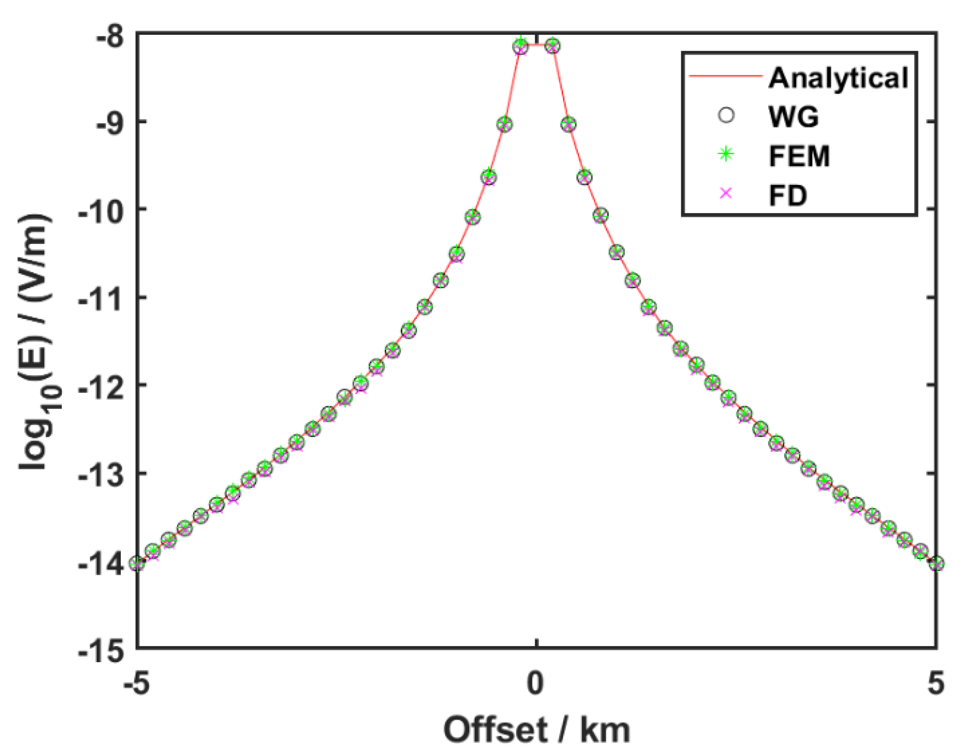
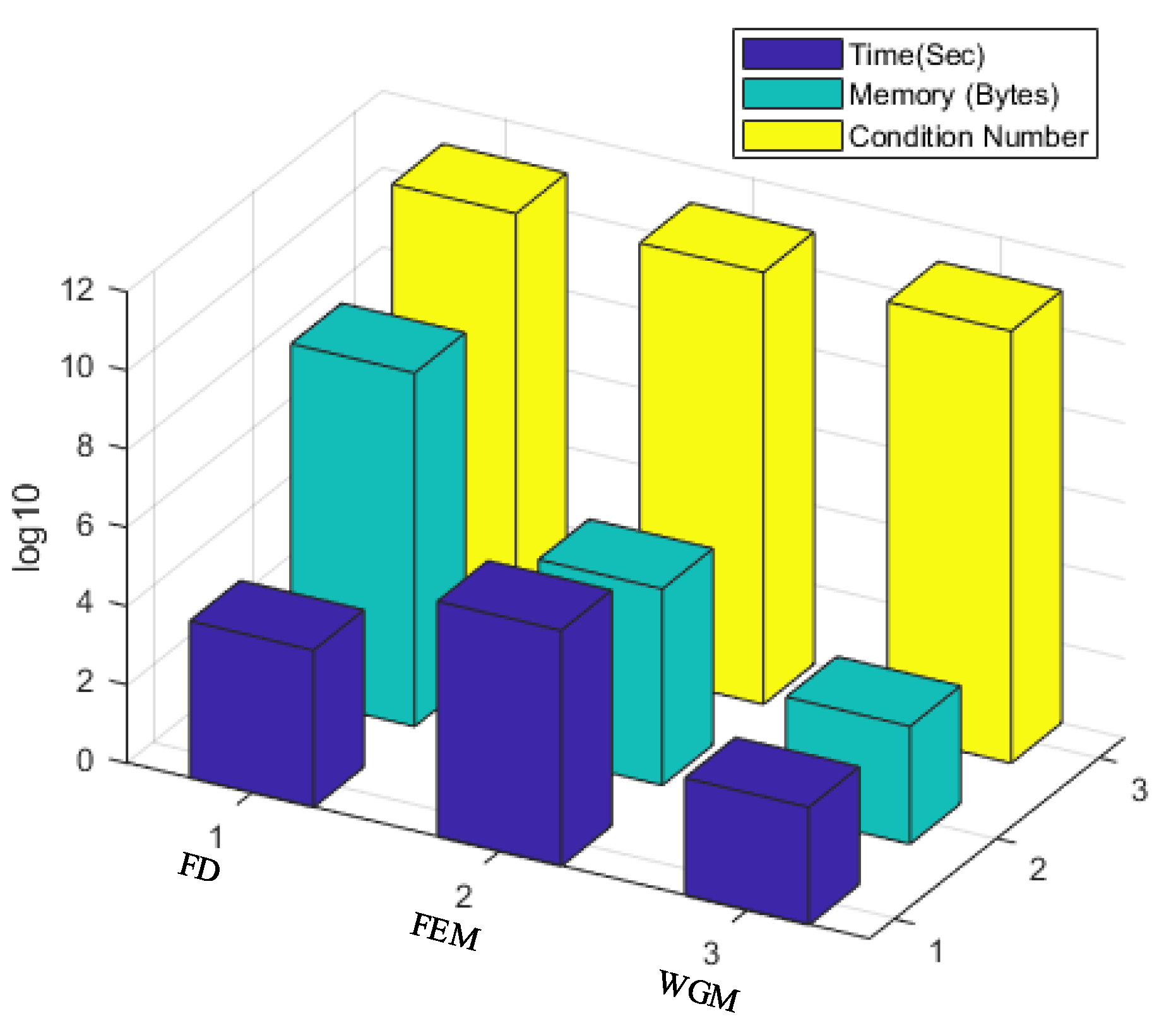
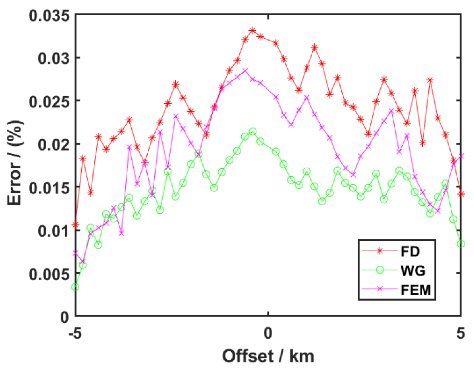
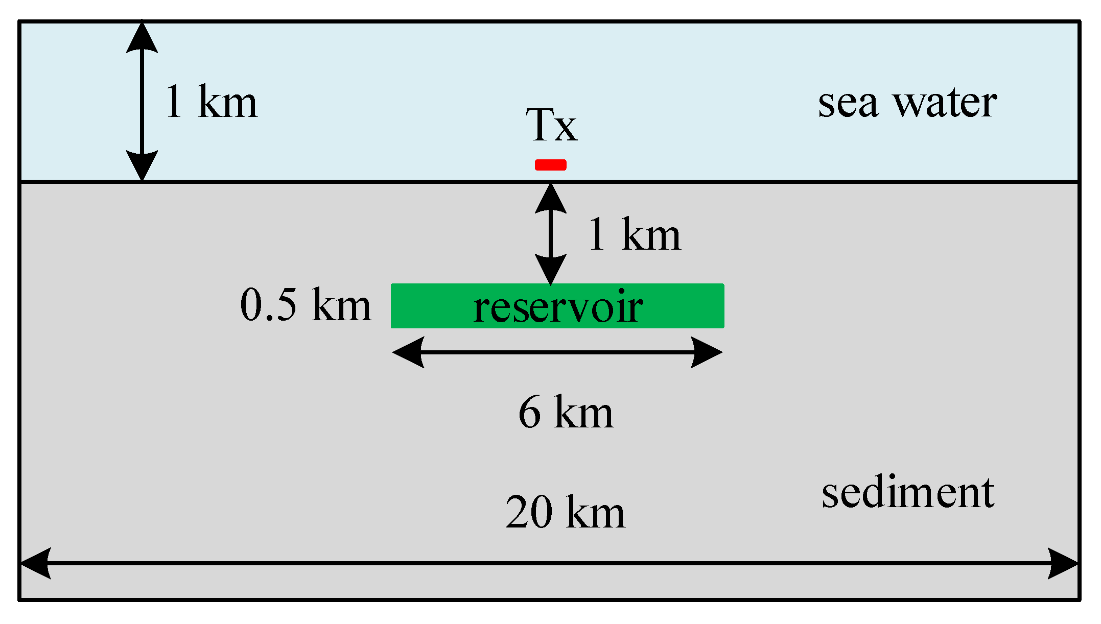
3.1. Simple Model for Verification Algorithm

To validate the proposed algorithm, we initially tested it on a simple 1D model with an isotropic medium, as shown in Figure 1; the layered geoelectrical model parameters are shown in

Table 1. Parameters of the horizontally layered geoelectrical model.

Parameters	Symbols	Magnitude
Frequency	f	0.5 Hz
Air	${\mathit{\sigma }}_{air}$	${10}^{-8}$ S/m
Seawater	${\mathit{\sigma }}_{sw}$	3.30 S/m
Sediment	${\mathit{\sigma }}_{sm}$	1.0 S/m
Hydrocarbon	${\mathit{\sigma }}_{hc}$	0.1 S/m

. An electric dipole in the horizontal direction was used to excite the electromagnetic field. The excitation source was along the y-axis, with the source coordinates of (0, 0, 950) m, located 50 m above the seafloor. The computation domain was discretized into a series of $2^{\left(\mathit{Nr}+ \mathit{Nc}\right)}$ elements, where $\mathit{Nr}=64$ and $\mathit{Nc}=256$. The Hankel transform method was used to calculate the analytical solution, which was compared with results from the WGM. Figure 2 shows the comparison of modeling results from the WGM, 1D analytical method, and other numerical methods. The meshes for the three numerical methods were the same. Figure 2 shows that the WGM results generally agree with the analytical solution, FEM, and FDM. The solution errors calculated by the WGM and other numerical methods (i.e., FEM and FDM) are shown in Figure 3. The maximum WGM error was 2.1%, whereas those for FEM and FDM were 2.7% and 3.3%, respectively, demonstrating that WGM provides a highly accurate solution. Figure 4 shows a comparison of the computational efficiency between WGM and other numerical methods. The required computational time and memory for WGM were lower than those for FDM and FEM, and the condition numbers of these three methods were almost the same. The calculation times for FEM and FDM were approximately 250 and 8 times that of WGM, respectively. These results demonstrate that the proposed approach may be used for efficient and accurate CSEM modeling.

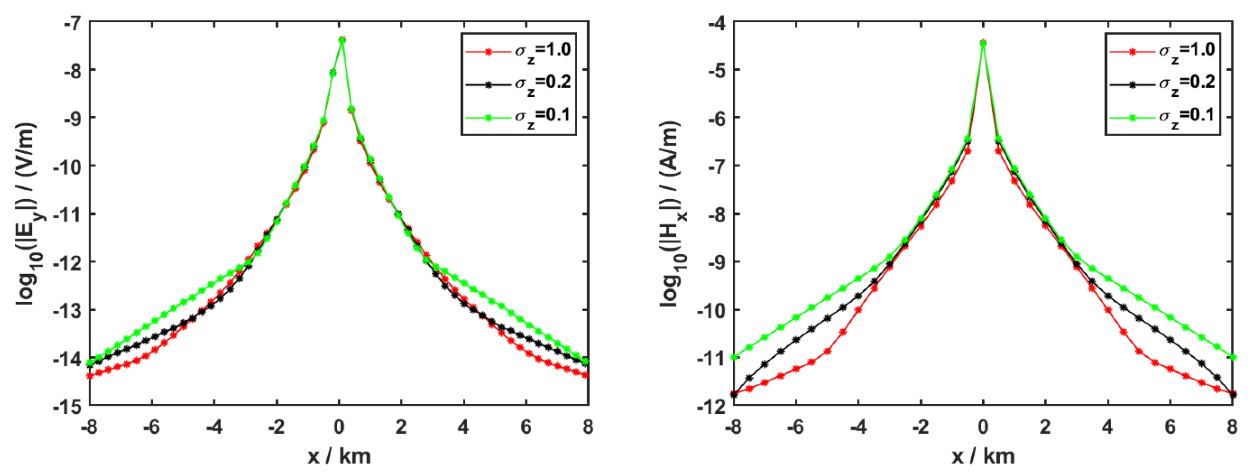
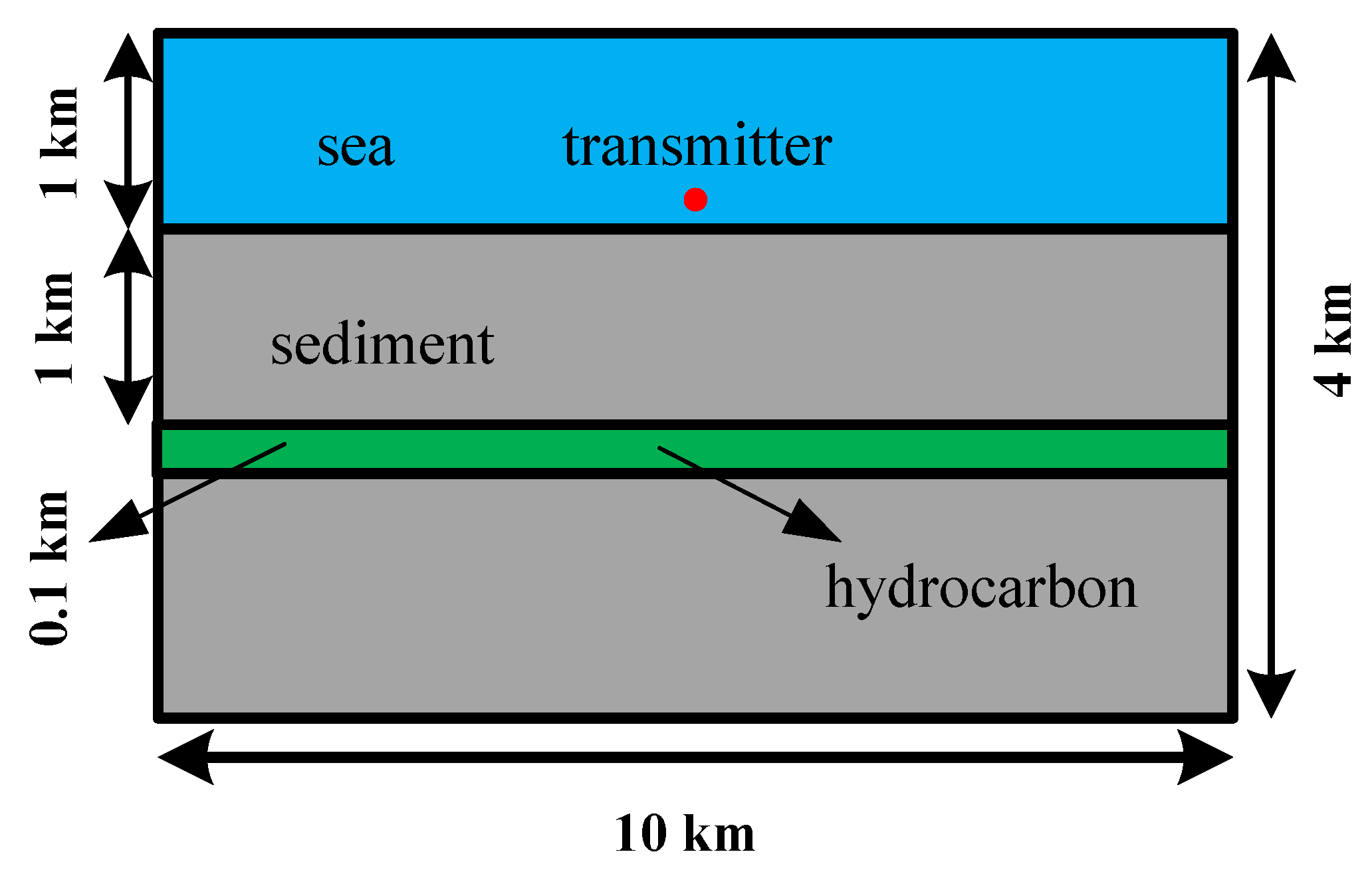
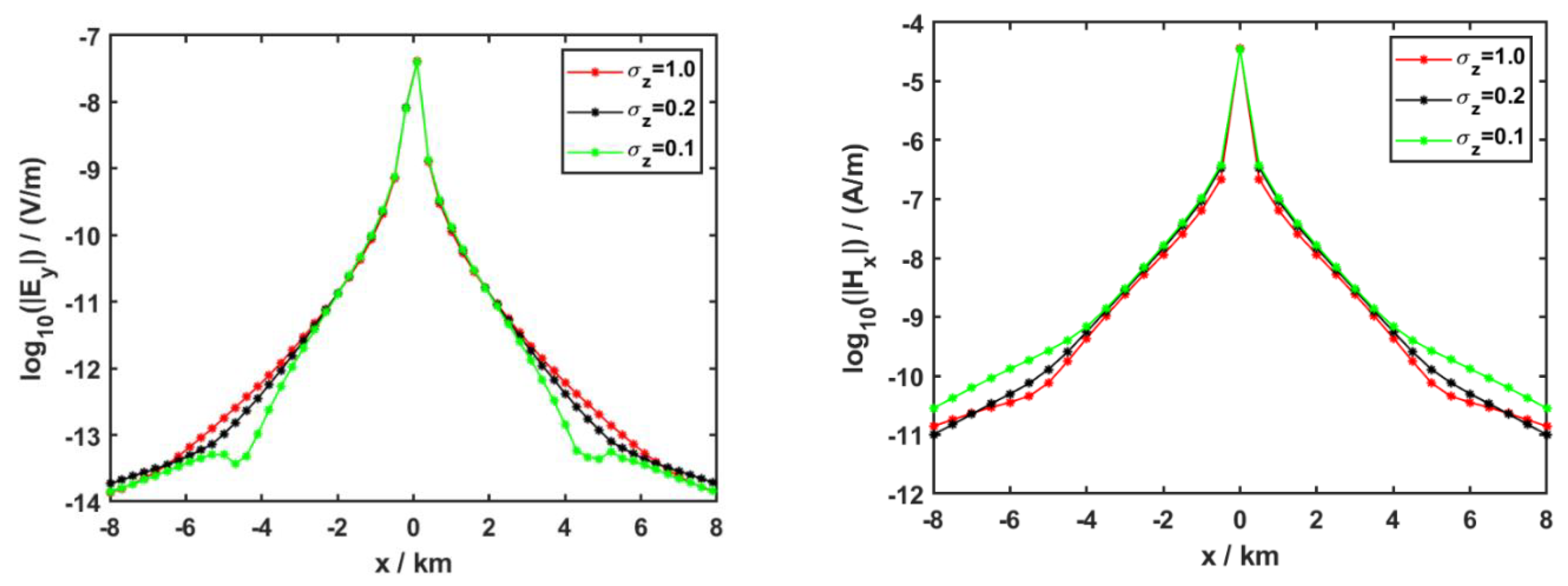
3.2. Anisotropy in the Sediment

We also considered a 2D model wherein the sedimentary layer was anisotropic and the reservoir was isotropic, as shown in Figure 5; the model parameters are listed in

Table 2. Parameters of the reservoir model.

Parameters	${\mathit{\sigma }}_{\mathit{x}}\left(\mathbf{S}/\mathbf{m}\right)$	${\mathit{\sigma }}_{\mathit{y}}\left(\mathbf{S}/\mathbf{m}\right)$	${\mathit{\sigma }}_{\mathit{z}}\left(\mathbf{S}/\mathbf{m}\right)$
Air	1 × 10−8	1 × 10−8	1 × 10−8
Seawater	3.3	3.3	3.3
Sediment	1.0	1.0	1.0, 0.2, 0.1
Reservoir	0.02	0.02	0.02

. An electric dipole source in the y-direction was used to excite the electromagnetic field. The excitation source was placed at (0, 0, 950) m and located 50 m above the seafloor, with excitation frequencies of 0.25, 0.5, and 1 Hz. The receiving stations were placed on the seafloor. The computational domain was discretized into a series of $2^{\left(\mathit{Nr}+ \mathit{Nc}\right)}$ elements, where $\mathit{Nr}=128$ and $\mathit{Nc}=256$. To examine the effects of conductivity on the MCSEM responses, we set the anisotropy coefficients of the background medium to 1, 5, and 10, which are consistent with the literature on conductivity anisotropy [22,23,24].

Figure 6, Figure 7 and Figure 8 depict the responses of the horizontal electric field, ${\mathrm{E}}_y$, and the horizontal magnetic field, Hx, under different vertical conductivity settings (${\mathit{\sigma }}_z$). Based on these figures, we found that ${\mathrm{E}}_y$ and Hx were affected by changes in vertical conductivity, which became more pronounced with a decrease in vertical conductivity. When the frequency was 0.25 Hz, the change in the ${\mathrm{H}}_x$ component was opposite to that in the ${\mathrm{E}}_y$ component. These results demonstrate that the anisotropic effect cannot be neglected.

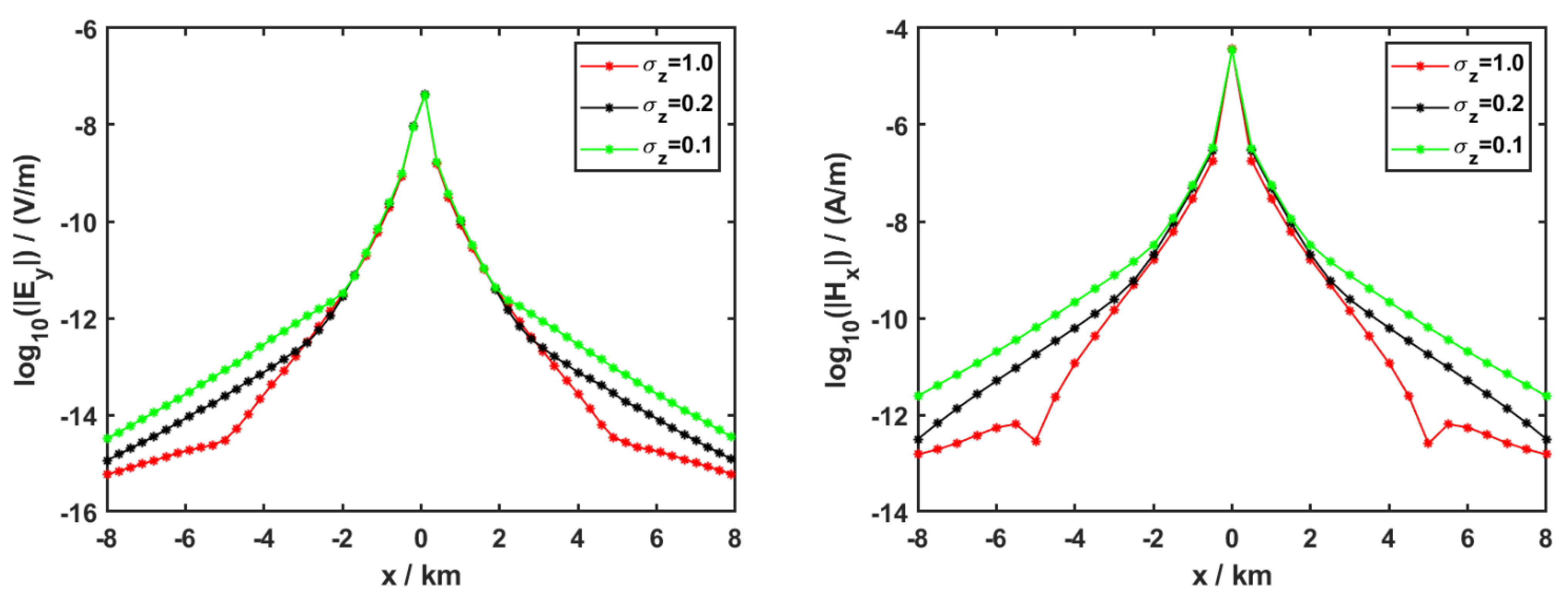
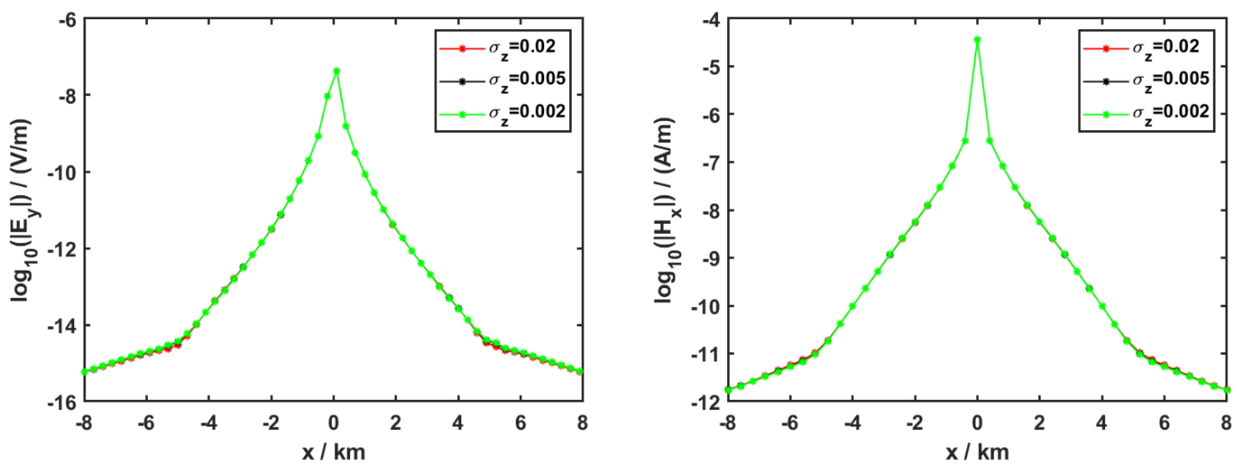
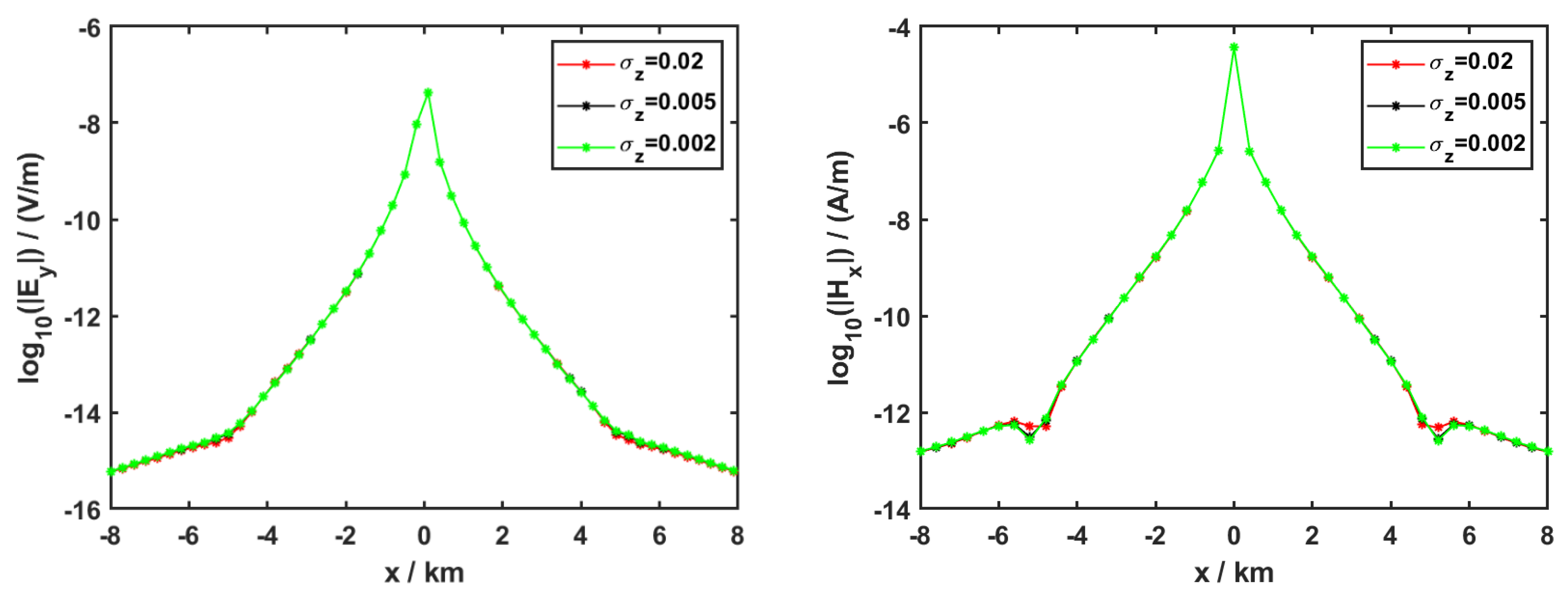
3.3. Anisotropy in the Reservoir

To investigate the effect of reservoir anisotropy, we considered a 2D model wherein the background medium was isotropic and incorporated an anisotropic reservoir; the background conductivity was 1 S/m. The geometric model parameters are presented in Figure 5. The horizontal conductivity of the reservoir was 1 S/m and remained constant, whereas the vertical conductivity of the reservoir varied from 0.02 to 0.002 S/m. The excitation frequencies were the same (0.25, 0.5, and 1 Hz). The computation domain was discretized into a series of $2^{\left(Nr+Nc\right)}$ elements, where $Nr=128$ and $Nc=256$. The receivers were located on the seafloor.

Figure 9, Figure 10 and Figure 11 depict the responses of the horizontal electric field, ${\mathrm{E}}_y,$ and magnetic field, ${\mathrm{H}}_x,$ along the seafloor for three different vertical conductivities ${\mathit{\sigma }}_z=\left(0.02, 0.005, 0.002\right) \mathrm{S}/\mathrm{m}$. These figures show that the electric field distributions in the three cases were very similar, indicating that the MCSEM responses were not strongly affected by the vertical conductivity of the anisotropic reservoir.

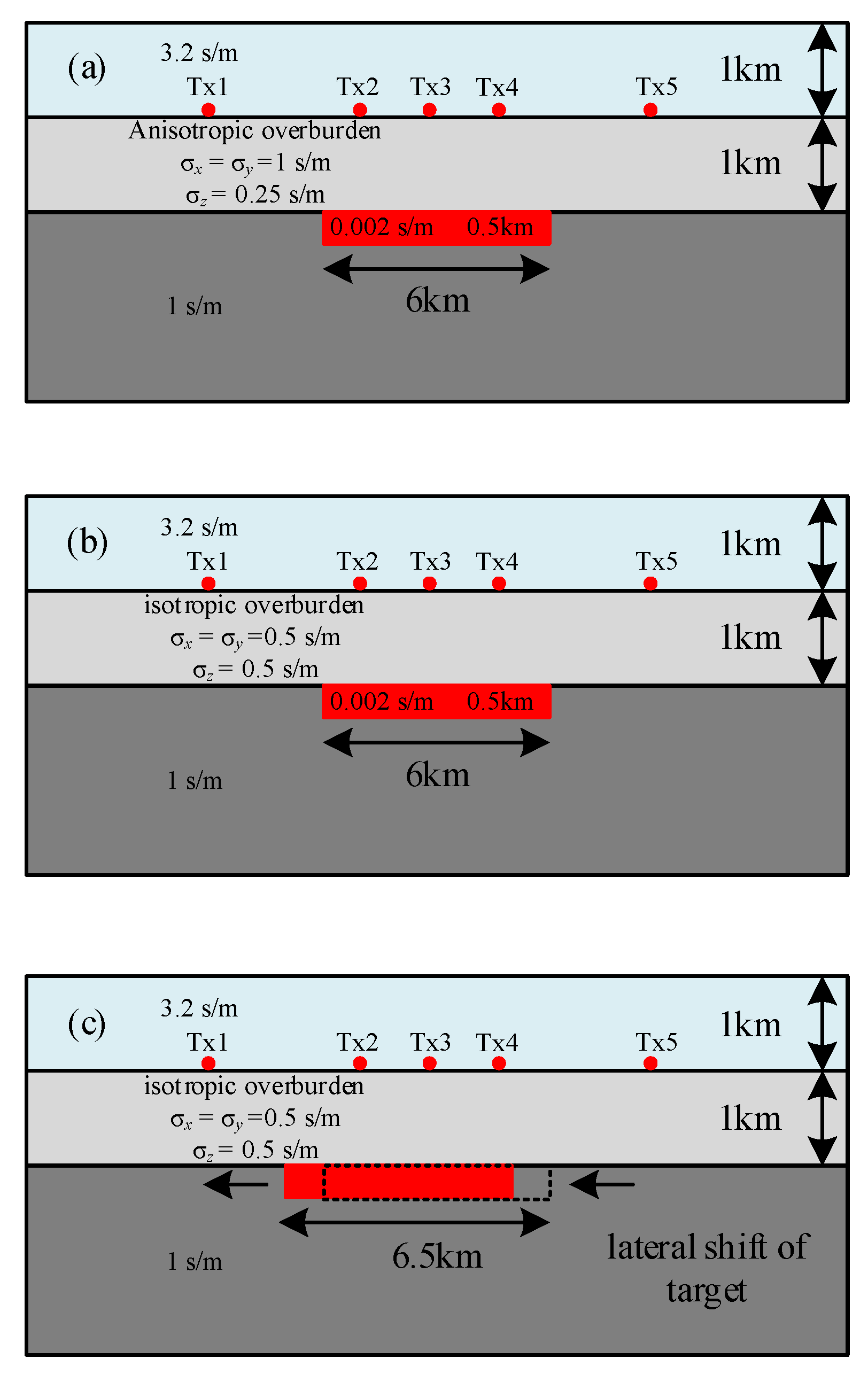
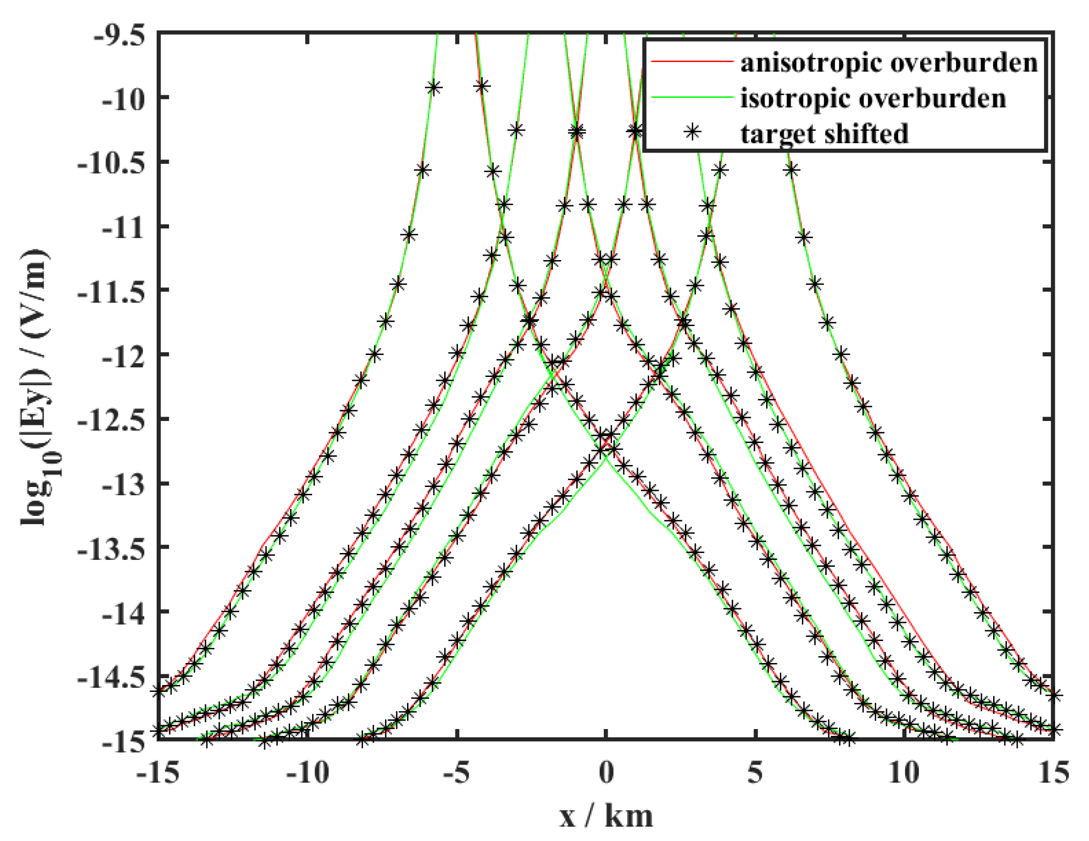
3.4. Effect of Isotropic and Anisotropic Overburdens on Underlying Targets

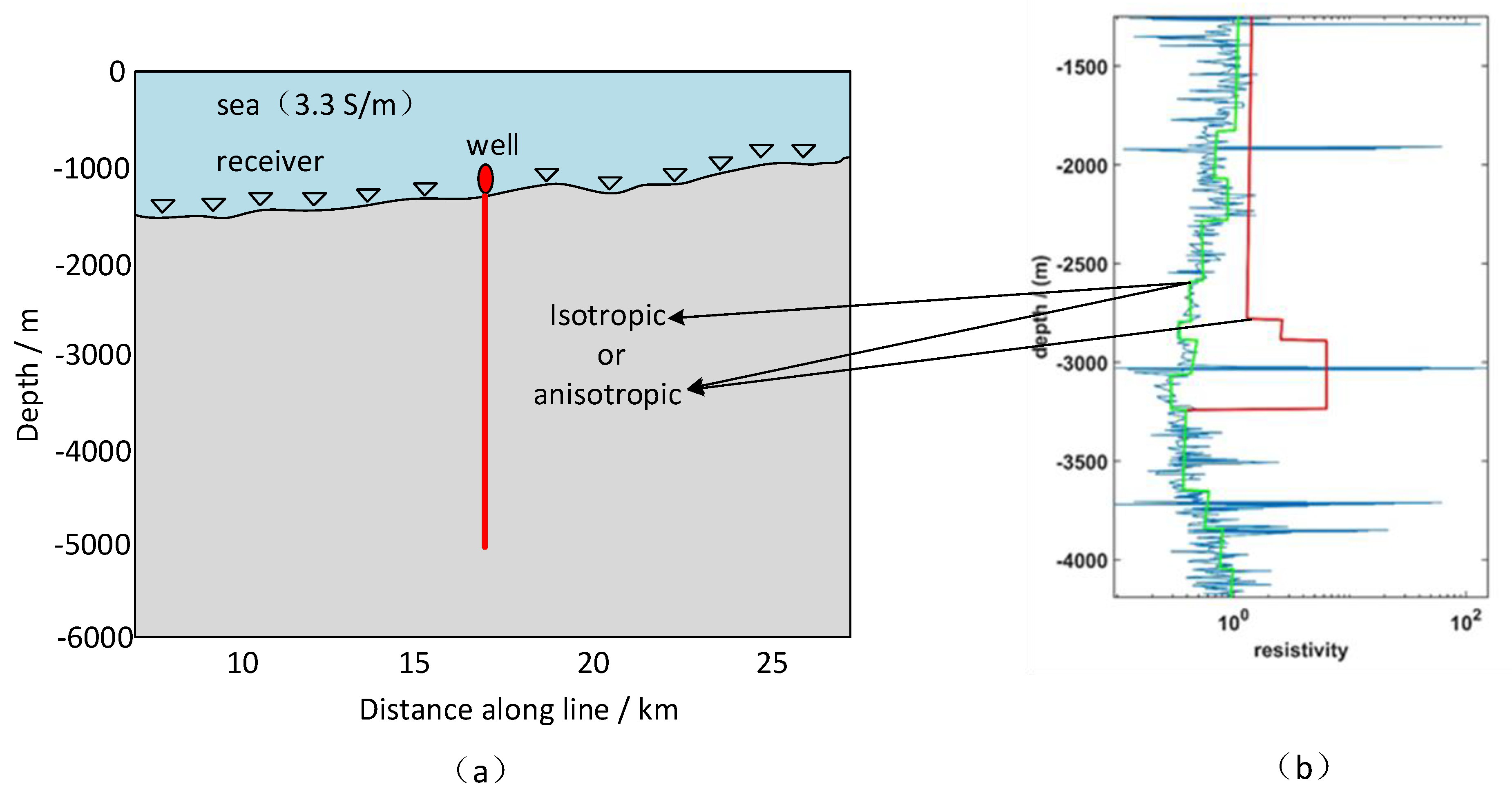
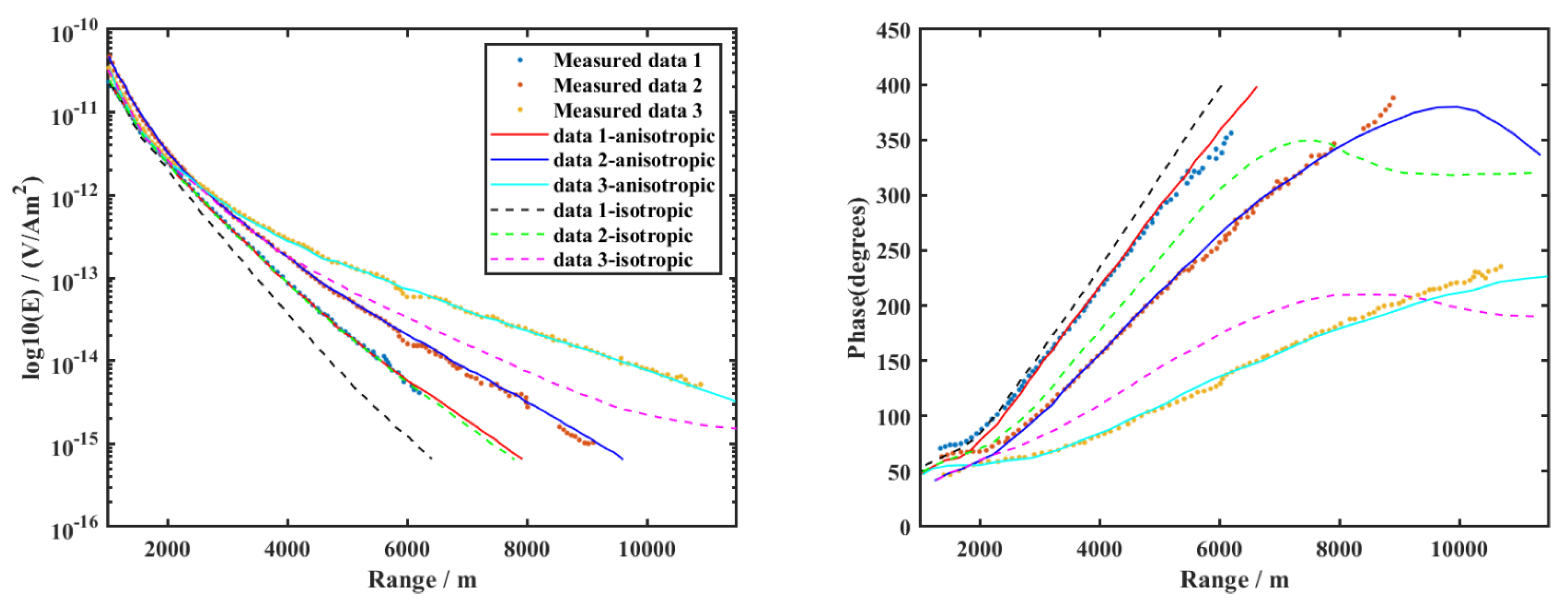
To investigate the effects of the different overburdens on CSEM responses, we considered three cases using a model with overburden and target body layers. In the first case, the overburden layer was anisotropic (Figure 12a), while it was isotropic in the second case (Figure 12b). The geometric structures of the first and second cases were the same, although the conductivity settings of the overburden layer differed. The third case was a variation of the second case with the target body position moved 0.5 km along the horizontal direction (Figure 12c). A series of horizontal electric dipole sources with a frequency of 0.25 Hz positioned in the y-direction were used to excite the electromagnetic field. There were five excitation sources from left to right: (−5000, 0, 950), (−2000, 0, 950), (0, 0, 950), (2000, 0, 950), and (5000, 0, 950) m, located 50 m above the seabed. In addition, receiving stations were placed on the seafloor at y = 0 m. The computation domain was discretized into a series of $2^{\left(\mathit{Nr}+ \mathit{Nc}\right)}$ elements, where $\mathit{Nr}=128$ and $\mathit{Nc}=256$.

Figure 13 shows the amplitude of the electric field component, ${\mathrm{E}}_y$, of the five excitation sources at an excitation frequency of 0.25 Hz. The green and red curves in Figure 13 show that the CSEM responses significantly differed under various overburden conditions. It shows that the effect of anisotropy in the overburden is obvious. The black dotted lines and red curves show that the model responses in Figure 12c were almost the same as those in the anisotropic overburden model shown in Figure 12a in the range of −5 km –5 km. Thus, it may be concluded that if the seabed medium is anisotropic and we continue to regard it as isotropic, incorrect information may be obtained, including an inaccurate location and range of the anomaly.

3.5. Real Data

A 2D model with undulating terrain was constructed to perform forward calculations based on the resistivity values obtained from a coastal oil well in West Africa, as shown in Figure 14. The measured electric amplitude and phase data were acquired by Dana Petroleum in 2005 [25] using source frequencies of 0.125, 0.375, and 0.625 Hz. The sediment medium was considered as anisotropic or isotropic. The results were compared with the measured amplitudes and phases of the electric field. Figure 14a presents an elevation diagram of the undulating terrain, and Figure 14b illustrates the resistivity values (blue line) at different logging depths and block average values. The block average values of the measured resistivity were assumed to be the horizontal component (green line) of resistivity; the vertical component (red line) of resistivity was designed in this study. The vertical resistivity components were 1–5 times the horizontal components. We discretized the entire computation domain into the same size as in the numerical model examples. Figure 15 shows the comparison of the forward calculation results with the amplitudes and phases of the measured electric fields in the two cases. The calculated isotropic overburden results assumed that the resistivity values of the underground media were equal to the block average values of measured resistivity. The calculated anisotropic overburden results were obtained using the horizontal and vertical resistivity components designed in this study, as shown in Figure 14b. Figure 15 shows that the CSEM responses, which were calculated by taking the block averages of the measured resistivities as the resistivities of the isotropic medium, greatly differed from the measured electric field amplitudes and phases. The anisotropic model results provide a much better match to the measured data. Therefore, the forward simulation of the simple 2D model based on logging resistivity data demonstrates the need for anisotropic inversion models to interpret data.

4. Conclusions

A WG algorithm was developed to solve the forward modeling problem of 2D MCSEM with conductivity anisotropy. We demonstrated that the proposed algorithm was reliable and efficient, regardless of whether an isotropic or anisotropic medium model was utilized. The calculation efficiencies and accuracies of FEM, FDM, and WGM were compared; WGM outperformed FEM and FDM under the same mesh conditions. The numerical results also indicated that the anisotropic characteristics influenced the electromagnetic field.

The effect of sediment anisotropy on the CSEM response was much greater than that of reservoir anisotropy. A simplified 2D model based on logging resistivity information and real elevation was established, and numerical simulation calculations were conducted for isotropic and anisotropic media. The results were compared with measured data, and the anisotropic model results were in better agreement with measured data than the isotropic model results; this highlights the need for anisotropic earth models for interpreting data and the need to perform anisotropic inversion. Future research will focus on solving 3D MCSEM forwarding and inversion problems using the WG algorithm.

References

1. Srnka, L.J.; Carazzone, J.J.; Ephron, M.S.; Eriksen, E.A. Remote reservoir resistivity mapping. Lead. Edge 2006, 25, 972–975. [Google Scholar] [CrossRef]
2. Constable, S.; Srnka, L.J. An introduction to marine controlled-source electromagnetic methods for hydrocarbon exploration. Geophysics 2007, 72, WA3–WA12. [Google Scholar] [CrossRef]
3. Li, Y.; Key, K. 2D marine controlled-source electromagnetic modeling, Part 1: An adaptive finite-element algorithm. Geophysics 2007, 72, WA51–WA62. [Google Scholar] [CrossRef] [Green Version]
4. Yuji, M. 2-D electromagnetic modeling by finite-element method with a dipole source and topography. Geophysics 2012, 65, 465–475. [Google Scholar]
5. Kerry, K. MARE2DEM: A 2-D inversion code for controlled-source electromagnetic and magneto telluric data. Geophys. J. Int. 2016, 207, 571–588. [Google Scholar]
6. Josef, P.; Tomáš, V. Finite-difference modelling of magnetotelluric fields in two-dimensional anisotropic media. Geophys. J. Int. 1997, 128, 505–521. [Google Scholar]
7. Arash, J.G.; Hiroshi, T. Efficient FDTD algorithm for plane-wave simulation for vertically heterogeneous attenuative media. Geophysics 2007, 72, H43–H53. [Google Scholar]
8. Aria, A.; Peter, M.V.D.; Tarek, M.H. An integral equation approach for 2.5-dimensional forward and inverse electromagnetic scattering. Geophys. J. Int. 2006, 165, 744–762. [Google Scholar]
9. Daubechies, I. Orthonormal bases of compactly supported wavelet. Commun. Pure Appl. Math. 1988, 41, 906–996. [Google Scholar] [CrossRef] [Green Version]
10. Moller, N.O. Wavelets in Scientific Computing. Ph.D. Thesis, Technical University of Denmark, Lyngby, Denmark, 1998. [Google Scholar]
11. Hussaina, N.; Karsitia, M.N.; Yahyaa, N.; Jeotia, V.; Yahyab, N. 2D wavelets Galerkin method for the computation of EM field on seafloor excited by a point source. Int. J. Appl. Electromagn. Mech. 2017, 53, 631–644. [Google Scholar] [CrossRef]
12. Chen, H.B.; Li, T.L. 3D Marine Controlled-Source electromagnetic modeling in an Anisotropic Medium Using a Wavelet-Galerkin Method with a Secondary Potential Formulation. Geophys. J. Int. 2019, 219, 373–393. [Google Scholar] [CrossRef]
13. Ramananjaona, C.; MacGregor, L.; Andréis, D. Sensitivity and inversion of marine electromagnetic data in a vertically anisotropic stratified earth. Geophys. Prospect. 2011, 110, 341–360. [Google Scholar] [CrossRef]
14. Brown, V.; Hoversten, M.; Key, K.; Chen, J. Resolution of reservoir scale electrical anisotropy from marine CSEM data. Geophysics 2012, 77, E147–E158. [Google Scholar] [CrossRef]
15. Newman, G.A.; Commer, M.; Carazzone, J.J. Imaging CSEM data in the presence of electrical anisotropy. Geophysics 2010, 75, F51–F61. [Google Scholar] [CrossRef]
16. Kong, F.N.; Johnstad, S.E.; Rosten, T.; Westerdahl, H. A 2.5D finite-element modeling difference method for marine CSEM modeling in stratified anisotropic media. Geophysics 2008, 73, F9–F19. [Google Scholar] [CrossRef]
17. Weiss, C.J.; Newman, G.A. Electromagnetic induction in a fully 3D anisotropic earth. Geophysics 2002, 67, 104–114. [Google Scholar] [CrossRef]
18. Freund, R.W.; Nachtigal, N.M. QMR: A quasi-minimal residual method for non-Hermitian linear systems. Numer. Math. 1991, 60, 315–339. [Google Scholar] [CrossRef] [Green Version]
19. Debnath, L.; Shah, F.A. Multiresolution Analysis and Construction of Wavelets. In Wavelet Transforms and Their Applications; Birkhäuser: Boston, MA, USA, 2015; Volume 45, pp. 375–440. [Google Scholar]
20. Li, B.; Chen, X. Wavelet-based numerical analysis: A review and classification. Finite Elem. Anal. Des. 2014, 81, 14–31. [Google Scholar] [CrossRef]
21. Latto, A. The Evaluation of Connection Coefficients of Compactly Supported Wavelets; Princeton: New York, NY, USA, 1991. [Google Scholar]
22. Keller, G.V.; Frischknecht, F.C. Electrical Methods in Geophysical Prospecting; Pergamon Press: Oxford, UK, 1966. [Google Scholar]
23. Christensen, N.B. Difficulties in determining electrical anisotropy in subsurface investigations. Geophys. Prospect. 2000, 48, 1–19. [Google Scholar] [CrossRef]
24. Aissaoui, R.; Bounif, A.; Zeyen, H.; Messaoudi, S.A. Evaluation of resistivity anisotropy parameters in the Eastern Mitidja basin, Algeria, using azimuthal electrical resistivity tomography. Near Surf. Geophys. 2019, 17, 359–378. [Google Scholar] [CrossRef]
25. Ramananjaona, C.; Macgregor, L. 2.5D inversion of CSEM data in a vertically anisotropic earth. J. Phys. Conf. Ser. 2010, 255, 012004. [Google Scholar] [CrossRef]
Figure 1. Schematic of horizontally layered geoelectrical model.
Minerals 12 00124 g001
Figure 2. Comparison of the electrical field of different numerical methods and the 1D analytical solution.
Minerals 12 00124 g002
Figure 3. Errors associated with the different numerical methods among 1D analytical solutions.
Minerals 12 00124 g003
Figure 4. Comparison of computational efficiency among different numerical methods (z-axis is logarithmic coordinate).
Minerals 12 00124 g004
Figure 5. Schematic of anisotropic sediment with a hydrocarbon reservoir model.
Minerals 12 00124 g005
Figure 6. Responses of E y and H x computed using the WGM at f = 0.25 Hz.
Minerals 12 00124 g006
Figure 7. Responses of E y and H x computed using the WGM at f = 0.5 Hz.
Minerals 12 00124 g007
Figure 8. Responses of E y  and H x  computed using the WGM at f = 1.0 Hz.
Minerals 12 00124 g008
Figure 9. Responses of E y and H x computed using the WGM at f = 0.25 Hz.
Minerals 12 00124 g009
Figure 10. Responses of E y and H x computed using the WGM at f = 0.5 Hz.
Minerals 12 00124 g010
Figure 11. Responses of E y and H x computed using the WGM at f = 1.0 Hz.
Minerals 12 00124 g011
Figure 12. Typical 2D geoelectric model: (a) anisotropic overburden; (b) isotropic overburden; (c) changes to the target body position. The target moved 0.5 km to the left. The red dots represent the positions of the sources.
Minerals 12 00124 g012
Figure 13. Amplitudes of the electric fields, E y , for five excitation sources.
Minerals 12 00124 g013
Figure 14. (a) Geometric diagram of simplified 2D model established according to real elevation and (b) the resistivity log from a well. The blue line is the real measured resistivity. The green line is the block average of measured resistivity, which is considered to be a horizontal component of resistivity. The red line is the vertical component of resistivity that is 1–5 times the horizontal component of resistivity.
Minerals 12 00124 g014
Figure 15. Comparisons of electric field amplitude and phase data for models with different resistivity settings using measured data. The degree of fit between the results of the anisotropic model and measured data was higher than that for the isotropic model.
Minerals 12 00124 g015