A Method for Assessing the Thickness of Cobalt-Rich Crust on Seamounts and Its Application on the Il’ichev Guyot

Abstract

Seamount cobalt-rich crusts are rich in cobalt resources and are sought after worldwide. Among different affecting parameters, crust thickness is the most important in evaluating cobalt-rich crust resources in seamounts. Generally, there are two challenges to crust thickness evaluation: firstly, due to high operating costs, most geological stations for seamount exploration have sparse sampling distributions so there are insufficient data to estimate the crust thickness distribution; secondly, a single evaluation method has advantages and disadvantages, and it is not feasible to benefit from the advantages only. These methods cannot simultaneously make full use of the sampling data in local areas, providing a more appropriate evaluation of the whole area. As a result, the estimated results cannot fully reflect the thickness distribution. Based on the thickness data of the station survey and topographic data, geostatistical units are divided, and a comprehensive crust thickness assessment scheme is established on the ArcGIS platform. To this end, the adjacent area method is applied to calculate the crust thickness within the influence range of the station. Combined with the station buffer radius and Thiessen polygon method, the crust thickness within 1.5 km of the survey station was estimated. Then the “slope–distance” Kriging interpolation method was used to calculate the crust thickness in the study area, and the crust thickness in the optimal effective radius area was given to compensate for the missing part in the first step. Finally, the geological blocks were divided using the topographic classification method, and the crust thickness of the remaining unassigned regions was estimated using the mathematical expectation method. The proposed method was applied to evaluate the Il’ichev Guyot’s crust thickness and reasonable results were achieved. It was found that the thickness estimation of the area near the station is consistent with the measured values. Since finer topographic data are used in the calculation, the thickness estimation result is more detailed. In this regard, a simple and effective calculation method was established on the ArcMap platform. The mathematical expectation estimation method of the crust thickness, based on the topographic and geomorphological classification from the perspective of the mineralization mechanism, compensates for the drawbacks of the first two methods originating from the lack of data points. The results show that the proposed method is an appropriate scheme to evaluate seamount crust thickness without comprehensive investigation.

1. Introduction

Seamount cobalt-rich crust are rich mineral resources, which have attracted scholars in the past two decades. Considering their high economic value, it is of great significance to survey and analyze the spatial distribution of cobalt-rich crust resources [1].

The crust thickness, wet density, water content, coverage rate, and metal concentration, which reflect the quality, grade, and reserves of mineral resources, are collectively referred to as the parameters of cobalt-rich crust resources. Among these indicators, crust thickness is an important parameter in the evaluation [2].

The understanding and analysis of the mineralization pattern of cobalt-rich crusts and the influencing factors are undeniable prerequisites for resource assessment. In this regard, numerous investigations have been carried out to analyze the relationship between crust mineralization and the bedrock type [3,4,5,6,7,8,9,10,11,12,13,14,15]. The bedrock of the crust consists of basalt, pyroclastic rock, phosphate rock, siliceous rock, or limestone [3,4]. Generally, the crust thickness of basalt, volcanic rock, and phosphate rock is larger than that of siliceous rock, and the formation of the crust is closely related to water depth [5]. Among these materials, the highest average thickness of crusts occurs in pyroclastic and basalt rocks, while loose and brittle rocks such as tuff and phosphate rocks have a thin crust on the surface. It is worth noting that siliceous rocks are not conducive to the growth of the crust [5]. The crust-forming materials mainly originate from seawater and are very little affected by bedrock [5,6]. Investigations have been carried out on the relationship between water depth and the cobalt-rich crust thickness, indicating that the crust growth is closely related to the water depth of the seamount. Globally, crusts grow in water depths ranging from 400 to 4000 m, mainly restricted by the low oxygen concentration zone (OMZ) and carbonate compensation depth (CCD). Under these conditions, crusts grow while there are seamount slopes in between [6,7,8]. Studies show that different water depths affect the growth of the crust; generally, 80% of about 41 mm thick crusts grow at a water depth of 1000–3000 m, of which 55% is at a water depth of 1500–2500 m [9]. Similarly, crusts of various thicknesses form at a depth of 2800 m, and half of them are larger than 50 mm, among which crusts larger than 100 mm mainly grow on the Pacific seamount at a depth of 2500 m [11,12,13,14].

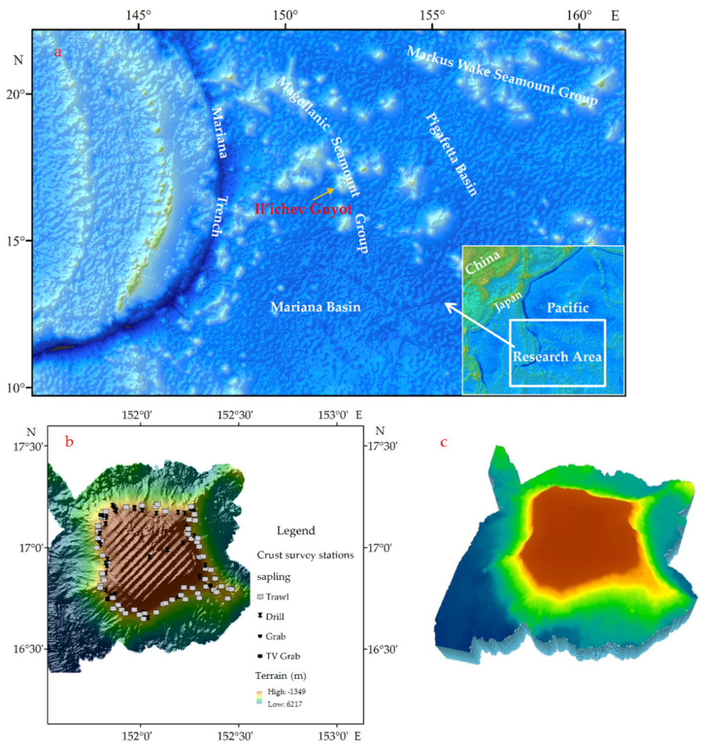
The Magellanic Sea Mountain chain is a large-scale submarine volcanic chain within the Kula plate. Figure 1 shows that this chain is located between the Mariana Trench to the west, the Pigafetta Basin to the northeast, and the Mariana Basin to the southwest. The seamount chain consists of more than ten seamounts and stretches more than 1000 km in the northwest direction [10,12]. The Il’ichev seamount, located in the Magellan seamount chain in the western Pacific Ocean, is a flat-topped seamount with a roughly square distribution, as shown in Figure 1. Since the compilation of the “95 Plan” in China, many of these seamounts have been explored. Based on the performed surveys, the Magellan Seamount chain is a volcanic uplift formed on the top of the bedrock of the Mid-Jurassic–Cretaceous ocean floor where basalt is the most abundant rock in the seamount. The main sedimentary face of the seamount consists of volcanic clastic rocks, carbonate rocks, and clay. Since the formation of the volcanic plateau in the Early Cretaceous, an atoll development phase has passed. Due to the volcanic/regional tectonic effect, three to four up-and-down rotational changes appeared in the Middle and Late Albian period. This phenomenon had an undeniable impact on crustal mineralization.

Currently, different techniques are applied to evaluate the crust thickness. These techniques can be mainly divided into the following three categories: (i) The average crust thickness is mostly used for estimation [16]. When there is no grid to determine the stations, the thickness of the adjacent area can be estimated based on the crust thickness of adjacent stations [17]. (ii) The crust thickness can also be estimated by spatial interpolation. In this method, the crust thickness is estimated according to the topography slope and the distance between stations. The distance–slope Kriging interpolation method [1] falls in this category. (iii) Crust thickness can be estimated according to the restriction mechanisms of crust deposition and mineralization or topographic characteristics [18]. The fractal method [19,20] is an appropriate sample of this method.

Studies show that single evaluation methods have some advantages and disadvantages, and one cannot only benefit from the advantages. In these methods, the results do not reflect the thickness distribution, thereby leading to uncertainty in regional resource assessment. For example, (1) although the most accurate thickness data can be obtained according to the station survey, data are sparse so it is a challenge to comprehensively estimate the thickness of the whole area. (2) In Kriging, fractal, and block interpolation methods, the crust thickness is estimated according to spatial distributions such as station and topography, thereby covering a wide prediction range. However, the estimation accuracy is low when there are no or insufficient stations. That is, the reliability of the model prediction results is relatively low when the estimated area is far from known stations. (3) Based on the metallogenic restriction mechanism of crust deposition and the metallogenic theory [18], the regional crust thickness can be estimated statistically based on topographic characteristics. This technique is suitable for large surveying areas, especially multiple seamounts. However, this method does not reflect the local specificity.

In the present study, we employ the ArcGIS 10.0 (Esri) as technical environment to study the integrated thickness assessment method of the adjacent area method, the “slope–distance” Kriging interpolation method, and the terrain classification crust thickness mathematical expectation method to calculate the crust thickness based on the site survey thickness and topographic data. The main objective of this article is to obtain the spatial distribution of cobalt-rich crust resources in the seamounts. In this regard, the Il’ichev seamount in the Magellan seamounts is taken as an example to develop a comprehensive crust-thickness assessment scheme, calculate the thickness distribution, and compare and verify the performance of different methods. The achievements of this study are expected to be useful in other seamount crust-resource assessments.

2. Data

2.1. Data Sources

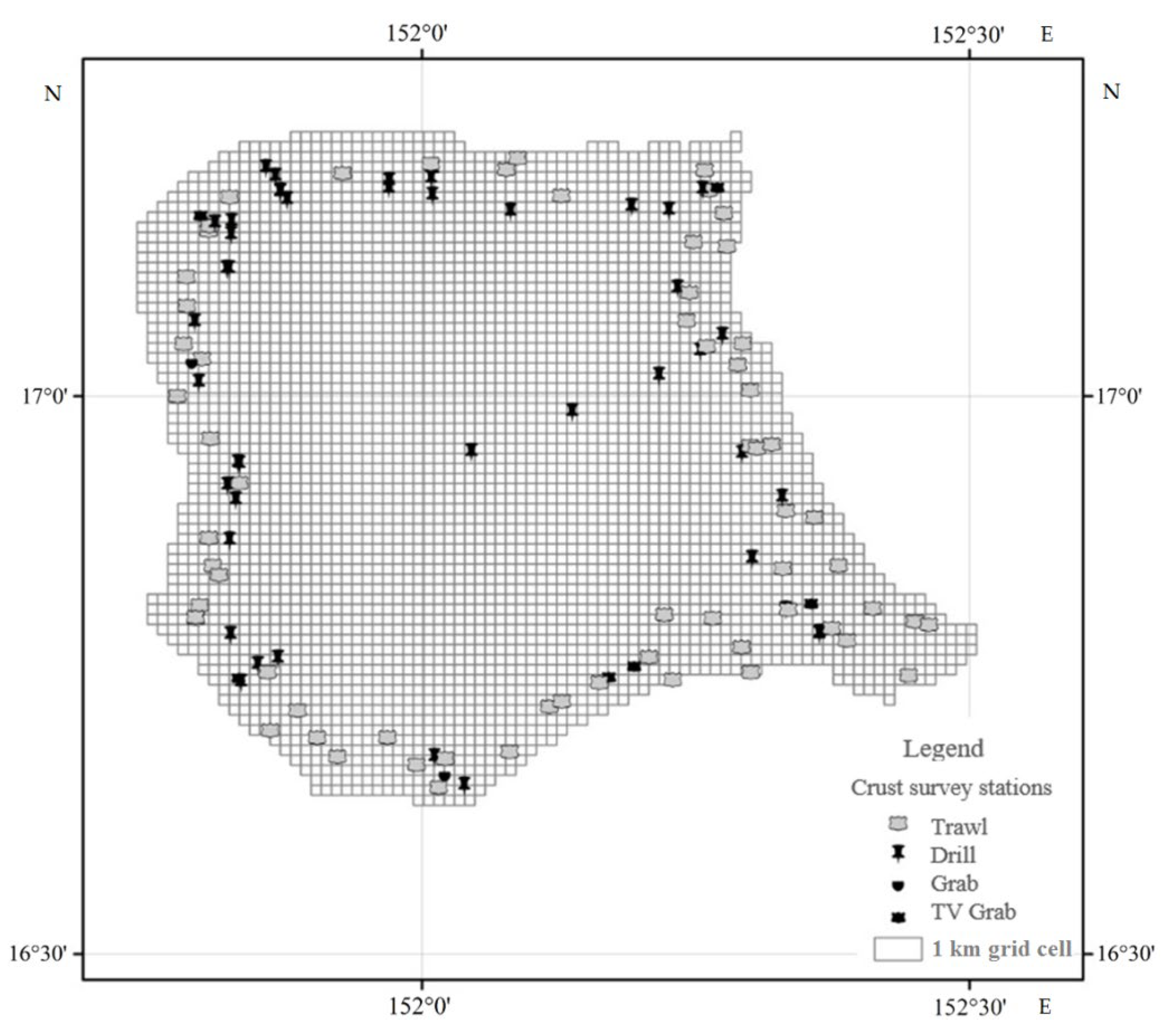
The Il’ichev seamount is one of the earliest seamounts for cobalt-rich crust prospecting in China. Since the 1990s, eight crusted surveys have been carried out, including DY95-9, DY95-10, DY105-11, DY105-15, DY105-16A, DY105-17B, DY 115-18, and DY 115-19. There are 109 crust survey stations, including 59 stations for geological trawl surveys, 40 stations for deep-sea shallow drilling surveys, and 10 stations for other sampling methods. In addition to geological sampling surveys, topographic and visual explorations have also been carried out.

2.2. Data Analysis

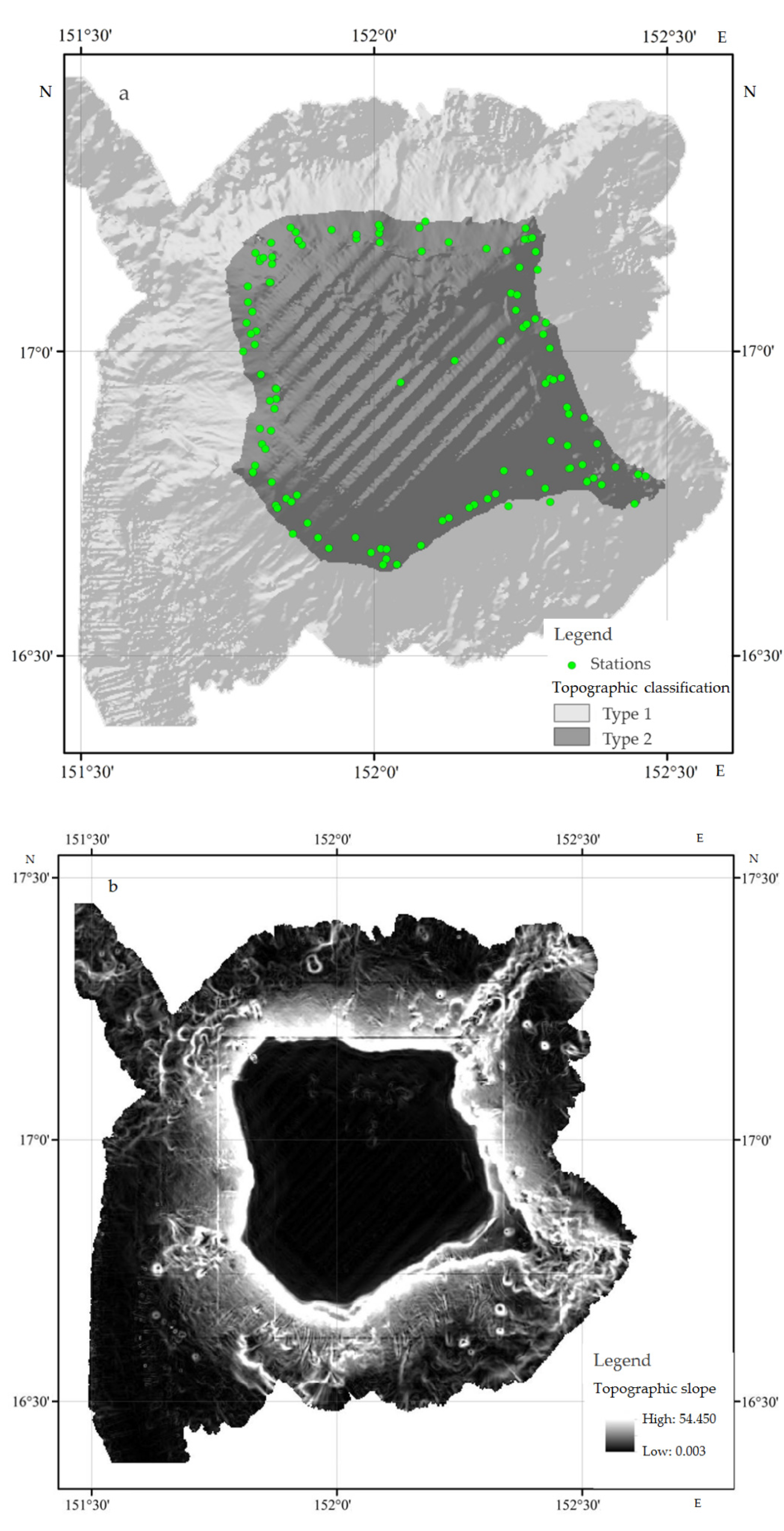
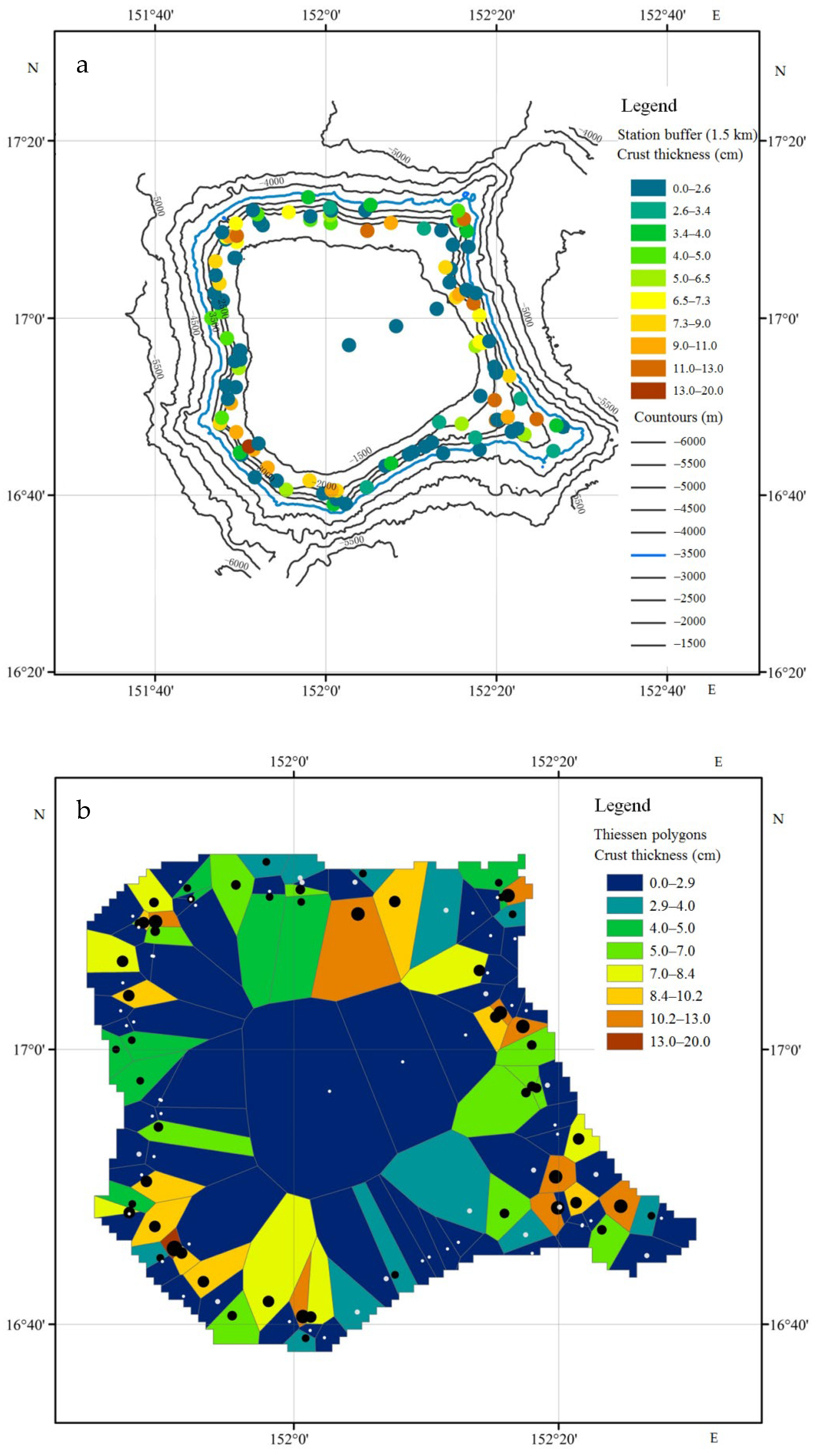
The geological sampling locations of the Il’ichev seamount crusts are around the edge and ridge of the seamount peak. Figure 2 shows that the distance between the stations is uneven, ranging from 1–2 km to 10 km. In order to estimate the crust thickness, it is necessary to determine the station coordinates and the unique crust thickness of the shallow drill and TV grab samples. Considering the long towing distance and large number of samples, the geographic coordinates of the trawling station were taken as the middle position between the starting and leaving points of the equipment. Then the crust thickness can be obtained as the median thickness of the samples. Although this technique is relatively accurate, its spatial distribution density is low and far from the requirements of calculating the distribution of crust resources.

The topographic data can be obtained through a shipborne multi-beam survey. The accuracy of topographic post-processing data is 230 m, which is much higher than that of the geological sampling survey.

The growth pattern and thickness of cobalt-rich crusts depend on topography [18]. The majority of landforms and micro-landforms are closely related to crust distribution. A micro-landform, which refers to relatively small-scale geomorphic forms, is the smallest geomorphic form unit and is a sub-landform that was developed on a small landform unit. Micro-landforms depend on the topography slope. The calculated topography slope of the seamount in Figure 2 reflects the rope-like accumulation at the ridge, indicating that the stations with good crust-like growth fall on the gentle and stable micro-landform in the area with a large relative slope change.

The growth of the cobalt-rich crust is restricted by the physical and chemical properties of seawater. When the water depth at the top edge of the seamount exceeds the water depth corresponding to the minimum oxygen content, its isobath can be regarded as the upper boundary of the ore body; otherwise, the isobath of minimum oxygen content is regarded as the upper boundary of the ore body. Based on this criterion, the upper boundary of the ore body is in the Il’ichev seamount’s top edge of the control range of the crust-sampling station, while the lower boundary can be a carbonate-compensated interface isobath. The depth of the carbonate compensation interface at the seamount is 3500 m. The lower boundary of the ore body can also be divided by topographic classification. Then, the ArcMap 10.0 unsupervised classification model can be applied to analyze the topographic data. In this method, the results of the seamount terrain are divided into two categories, and the boundary line of the classification result is 3500 m isobath. Therefore, the lower boundary of the crust thickness estimation is set to 3500 m, which is consistent with the depth of the carbonate compensation interface at the seamount.

The geological station buffer is calculated using ArcGIS 10.0, and the station is used to evaluate the crust thickness. The influence area of the geological station is estimated using the Thiessen polygon method. Meanwhile, the geological grid units were divided, the topography slope and station distance were calculated, and the “distance–slope” method was used to evaluate the crust thickness. The landform types can be classified according to landform data and calculated average crust thickness.

3. Methods

3.1. Division of Geostatistical Units

A statistical unit refers to a subspace domain of the evaluation area of cobalt-rich crust. It is worth noting that a cobalt-rich crust evaluation area contains several statistical units, which are much smaller than the entire evaluation area. Assume that A, a, and n are the evaluation area of cobalt-rich crust, the statistical unit, and the number of units, respectively. The following statistical relationship holds between these parameters: A = {a_i}, i = 1, 2,…, n.

The statistical unit is the smallest unit of statistical evaluation, which contains data related to geological characteristics, mineral parameters, and resource quantity. It is assumed that, within a unit, geological characteristics and mineral parameters are uniform. The units are considered to be differentiated so there is a spatial anisotropy of geological features and resource parameters between the units.

The division of statistical units is a fundamental process in the evaluation of mineral resources. Subsequently, the results of mineral resources can be expressed according to units. Whether the unit division is reasonable or not directly affects the evaluation results of mineral resources. Currently, the division method of geological units [21] and grid units [22] are widely used in this regard.

The main objective of the former method is to delineate statistical units at all levels by applying geological conditions and prospecting marks, which have a definite control effect on certain mineral resources [23]. This method has two key characteristics, namely clear ore control characteristics, and having different ore control conditions and prospecting marks under different scales. For example, if the central and western Pacific Ocean is taken as the evaluation area for cobalt-rich crust resources, the geomorphology of seamounts can be used as an indicator to classify the geological units. In this case, seamounts within the central and western Pacific Ocean are geological units. When a seamount is considered as the resource evaluation area, geological units are divided according to geological conditions, such as slope and water depth, that affect the growth of the cobalt-rich crust. This, in essence, is to divide the adjacent seamount slope block with similar ore control conditions into a single geological unit. At a similar water depth and seamount slope, the area adjacent to each geological station can be divided into different geological units. In conclusion, the cobalt-rich crust resources at different scales can be evaluated according to different geological units and geological indicators.

Grid unit division refers to dividing the evaluation area into several units by a regular grid, while the grid is used as the statistical unit. Grid units fit spatial data analysis techniques such as spatial interpolation of various mineral parameters and spatial extraction of geological features [23].

The partitioning methods of these three scales can be used simultaneously in a resource evaluation work of the same scale. For example, these methods can be used on large scales. The topographic and geomorphic classification method and the survey station adjacent area method can be applied to evaluate the seamount scale resource.

The working area of seabed solid mineral resource evaluation, including the survey area, exploration area, and resource area, collectively covers a large area, which is usually referred to as the seabed evaluation area. Smaller areas such as a seamount cover thousands of square kilometers [24], while larger areas such as the Pacific CC area of polymetallic nodules cover millions of square kilometers. The seabed evaluation area is equivalent to at least a dozen land geological maps at a scale of 1:100,000. The first process in large-scale (1:10,000, 1:50,000, 1:100,000) mineral resources evaluation maps is to divide statistical units. This process is especially important in seabed evaluation. The geostatistical unit division of cobalt-rich crust resources can be divided into the following three methods:

3.1.1. Topographic and Geomorphic Classification (Also Called the Geological Block Method)

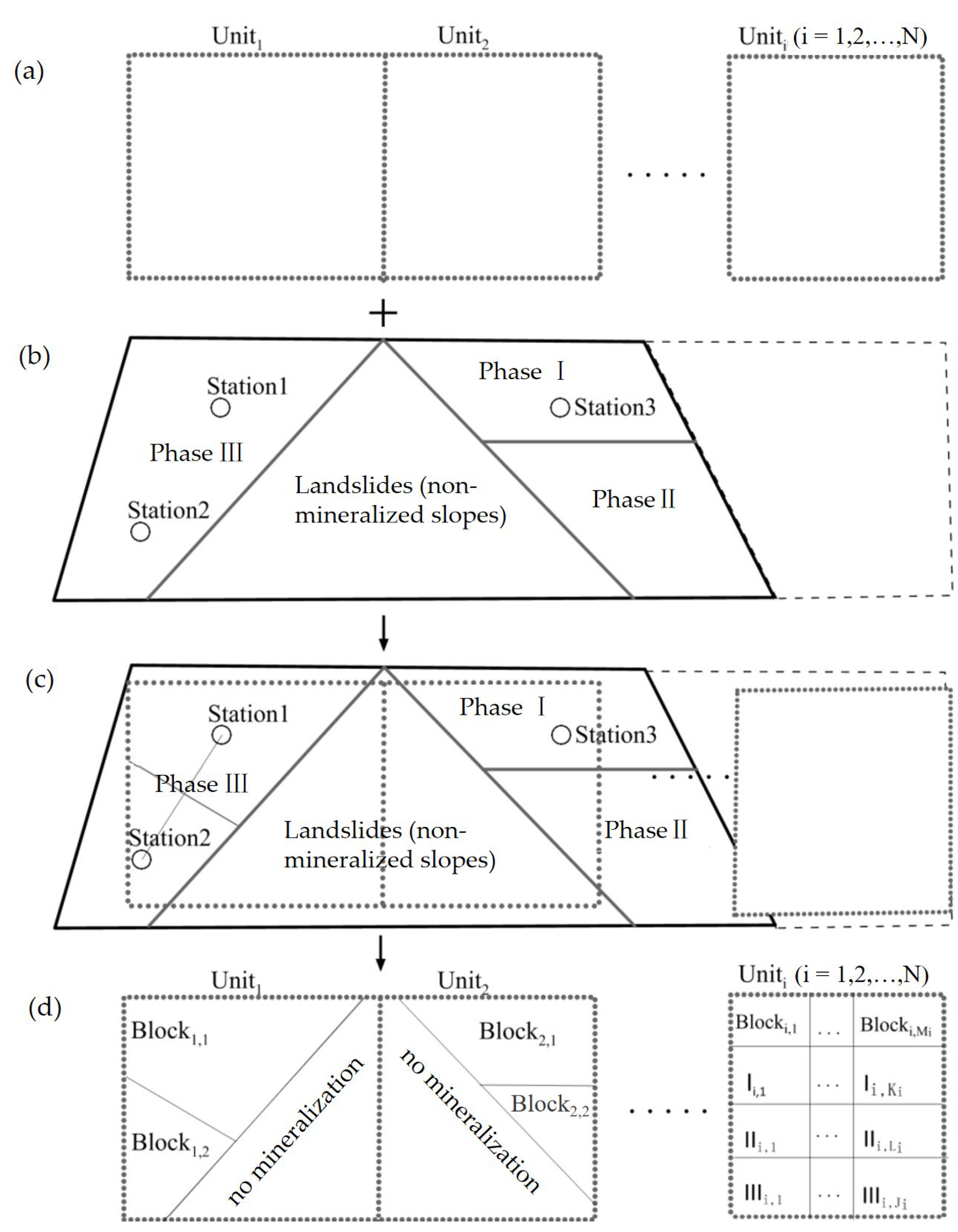
Slope landform type and water depth affect the distribution of cobalt-rich crusts. Generally, gentle slopes are covered by loose sediments without cobalt-rich crusts, while steep slopes are usually covered by cobalt-rich crusts. It should be indicated that steep slopes may have experienced landslides without cobalt-rich crust coverage. The thickness, coverage, and grade of cobalt-rich crusts also vary with water depth. Consequently, the adjacent areas with a similar distribution of cobalt-rich crust resources can be classified according to water depth and topography. Moreover, the boundary of the ore body can be divided according to the water depth classification. Based on the performed slope classification, types of seamount slope landforms can be distinguished and seamount slope micro-landforms can be divided. Furthermore, the mineralization period of the seamount can be summarized and identified. These different geomorphic types or mineralized slopes of different periods are geostatistical units, denoted as Block_i (i = 1, 2,…, N). In order to explore the original distribution pattern of crust thickness, an unsupervised classification method is used for topographic classification, and the third-order difference method is adopted in the slope calculation.

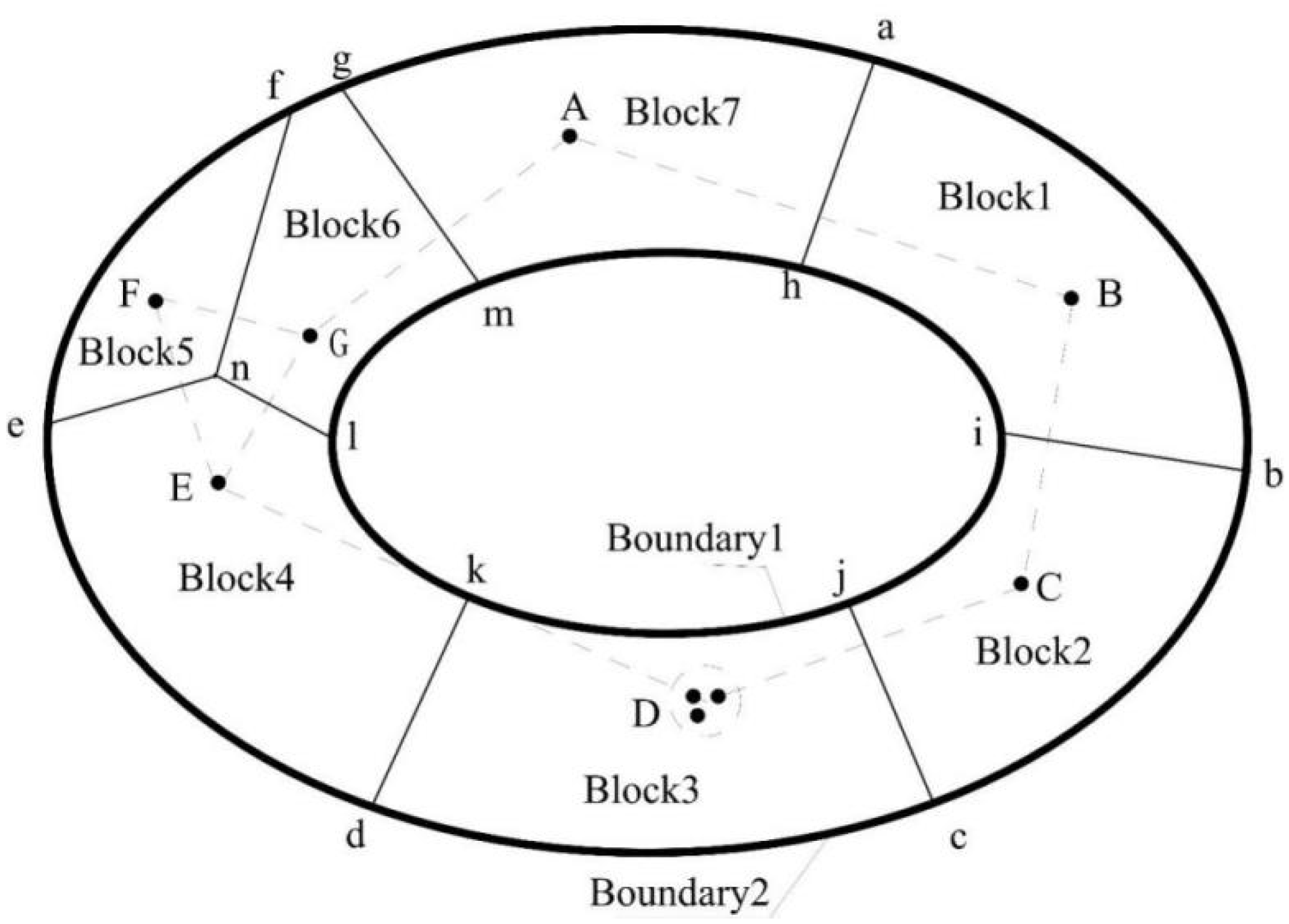
3.1.2. Adjacent Area Method

The main objective of the adjacent area method is to divide the geostatistical unit of the whole research target area by dividing polygonal blocks, while the sampling points are at the center surrounded by a block. These polygons are set together to form the whole mining area, and the mineral parameters of each sampling point are regarded as the mineral parameters of the corresponding polygon block [25].

At the first step, several geological stations with very similar spaces are combined into a single station. For example, station D is the combination of three geological sampling points. In the second stage, the normal line is drawn by connecting two adjacent points of the geological station. As an example, the vertical bisection ah of AB intersects Boundaries 1 and 2 at points a and h, respectively, and the vertical bisection of BC intersects Boundaries 1 and 2 at points b and I, respectively. Or some vertical bisector nodes cross each other, like n. These nodes delineate the area adjacent to the corresponding geological station with the geological station as the center. For example, abih and lnfgm delineate the areas adjacent to stations B and G, respectively. Finally, Blocks 1, 2,… and 7 delineate the remaining geological units. These blocks are the adjacent blocks of geological stations. This geological unit is automatically assigned to the geological characteristics and mineral parameters of the contained geological sites, or the mean value of multiple geological sites. As shown in Figure 3.

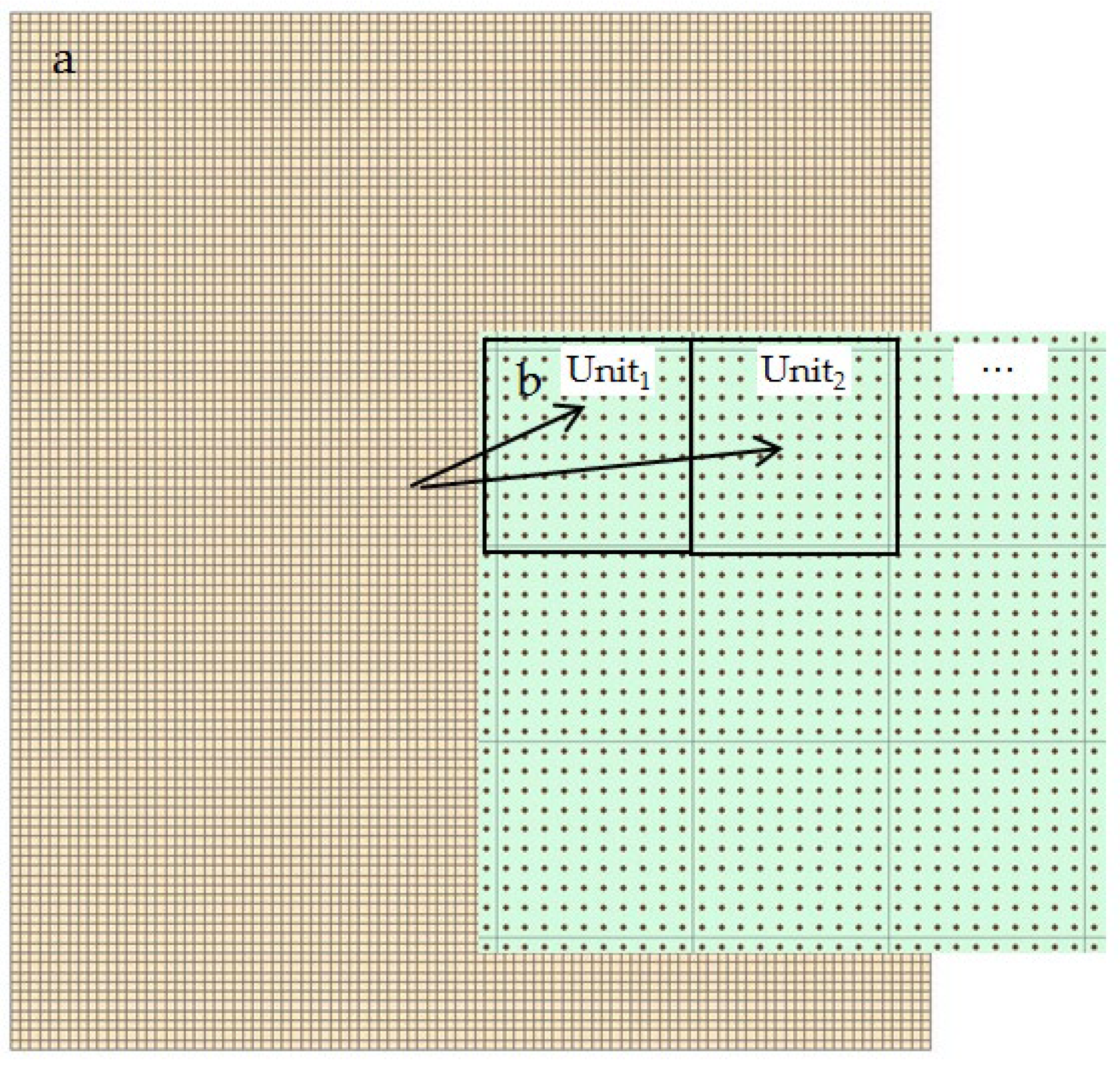
3.1.3. Grid Method

The grid size of units is determined according to the accuracy of the data obtained in the evaluation area and the requirements of the evaluation accuracy, so as to ensure that the statistical results of grid units meet the evaluation accuracy requirements of the region in a specific stage, to ensure that the number of points contained in each grid meets the statistical requirements, and to ensure that the calculation has statistical significance. Figure 4 shows that the evaluation area is divided into 1 km grid units, and each grid contains 10 × 10 information points. Regional grid units are divided according to the target accuracy.

3.2. Geostatistical Unit Assignment

For each statistical unit Uniti (i = 1, 2,…, N), the value of the resource parameter is the premise of estimating the resource quantity of the statistical unit. It is reminded that crust thickness is the most important parameter in the evaluation of cobalt-rich crust resources.

3.2.1. Station Proximity Area Assignment Method

According to the geological survey station, either the Thiessen polygon method or the buffer method is used to divide the mineralization block. Then appropriate values are assigned to the geostatistical units based on the station data.

After this, each statistical unit is subdivided into several mineralization blocks according to the slope mineralization partition and the geological station position control range. For example, an arbitrary statistical Unit_i (i = 1, 2…, N) can be divided into M mineralized blocks Block_i (i = 1,…, M), and K stage-I mineralized blocks I_i (i = 1, 2,…, K), L stage-II mineralized block II_i (i= 1, 2,…, L), or J stage-III mineralized block III_i (i = 1, 2,…, J). These blocks are controlled either by geological survey stations or by mineralization stages. Accordingly, the statistical unit can be divided into several mineralized blocks, in which each mineralized block is endowed with cobalt-rich crust resource parameters and mineralization characteristics according to geological station location or slope mineralization stage. To simplify, all blocks can be represented by Block_i (i = 1,…, N).

Statistical unit layers and mineral resource layers such as geological stations and slope mineralization zones are studied by spatial overlay analysis. The statistical unit is divided into several mineralized blocks, and the resource parameters and mineralization eigenvalues of these blocks are assigned by the geological station and slope mineralization characteristics, respectively. The resource reserves of each sub-block of the statistical unit are calculated separately and summed to obtain the resource reserves of the statistical unit. However, due to data sparsity, each statistical unit contains only one sub-block, and there may even be multiple statistical units in a single sub-block.

3.2.2. Spatial Interpolation-Assignment

In the spatial interpolation method, the geological station thickness is taken as the data point. Then spatial interpolations are carried out on each statistical unit to obtain the unique cobalt-rich crust thickness parameter. In the study area in the Il’ichev seamount, the reciprocal weighted average of distance, the moving window average, and the geostatistical method can be used as the spatial interpolation method. Since the conventional geostatistical method is not applicable to the interpolation application of seamount spatial data, Du et al. [24] proposed the geostatistical method for seamounts. To this end, the “slope–distance” variation function Kriging method was used to estimate the crust thickness of the mount. Then the distribution function is applied to statistically obtain the autocorrelations in the crust spatial distribution using adjacent information points with similar distribution characteristics. The Kriging estimation of the crust thickness can use only this function and the information points in this area to solve the Kriging equation and achieve interpolation. It shows that geological station information is the most effective way to improve the understanding of crust thickness distribution. Statistical methods can only use the existing conditions to approximate the spatial distribution of objects, and the approximation degree depends on the layout and density of sampling stations. After conducting a crust-thickness assessment based on geological station information and the “slope–distance” Kriging method, each statistical unit Unit_i (i = 1, 2,…, N) is assigned to achieve a unique solution for the cobalt-rich crust thickness in the statistical unit.

3.2.3. Expectation Value Assignment Method for Mineralized Block Segments

In order to explore the geology of the seamount, the survey data of several cobalt-rich crust stations were obtained, and the crust thickness was estimated by calculating the mean value of the station crust resource parameters in the geological unit. Then the expected value is used to assign a value to each statistical unit. This method is called the “expected value assignment method”. Although this method is simple and is an appropriate scheme to obtain the parameters of cobalt-rich crust resources with little spatial variation, it is not applicable to parameters with great spatial variation.

The main objective of the expected value estimation method is to count the resource parameters of all geological survey stations of at least one adjacent seamount and obtain the mean value of each parameter. Then the expected value of the whole seamount resources (hereinafter called “seamount expected value”) is estimated, and the expected value of the seamount is assigned to statistical units Unit_i (i = 1, 2,…, N). This is an ideal scheme to assign resource parameters of the whole seamount with a small deviation.

The expected value estimation of mineralized slopes over the same stage means that a seamount slope can be divided into several slopes with different mineralization stages. The expected value of resource parameters obtained from the resource parameters of the same mineralized slope station is called the same mineralization expected value. These values are assigned using blocks Block_i,j (i = 1,…, N; j = 1, 2,…, n) with the same expected mineralization value as statistical units. Compared with the whole seamount geological survey station, the slope station of the same mineralization stage has less resource parameter deviation, so it is an appropriate choice for the statistical unit assignment of the slope to the same mineralization stage.

This method can be implemented as follows: First, the mesh should be divided into a certain shape and size to generate N statistical layers. According to prior knowledge, survey data, and topographic features, seamount slopes were divided into non-mineralized and mineralized slopes in stages I, II, and III. Then the slope mineralization type zoning layer is generated accordingly. These mineralization zones have a certain control effect on the resource parameters of the cobalt-rich crust. For example, 2–3 layers of cobalt-rich crust thickness developed in the mineralization slope of stages I and II are generally larger than that of the single-layer mineralization slope of stage III. Cobalt-rich crusts with different mineralization stages have different densities and mineral contents. Consequently, the specific gravity, water content, and metal density of these layers are also different.

Figure 5 shows the method of assigning expectation values to mineralized block segments. Figure 5b shows the slope mineralization zones and geological survey stations: the left side is the stage III mineralized slope, in which there are two survey stations, No. 1 and No. 2; the upper right half is the stage I mineralized slope, in which the survey station No. 3 is distributed; the lower right part is the stage II mineralized slope, no survey site; the middle part is a landslide mass, a non-mineralized slope. Figure 5d shows the stage III mineralized slope is divided into two blocks by Thiessen polygon method according to two geological survey stations, and each block contains one survey station. For Unit₁, in addition to a non-mineralized block, has two blocks, Block_1,1 and Block_1,2, controlled by the geological survey station, both of which belong to the stage III mineralized slope. For Unit₂, in addition to a non-mineralized block, there are two blocks, one is the Block_2,1, controlled by the survey station No. 3, which belongs to the stage I mineralized slope. The other block, Block_2,2, without the control of the survey station, belongs to the stage II mineralized slope. Unit_i (i = 1, 2,…, N) represents any one of the N statistical units Unit_i.

3.2.4. Joint Assignment Method

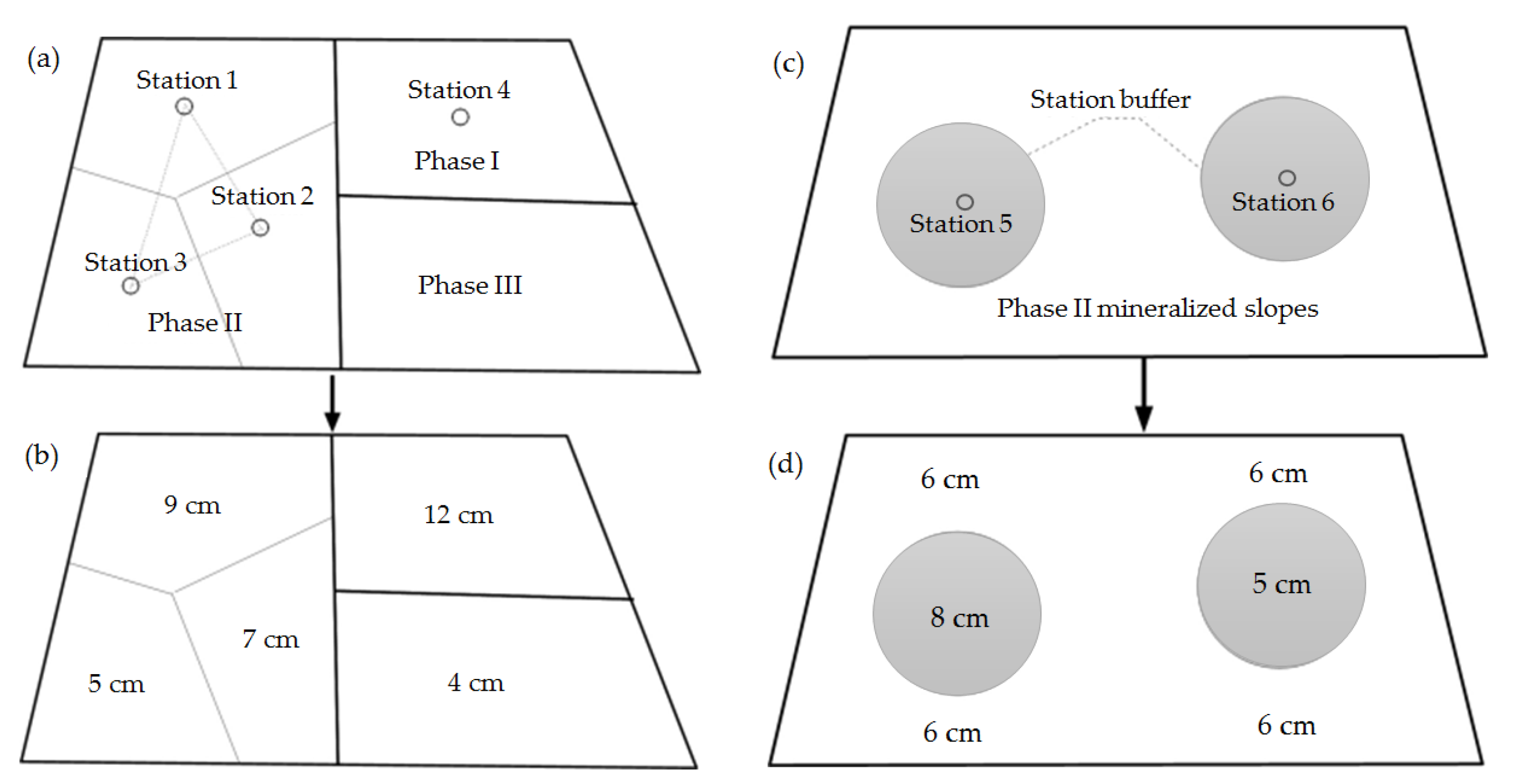
In the joint assignment method, it is intended to combine the foregoing methods to assign values. When there are many stations, the statistical unit of the slope is interpolated using the slope information points of the same mineralization stage. On the other hand, the Thiessen polygon method can be used to assign values in sparse stations. When there is no geological station control, the expected value of the slope of the mineralization stage is assigned. When the geological station is isolated, its buffer zone is used to assign values to the surrounding slopes, and other slope ranges are assigned to the expected values.

Figure 6 show that the cobalt-rich crust thickness of six geological survey stations Station 1,…, Station 6 are 9, 7, 5, 12, 8, and 5 cm, respectively. Meanwhile, the expected values of the cobalt-rich crust in mineralized slopes of stages I, II and III are 10, 6 and 4cm, respectively. Based on the joint assignment of multiple methods, cobalt-rich crust thickness values were assigned to the sloping block in Figure 6b,d, respectively.

4. Application

Studies show that the cobalt-rich crust thickness is affected by numerous factors, including slope type and water depth, and the spatial thickness distribution varies from 1 cm to 30 cm. Based on the accuracy required to evaluate the resource objectives, different assignment methods can be selected. (a) the adjacent area method, in which values are assigned to adjacent areas according to the crust thickness of the station; (b) the spatial interpolation assignment method, in which the crust thickness is assigned to statistical units (Thickness i, i = 1, 2,…, N); (c) the mineralized block assignment method, in which values are assigned to each block of the statistical unit (Thickness i,j, j = 1, 2,… Mi, i = 1, 2,…, N). Meanwhile, a composite assignment method can be used to obtain the crust thickness of statistical units.

4.1. Geological Grid Unit Division

In order to facilitate resource evaluation, geological grid units are divided first. The terrain data precision of the Il’ichev seamount is 230 × 230 m, which can be mapped into a 250 × 250 m grid. In order to ensure that each geological unit has sufficient statistical data, the study area is divided into 1 × 1 km grid units, in which each cell contains 25 statistical data points. The FishNet function of ArcGIS software was applied to perform the grid division of geological units. The CCD depth was considered as the 3500 m boundary to terrain an unsupervised classification model. This boundary is also the lower limit water depth of the sampling station and the crust growth coverage of the Il’ichev seamount is below 3500 m. Accordingly, the geological units of the study area were divided using 3706 geological unit grids. Figure 7 shows that the data points were distributed uniformly so that each unit contained 25 data points.

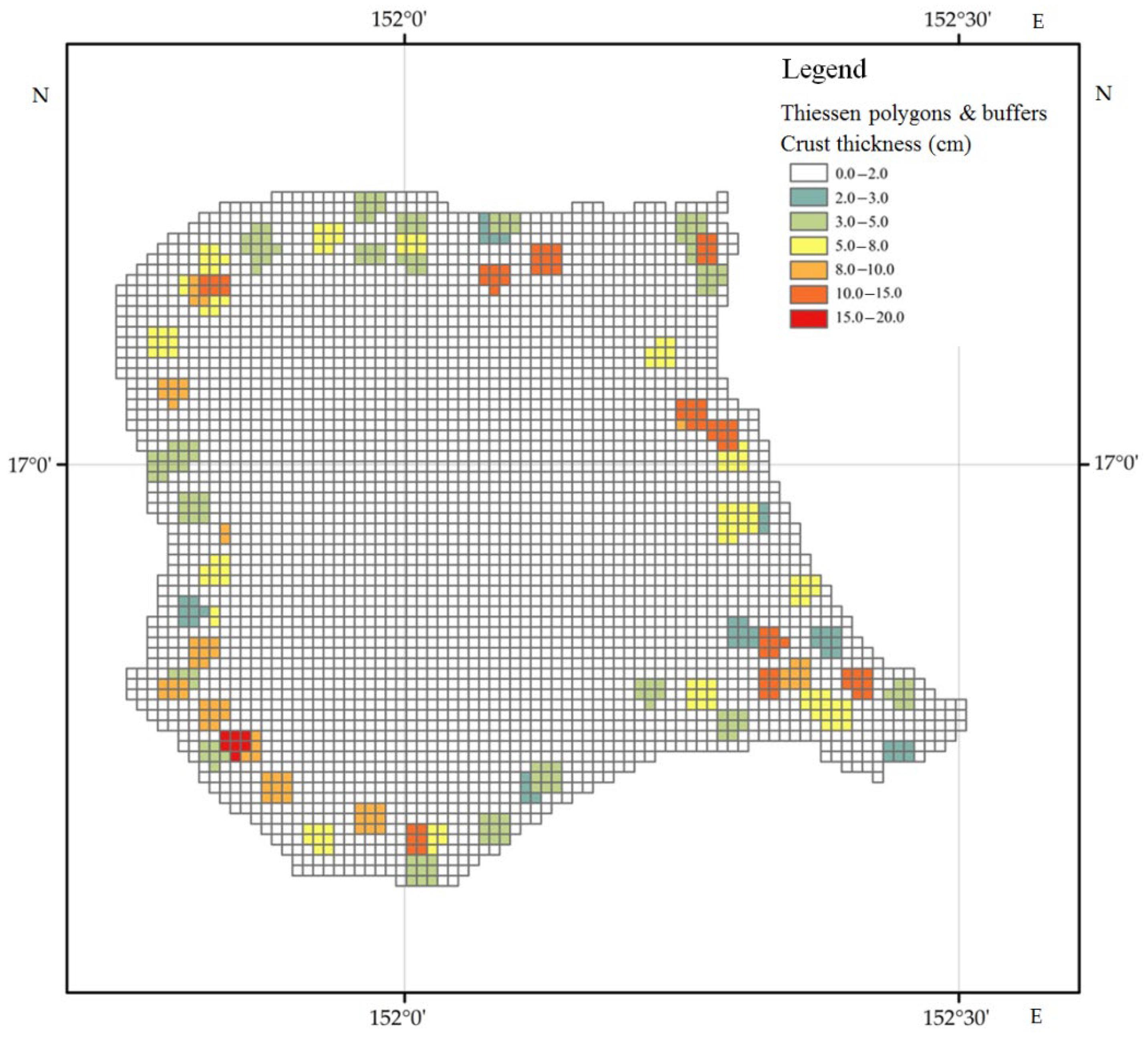
4.2. Adjacent Area Division and Statistical Unit Assignment

According to the geological sampling station, the influence area of the station was evaluated, the buffer radius was set to 1.5 km, the station buffer was established, and the preliminary block was divided as shown in Figure 8a. Taking the lower boundary of the ore body as the boundary, the Thiessen polygon method is used to generate the geological unit controlled by the station in the whole area and generate the blocks as shown in Figure 8b.

Information points of the Il’ichev seamount crust thickness are scarce. In order to make full use of geological sampling data, the crust thickness distribution parameters of the 1.5 km buffer were obtained according to the station shown in Figure 8a. Then the crust thickness parameters of the adjacent area were obtained using the Thiessen polygon shown in Figure 8b. The adjacent area controlled by the former station buffer is mainly used in the calculations, the boundary between adjacent stations delimited by the latter Thiessen polygon is supplemented, and the obtained value is assigned to the 1km grid unit. The assigned data are presented in Figure 9.

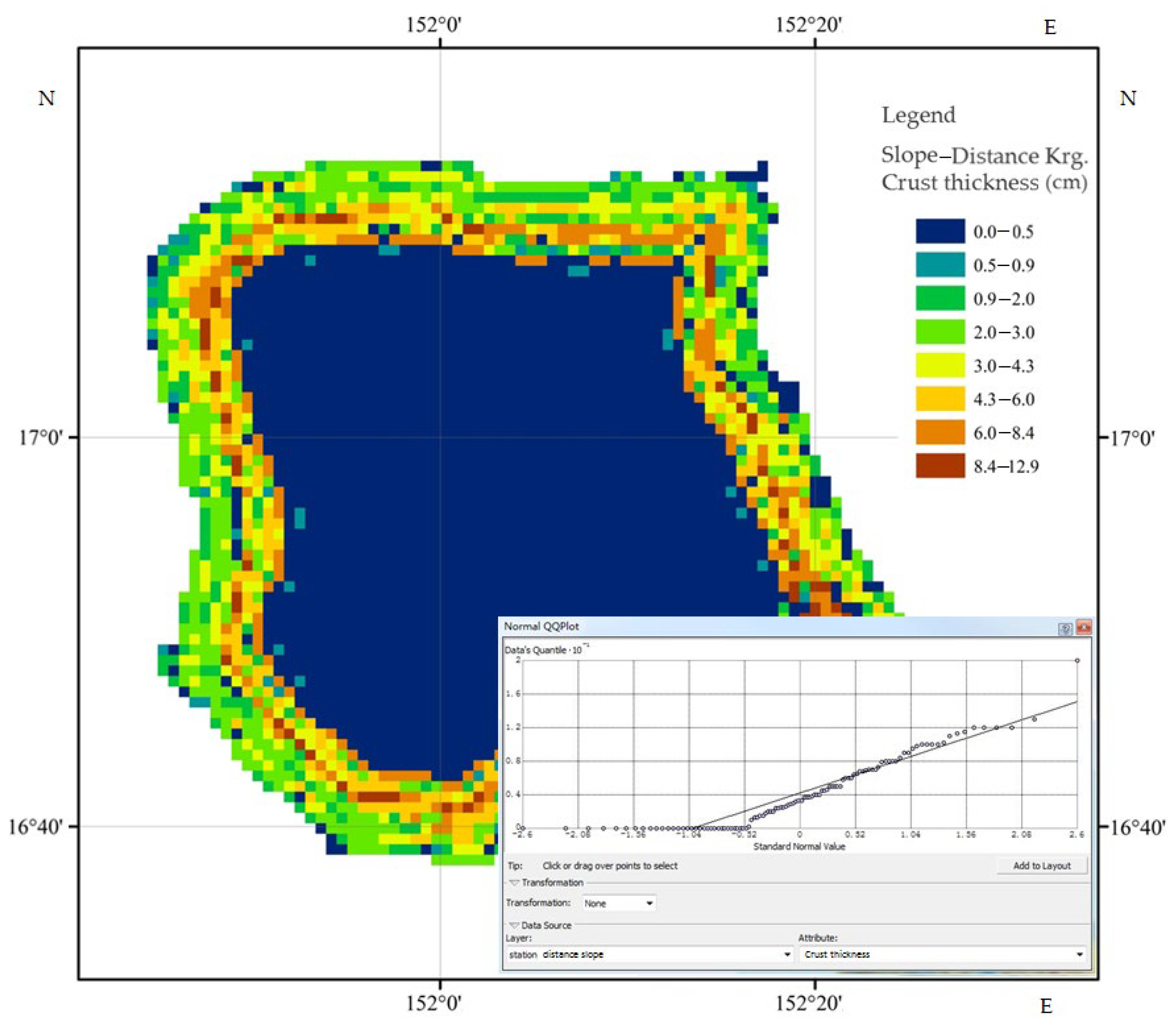
4.3. Spatial Interpolation-Assignment

In order to realize the Kriging interpolation method of “slope–distance”, the topographic data were processed to make its range consistent with the coverage range of the divided geological unit (1 × 1 km). Then the slope method is applied to calculate the slope of each point in the 250 m precision topographic data. Finally, the average slope of 25 points in each geological unit grid is calculated to obtain the slope of the geological unit. The crust survey station and geostatistical unit were spatially superimposed and correlated, and the average slope of each station was calculated. The isobathic distance of the 3500 m boundary to the lower boundary was calculated using the Near method in ArcMap. The calculated “distance” and “slope” are used as the coordinate values of the “slope–distance” coordinate system of the station points, and the spatial layer “slope–distance.shp” is regenerated for all the station points in ArcMap. The station site statistical analysis method in the new layer was used to simulate the distribution function of the crust-thickness data using the Kriging method in Geostatistical Analyst. The QQ histogram in Figure 10 shows that, except for the mountaintop part, the crust thickness of other stations follows a normal distribution. Based on the simulation results and the experience of crusting investigation, spatial interpolation with a radius of 2 km was carried out and the obtained results are presented in Figure 10. Accordingly, Figure 11 illustrates the superimposed assigned values of statistical units that have no assigned values after step 4.2.

4.4. Mineralized Block Phase Classification and Statistical Unit Assignment

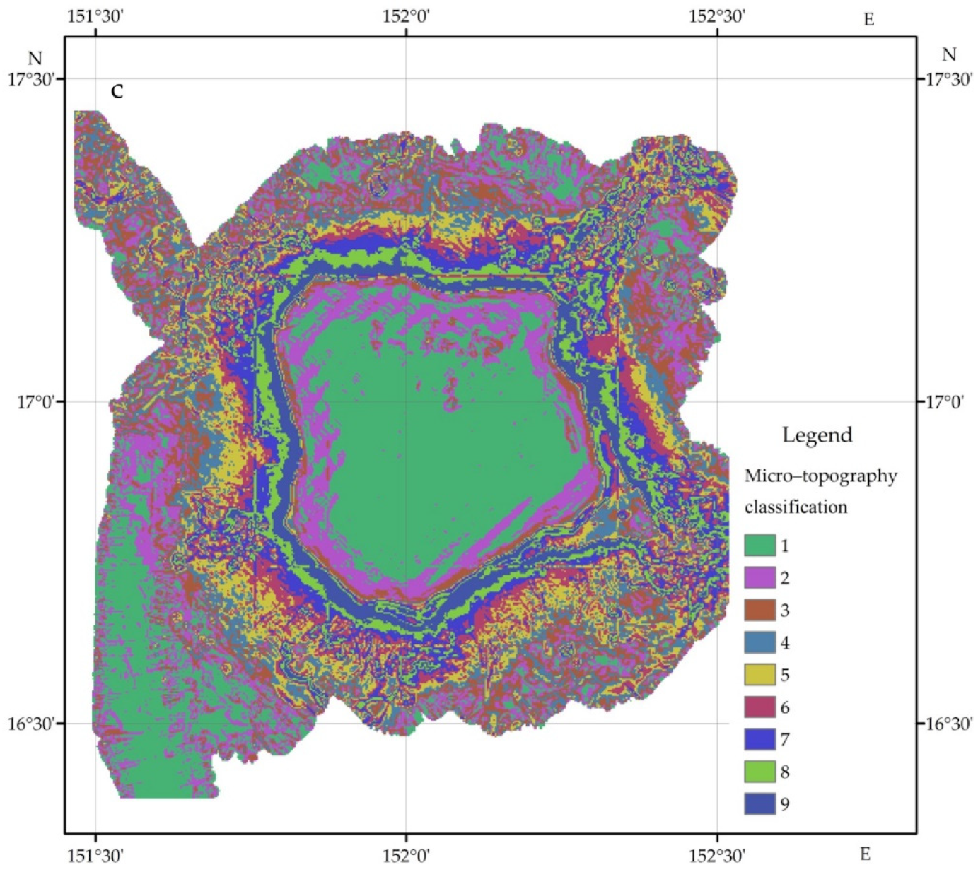
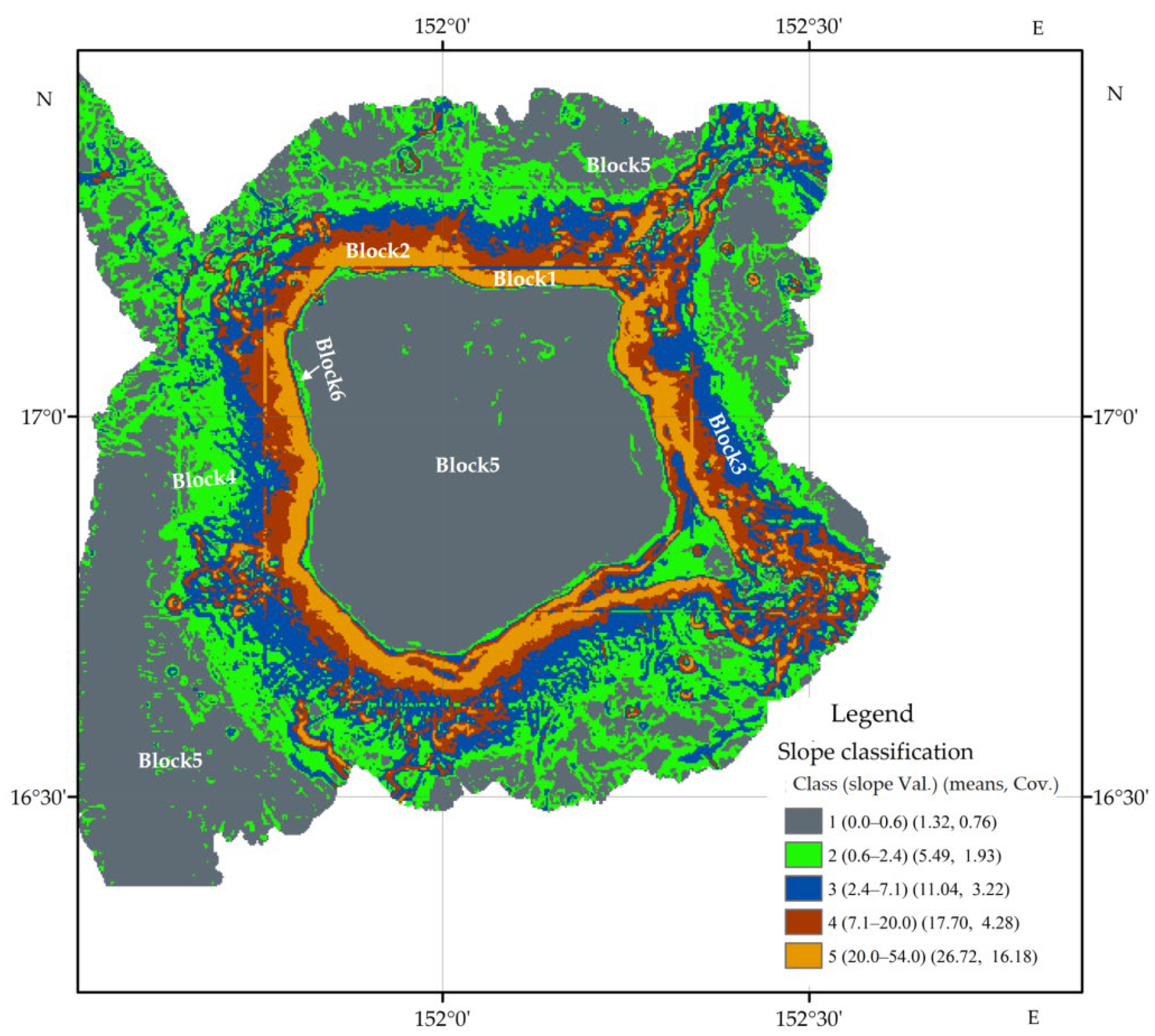
In the present study, the slope method is used to calculate the slope, and then the Iso-Cluster Unsupervised Classification method is used to perform unsupervised classification on slope data. According to the terrain variation, the boundaries of different terrain types are divided and vectorized, and the boundary covered by crust geological units (isotherm of 3500 m) is used to define the lower boundary. Figure 12 shows that the boundary values of slope unsupervised classification were 0.6, 2.4, 7.1, and 20.0. The mean slope of each class is 1.32, 5.49, 11.04, 17.70, and 26.72, respectively. The covariance of each classification gradually increases. According to the topography slope classification results, the whole seamount is divided into geological blocks: Block1, Block2,…, Blockn. As shown in Figure 12.

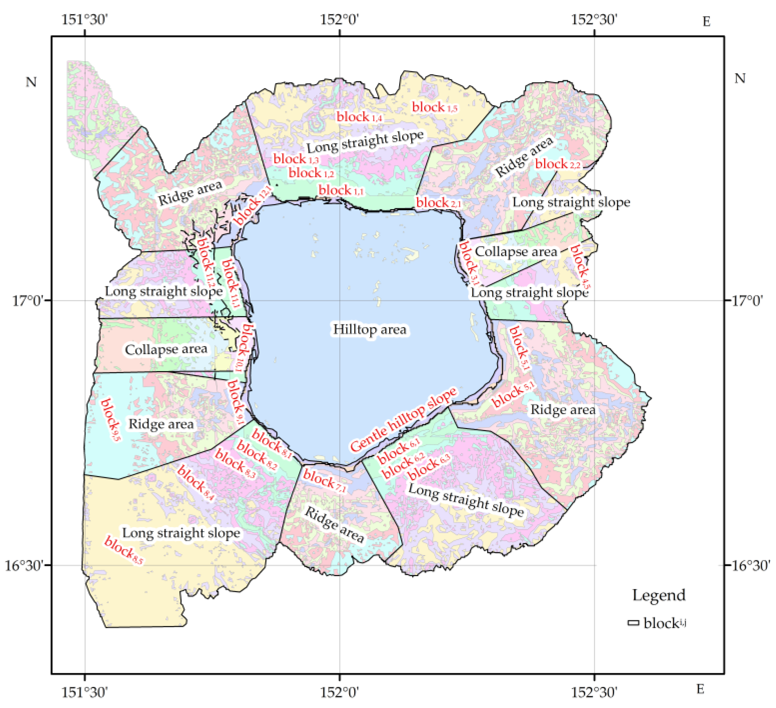
Combining the micro-terrain classification results with the original topographic features and the visual morphology of slope changes, the topography of the Il’ichev seamount can be divided into gentle hilltop area, gentle hilltop slope area at the junction of the hilltop and slope, ridge area where various micro-landforms are concentrated, long straight slope area, and “spoon-shaped” collapse area. These areas are presented in Figure 13. The collapse area is a landslide in geological history. The crust thickness on the exposed bedrock is 0, and the slope is generally greater than 15°. However, a slope greater than 15° is not conducive to the terrain mining techniques and should be excluded from the encircled ore area. In this regard, the proportion of unfavorable terrain in each exploration unit should be estimated.

Slopes covered by cobalt-rich crusts are known as mineralized seamounts or mineralized slopes. This kind of slope has two features: it is not a gentle slope, and no slope reconstruction has occurred since the middle and late Quaternary periods. The distribution of the resource amount on the mineralized slope is a naturally occurring amount. In terms of topography and landform, it is manifested as a “gentle hilltop slope”, “long straight slope”, or relatively stable “ridge area”. Slopes that are not covered by sediments and are suitable for mining are considered favorable slope areas. The proportion of these slope areas to the entire area in grid cells is an important parameter to estimate recoverable ore or metal reserves. According to the topographic and geomorphic classification results, the whole seamount is divided into geological blocks: Block1, Block2,…, Blockn. As shown in Figure 13.

According to the results of the above two steps, the blocks divided from topography slope classification and landform classification are superimposed to create more detailed geological blocks: Block_i,j (i = 1, 2,…, N; j = 1, 2,…, n), as shown in Figure 14.

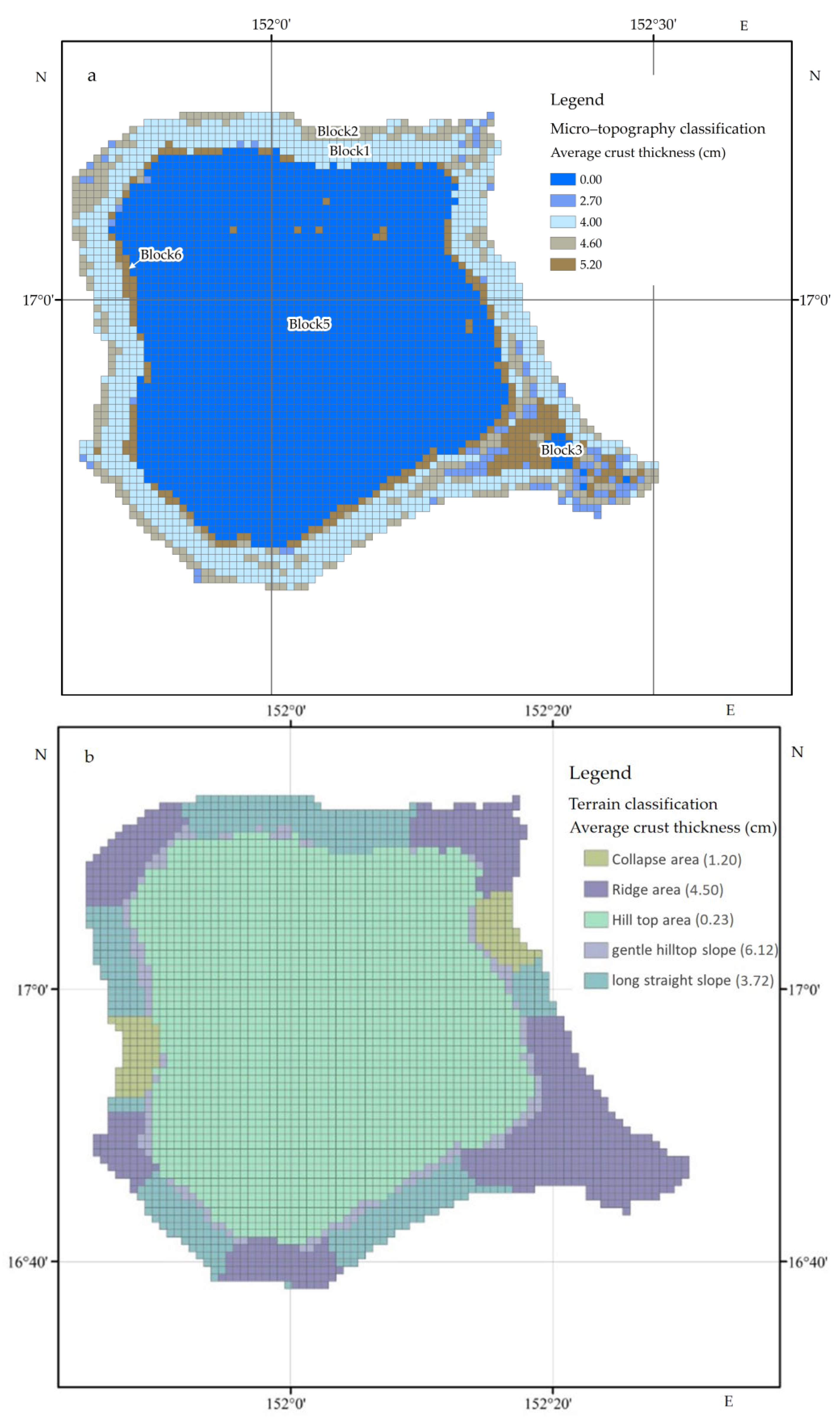
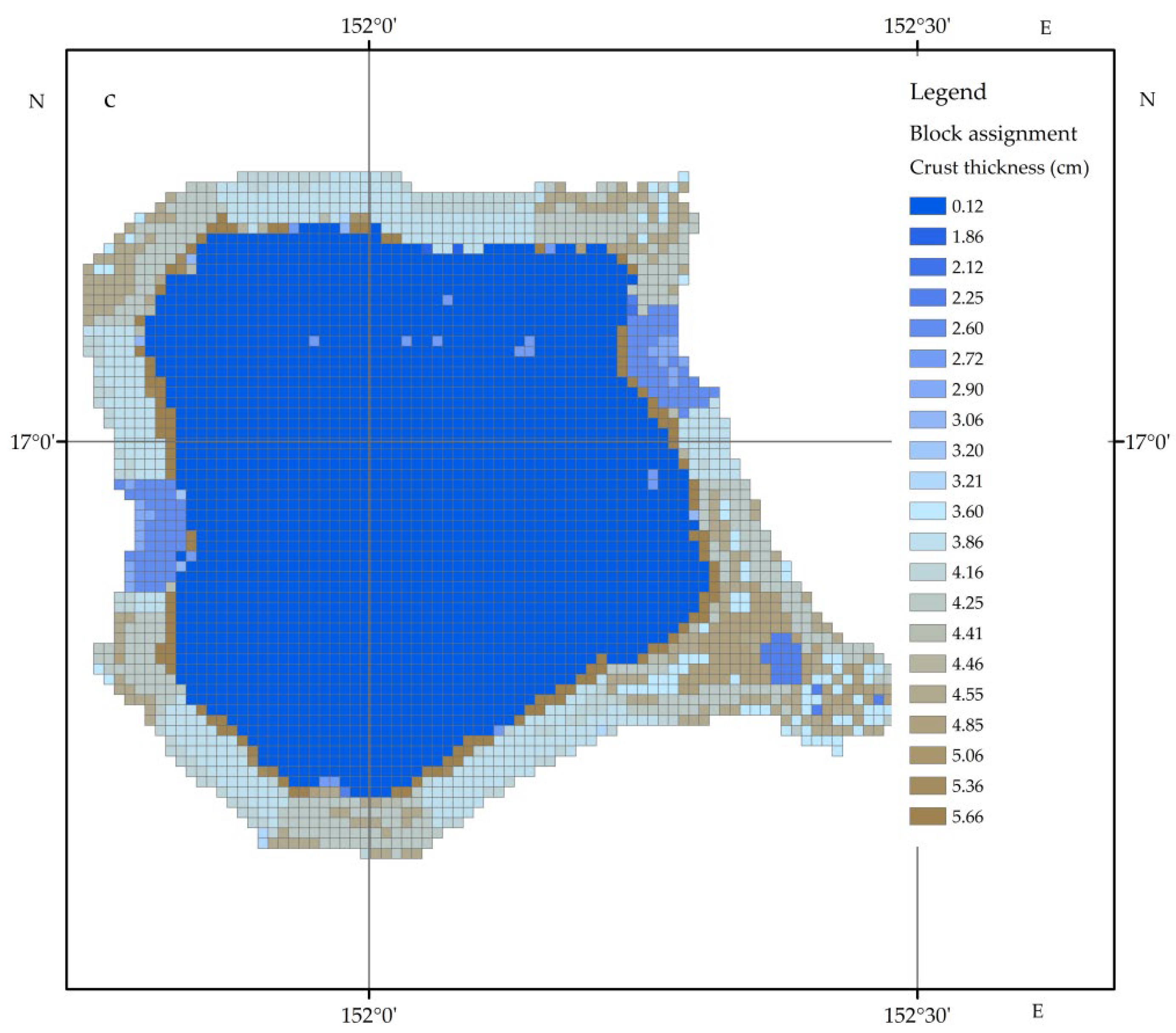
In Figure 12, the mean thickness of the crust stations of block1, 2, 3, 5 and 6 are 4.00, 4.60, 2.70, 0.00, 5.20, respectively, as shown in Figure 15a. And the block4 originally in Figure 12 is not involved in this figure. In Figure 13, the mean thicknesses of the crust stations in the five geomorphologies are 1.20, 6.12, 4.50, 3.72, and 0.23, respectively, as shown in Figure 15b. Then the crust thickness of the geostatistical grid cell was obtained by superposition of Figure 15a,b, as shown in Figure 15c. The Figure 15c shows the obtained crust thickness assignment results from the classification of topography slope and geomorphological classification.

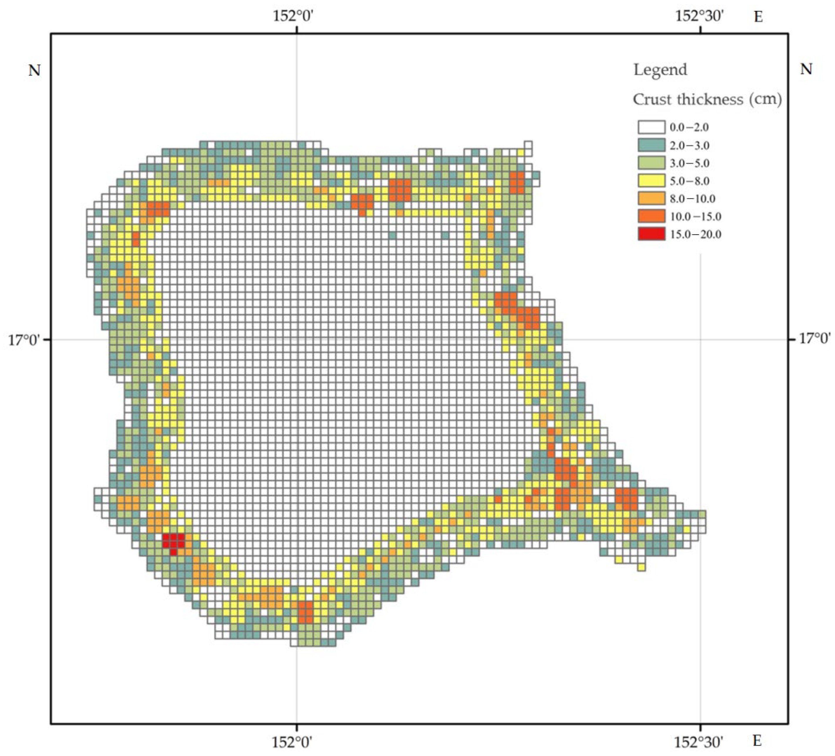
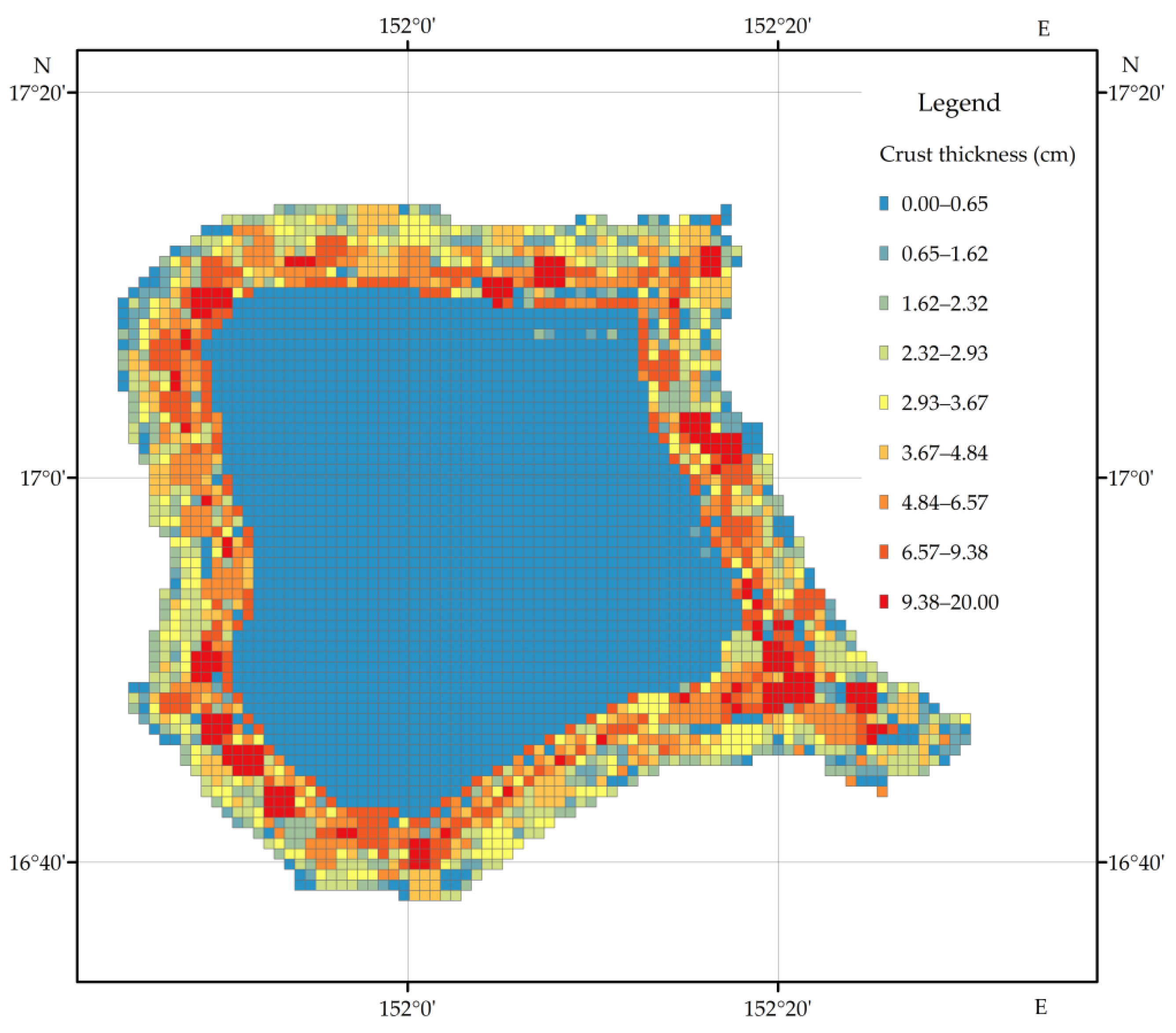
The obtained grid unit assignment results are combined to supplement the crust thickness of the unassigned grid unit, thereby assigning the entire regional geological unit. The final grid unit assignment is shown in Figure 16.

Figure 16 indicates that the crust thickness aggregates near the survey station. This may be attributed to the assignment method. As the topography of the seamount changes, it is characterized by a ring-shaped distribution, and the thickness distributions in the collapse area and the long straight slope areas with a large area, are obviously different from the other parts. The obtained results are consistent with experimental data [24] and previous investigations [10].

5. Discussion

Cobalt is a strategic material so cobalt-rich crust resources in seamounts have attracted many scholars worldwide [26,27]. Accordingly, exploring cobalt-rich crust resources is of great significance. Crust thickness is the most important parameter in estimating cobalt-rich crust resources. Currently, there is no general and effective method to estimate cobalt resources. Aiming at resolving this shortcoming, a fine topographic survey was carried out to evaluate the parameters of crust thickness using geostatistical unit division and assignment methods.

The geological unit division is very important in the evaluation of cobalt-rich crust resources. The geostatistical unit division and crust thickness assignment methods involved in this paper are summarized by combining the basic theoretical research of previous scholars with current technical methods. The “adjacent area–”slope–distance” Kriging interpolation–geological block“ method is the more suitable and comprehensive partition and assignment calculation method under the current situation. Its effect is better than single assignment methods.

Considering technical limitations, geological station sampling data are the most accurate data on seamount crust parameters that can be obtained at present. In the present study, the geological cells were divided based on the neighborhood area method. In order to ensure the performance of sampling stations and to effectively utilize data, station buffers and Thiessen polygons are assigned to the geostatistical grid cells.

Combined with the Il’ichev seamount’s topography and the crust sampling station, slope reconstruction activities such as landslides and collapses have occurred on the flanks of the seamount slopes since the middle and late Quaternary. These interactions removed various sediments including cobalt-rich crusts on the surface of the landslide bodies and buried them. Accordingly, such slopes are also called “reconstructed seamount slopes”. Since the late Cretaceous, seamounts reconstitution may have occurred several times. Subsequently, cobalt-rich crusts with the most complete crust (layers R, I, II, III) were developed in the mineralized slope without reconstructing movement. Mineralized slopes that have not undergone slope reconstruction since the early Tertiary period generally have three layers of crusts, including layers I, II and III. Since the Miocene, layers II and III developed on slopes that had not undergone slope reconstruction. Since the Pliocene, only layer III developed on slopes that had not undergone slope reconstruction. In this article, a novel method is proposed to classify the mineralization periods of seamounts using topography and geomorphology combined with geological theory, a priori knowledge, and survey data. The geological units and geostatistical grid cells can be divided according to mineralization periods, and the mathematical expectation method can be applied to assign the crust thickness values to the geological units and geostatistical grid cells from the mineralization perspective.

Figure 14 indicates that mineralized slopes at different stages can be identified by the classification and identification of slope topography and geological sampling control of key stations. Cobalt-rich crust slopes with R, I, II, III and I, II, III layers are collectively referred to as stage I mineralization slopes; the cobalt-rich crust slopes of layers II and III are called stage II mineralization slopes; the cobalt-rich crust slopes of layer III are called stage III mineralization slopes. Mineralization slopes of different stages are regarded as different geological units. Compared with the whole seamount geological survey station, the slope station of the same mineralization stage has fewer resource parameters, which is more suitable for the statistical unit assignment of the slope of the same mineralization stage. The partition method is based on ArcGIS technology, which makes the later applications operable.

There are a few investigations on the resource assessment of seamounts. These studies are mainly focused on conceptual and methodological descriptions [18,19,20], and resource assessment at larger scales [12]. In this article, compared with previous assessments using a particular method alone, the results of the crust thickness assessment on the Il’ichev seamount were obtained using an integrated approach with more details. To this end, the geostatistical unit was divided using the adjacent area method based on the station buffer and the Thiessen polygons method. Then the important position of information obtained from station sampling is firmly established. Then the "slope–distance" method is used for interpolation. The obtained crust thickness distribution ranged from 0–12.9 cm, which is consistent with the published results [1]; the “Ring” distribution characteristics due to water depth, topography, and distance from the ore body boundary can be observed clearly. Then the remaining geostatistical grid cells were assigned based on the mineralization period and the mathematical expectation method. The obtained results of the integrated assessment significantly outperform the previous single-method assessments: the results of the integrated method retain the influence of the station itself; extend the influence range of the station by interpolating; and compensate for the shortcomings in the evaluation by sampling points from a metallogenic point of view.

In the application of the spatial interpolation assignment, the “slope–distance” Kriging method [24] was implemented and values were assigned to grid units. Moreover, the data processing and analyses were realized by ArcGIS, and the relevant implementation methods were introduced.

6. Conclusions

Compared with previous research methods, a detailed analysis was carried out on geological sampling data and fine topographic data of the Il’ichev seamount. Then the mineralization stages and the geological units were divided according to the performed analyses. Meanwhile, the crust thickness evaluation was formulated by several methods including the station buffer, the adjacent area method, the expected value of the crust thickness of the geological block, and the spatial interpolation statistics. Firstly, the adjacent area method was used to calculate the crust thickness in the buffer area of 1.5 km area around the station. Then, the crust thickness covering the whole mineralized area was estimated using the Thiessen polygon method. The optimal crust thickness within 1.5 km was obtained by combining the two methods and the thickness value is assigned to the crust evaluation grid unit. Secondly, the topographic data, which are finer than the station, were used in the estimation and the “slope–distance” Kriging interpolation method was applied to calculate the crust thickness in the mineralization area. Meanwhile, the crust thickness in the optimal effective radius area is used to compensate for the gap in the previous grid element estimation results. Finally, the mathematical expectation method based on the topographic classification was used to calculate the average crust thickness of the remaining grid units. The performed analyses revealed that the proposed “adjacent area–”slope–distance” Kriging interpolation–geological block” method has promising performance in the evaluation of the Il’ichev seamount’s crust thickness. This method can be used to achieve more certain and detailed results. In order to ensure that the crust thickness in the area adjacent to the stations is closer to the crust thickness in the neighboring known stations, the spatial influence of the sampling stations is determined first. The “distance–slope” method is based on station sampling data and bathymetric topographic data. This method can be applied to achieve a more detailed crust thickness assessment and ensure that the estimated data affected by the sampling point are consistent with the measured data. The mathematical expectation method of crust thickness estimation based on the subdivision of seamount mineralization stages can be applied to compensate for large deviations originating from the lack of data points. Consequently, the crust thickness can be estimated in the area with insufficient information points from the perspective of the mineralization mechanism. This article provides a simple and effective implementation of the full method process based on ArcGIS, which outperforms the conventional methods in evaluating the seamount crust thickness, without comprehensive investigations.